Intangible Assets – Influence on the “Return On Equity” (S&P100 Index)

15-16 November 2018

Seville Spain

ISBN: 978-0-9998551-1-9

Vision 2020: Sustainable Economic Development and Application of Innovation Management

from Regional expansion to Global Growth

Editor

Khalid S. Soliman

International Business Information Management Association (IBIMA)

Intangible Assets – Influence on the “Return On Equity”

(S&P100 Index)

Alcina NUNES

Unidade de Investigação em Gestão Aplicada (UNIAG), Instituto Politécnico de Bragança (IPB), Bragança, Portugal, alcina@ipb.pt

Jair GARCIA

Instituto Politécnico de Bragança(IPB), Bragança, Portugal, garcia.gar_cia@hotmail.com

José LOPES

Centro de Investigação em Contabilidade e Fiscalidade (CICF), Instituto Politécnico de Bragança (IPB), Bragança, Portugal, jlopes@ipb.pt

Vladimir ZEFIROV

Peter the Great St. Petersburg Polytechnic University, St. Petersburg, Russia, v.zefirov@mail.ru

Abstract

In the 21st century, the most valuable strategic resources for business enterprises will no longer be physical assets such as land and machines, but rather intangible assets (IA) such as knowledge, patents, and intellectual property rights. This study aims to analyze the effect of IA (exclusively those that are recognized and shown in the balance sheet) on the return on equity (ROE). In order to analyze the influence of IA on ROE, the study used components of the Standard and Poor 100 Index (S&P100). Due to some research restrictions, 68 companies were selected as the study’s sample. The research results were obtained using the Ordinary Least Square (OLS) method. According to our findings, the influence of IA on ROE is approximately 34% excluding goodwill and 31% including goodwill.

Keywords

Introduction

Nowadays, companies are acquiring and develop more non-physical assets. Therefore, a question arises – what is the effect of the intangible assets in companies’ performance? A study performed by Aboody and Lev (2000) shows that companies who had intense research and development programs (R&D) obtained higher gains than those without them. Considering the relevance of the issue, this research aims to study the influence of the Intangible Assets (IA) - exclusively those that are recognized and showed in the balance sheet - on the Return on Equity (ROE). Due to the accounting segregation of the IA and the goodwill, the analysis considers both IA and “IA including goodwill”. Therefore, the main research question can be stated as follows: what is the influence of IA (recognized in the balance sheet) on companies’ performance, and, in particular, on the return on equity? In order to answer the question, two operational objectives were established: (i) analyze the impact of IA on ROE and (ii) analyze the impact of IA, including goodwill, on ROE. The sample of the study is based on a group of companies that are components of Standard and Poor 100 Index (S&P100). The S&P100 index comprises 101 companies across multiple industry groups; however, due to the requirements established for this project, only 68 companies were selected as the study’s sample. The Three-Step Dupont Model, which lies in a broken form of Return on Equity (ROE) original formula, is used as a starting point. The model comprises the

three following factors: net profit margin, asset turnover and equity multiplier. For the study purposes, the equity multiplier was modified to isolate the intangible assets, obtaining a modified version of the Dupont model. Next, the Ordinary Least Square (OLS) was used to analyze the impact of the intangible assets over the return on equity.

Intangible Assets And Return On Equity – Brief Literature Review

Intangible Assets

Intangibles gained more importance in firms’ accountancy at the end of the past century. Further, IA is a fundamental factor of value (Cañibano, Garcia-Ayuso and Sánchez, 2000). International Accounting Standard (IAS) and International Forms of Reporting Standards (IFRS) have made major advances in defining and recognizing IA on financial statements. Although, today’s accounting framework is distant to comprehend all intangibles resources. The term IA was first introduced in the mid-80’s (Artsberg and Mehtiyeva, 2010; Bryan, Rafferty and Wigan, 2017). Until the year 1997, the International Accounting Standards Board (IASB) issued the IAS No. 38. IA are contained in “other assets” section, that consist of permanent investments and the IA (Guerard and Schwartz, 2007), at the bottom of the assets section in the Balance Sheet financial statement. The Financial Accounting Standards Board (FASB) framework defines assets as the possible future economic benefits obtained as a result of past transactions and IA as an identifiable non-monetary asset without physical substance. This standard outlines the recognition, valuation and disclosure of IA on financial statements. Additionally, the IAS 38 provides the scope where the IA is to be found. The issue of this standard was in response to the demand of an international demand on recognizing intangible resources. This demand came along with the surge of the Knowledge-based Economy (KE) The IA gained more importance after the surge of the KE. Aligned with the globalized economy, this microeconomic model is focused on intangible resources such as expertise, patents, data and information (Carrillo, 2015; Bratianu, 2017).

This economy framework is stimulating firms to drive their business from massive production processes to fostering knowledge that produces innovative and cutting-edge products. Furthermore, this framework promotes a change in businesses’ sources of value pivoting to intangibles (Pucci, Simoni and Zanni, 2015). KE is habitually associated with technological, media, financial and medical industries. Nevertheless, this economic model affects all industries. The influence of this model can be seen by in the rise of IA, which has almost doubled in the last 16 years, from $19.8 trillion to $47.6 trillion, see Figure 1. Most of the high-tech and pharmaceutical companies in 2005 had more than 90% of their assets in intangibles (Bryan, Rafferty and Wigan, 2017).

One of today’s problems regarding IA is the disclosure of some intangibles. Scholars, professionals and audit firms have been discussing the need for a modern form of reporting of IA due to the improper recognition and valuation of some IA (Niculita, Popa and Caloian, 2012; Pucci, Simoni and Zanni, 2015; Bryan, Rafferty and Wigan, 2017; Tahat, Ahmed and Alhadab, 2017). Within the current accounting standards, most of the intangibles are not recognized, leaving many intangibles unacknowledged.

The study conducted by Heiens et al., (2007) regarding the implication of the IA on firms’ holding returns suggests that IA other than goodwill have a significant positive impact, in contrast, high accumulation of goodwill and R&D expenditures have a negative impact on shareholders’ returns. Heinens’ study proceeds using the resource-base view, the mentioned study obtained data from 1.675 companies recorded by the Center for Research in Security Prices in 2001. The results support the premise for a positive relationship between the IA and shareholders’ returns, specifically those intangibles that are used for advertising have a slight impact on long-term returns.

Tahat et al., (2017) studied the impact of intangibles on firms’ current and future financial and market performance within the companies constituting the United Kingdom’s Index FTSE 150 from 1995 to 2015. The study was focused on the role of goodwill and R&D on firms’ performance. The authors support the idea that financial statements are not revealing accurate present information regarding

financial performance. Moreover, the study emphasizes the need for studies targeting future performance. The proxies employed in earnings per share were a return on assets (ROA) and ROE. The findings display a positive impact of investments in intangibles on the company’s future performance, yet for the short term, the relationship goes in the opposite way. The results are consistent with market-based and resource-based theories, assuming IA is a relevant factor for sustainability of earnings and boost future performance. Additionally, the study though not significantly negative relationship between R&D and companies’ current market operation.

A universal definition of IA has not been established hitherto, however identifiable IA have much in common with tangible long-lived assets. Assets are recognized only if they will bring future benefit to the firm (Tahat, Ahmed and Alhadab, 2017), yet intangibles have the peculiar characteristic that besides providing future benefit, they are also recognized if they could prevent or block other competitors to enter in the market, e.g., patents, or licenses. The following characteristics must be present to qualify an item as an asset (Wittsiepe, 2008):

The asset must provide probable future economic benefits that enable it to provide future net cash inflows;

The entity is able to receive the benefit and restrict other entities’ access to that benefit; The event that provides the entity with the right to the benefit has occurred.

As it was said before, a more complex framework is used to define IA. One case study had to integrate the federal court, local real estate laws, international financial standards and industry literature about IA to provide not a definition but a scheme to identify intangibles as assets (Understanding Intangible Assets and Real Estate: A Guide for Real Property Valuation Professionals, 2016). This exercise produced a 4-step test that helps managers and assessors to recognize easily if an intangible is subject to be considered part of the assets.

Intangibles should be identifiable.

Intangibles should possess evidence of legal ownership.

Intangibles should be capable of being separate and divisible from the real estate. Intangibles should be able to be legally transferred.

These four qualifications in addition to the 3 previously mentioned must be present to determine an intangible as an asset. The IAS 38 (IFRS Foundation, 2014) defines an “intangible asset as an identifiable non-monetary asset without physical substance”. For the purposes of this study, IA is defined as all identifiable resources that lack the physical substance that could be self-generated or traded, and for those intangibles that were acquired by past trade transactions their usage could last for a limited or unlimited period and are shown in the balance sheet financial statement. It is necessary to mention that only those IA which are recognized in the financial statements were used in this study. Intangible resources provide a composition of knowledge, information, intellectual property, and experience. IA could be acquired as a result of market transactions or self-generated and they could have a definitive or indefinite life (Wittsiepe, 2008; El-Tawy and Tollington, 2013). Goodwill has a singular treatment. It is, indeed, an intangible asset; nonetheless, depending on how it was gained (Saunders and Brynjolfsson, 2016), it could be treated as part of business combinations (IAS 3 and FAS 141) or as any other IA. The reason that self-generated goodwill is not recognized is, in most of the cases, because it is still under development and cannot be separated (Artsberg and Mehtiyeva, 2010; Saunders and Brynjolfsson, 2016). A comprehensive scheme that resumes the classification of intangibles can be found in a study developed by Vilora, Nevado and Lopez (2009); the scheme resumes accurately the classification of intangible assets.

The literature reviewed of IA point towards IA as a strong component of a company’s financial potential. However, it should be pointed out that IA by themselves are not enough to maximize profit or

significantly increase ROE. IA must come along with tangible assets to develop continuous growth. Is also necessary to emphasize the need for proper classification and early recognition of IA.

Return on Equity

Many financial tools are available to measure companies’ financial performance. On the one hand, investors, managers and shareholders can perform a financial statement analysis to determine if a company is profitable or not. On the other hand, ratios are useful tools to measure the extent of profit earned by companies in a certain period of time (Jensen, 2008). Financial ratios were created to provide quick indicators regarding companies’ financial situation and to measure economic effectiveness. Most ratios use book values. This means that information is taken from companies’ financial statements. Some other ratios use market value for forecasting purposes and better decision making. Financial ratios that use market values provide more accurate information about companies in “real time”, compared to the historical information provided by financial statements. One of the most used and well-known profitability ratios is the return on shareholders’ equity (ROE). This ratio has been used to measure companies’ efficiency in profit generation, and due to the ratio uses the net income as a benchmark to measure profitability (Kijewska, 2016). Profitability ratios, as ROE is, are likely to confirm that a company is able to efficiently use available resources available to increase sales or/and net profit (Ciurariu, 2015). The simple formula for this ratio is as the Eq. 1 displays:

(1)

Approximately a century ago, the DuPont Corporation designed a formula to understand companies profitability and performance, the formula was first called return on equity. Thereafter, this ratio was fragmented into several more sub-ratios to obtain a better analysis of companies’ corporate performance. Due to their simplicity and versatility in fulfilling almost every company's needs, these ratios were easily implemented (Stockert, Kavan and Gruber, 2016). Measuring profitability responds to the need of every firm’s intention: to increase profit. Therefore, how to maximize ROE? the question could not be answered without identifying the factors that affect net income and the relation to equity. These factors are known as profit margin (PM), assets turnover and equity multiplayer. Eq. 2 shows the 3 factors described affecting ROE.

(2)

PM presents how much profit the company can generate per unit sold (net income/sales). AT shows the percentage of sales a company produces from a unit of assets (sales/assets). Equity multiplayer represents the leverage used by the company to finance its assets (assets/equity). Having the ratios separated enables a precise examination of the factors that affect the companies’ increment of profit. Furthermore, by analyzing those ratios separately, a company’s strategies are clearly revealed: for each of the previously mentioned ratios - PM, assets turnover and equity multiplayer - correspond to the following financial strategies: volume of sales strategy, margin assets strategy or leverage strategy. These strategies play an important role in the organization’s planning, and managers should wisely consider which of those strategies would fulfil the company’s demands. For example, a company could use leverage to finance more equipment; by doing this, the assets turnover rate would be reduced while the equity multiplayer would increase. This example exhibits the correlation between the ratios, and hence the strategies, to maximize ROE. A high result of ROE represents a favourable financial position of a studied company (Rutkowska-Ziarko, 2015). The third factor, equity multiplayer, has considerable relevance to this study because this factor evidences the impact of intangibles on the ROE.

Methodology

Data and Sample

Data was collected from the companies that composed the Standard &Poor 100 Index (S&P 100) in 2016. The S&P 100 consists of 101 companies blue chip companies across multiple industry groups. The study decided to choose this index due to the relevance of the USA economy and its impact on the global economy. A full list of the companies was obtained from the official website of Standard and Poor Index. Microsoft Excel was used to create a database that shows the companies’ net profit, sales, total assets, intangible assets, goodwill and total equity. This data was collected from the firms’ financial statements; those financial statements were extracted from the annual report known as the 10k form. The 10k forms were extracted using the Electronic Data Gathering, Analysis, and Retrieval system (EDGAR), available at www.sec.gov/edgar.shtml. Most of the financial statements are issued for the calendar year, compelling from January first 1st to December 31st of 2016. The firms Starbucks, Target, The Home Depot and Wal-Mart Stores issued their financial statements in January 2017. Lowes Companies in March 2017. Medtronic in April 2017. For FedEx, Nike and Oracle the month was May 2017. Microsoft, Procter & Gamble and Twenty-First Century Fox, Inc. issued in June 2017. In July 2017, SISCO Systems issued its financial statements. The companies Accenture, Monsanto Co. and Walgreens Boots Alliance, Inc. issued in August 2017. On September 2017 Qualcomm, Apple, Emerson Electric, Visa and Walt Disney allotted theirs.

During the data analysis process, 2 companies were left out of the selection due to the lack of information. The companies were Google Inc (GOOG. Symbol) and Twenty-First Century Fox, Inc. (FOX. Symbol). This due to in the 2016-year Twenty-First Century Fox, Inc. changed its symbol to FOXA. For Google Inc., the firm changes its name to Alphabet Inc. using the symbol GOOGL. The following firms were put aside as well: American Intl, Chevron, Conocophillips, Costco Whole Sale, Duke Energy, Halliburton, Metlife, Occidental Petroleum, The Allstate And Union Pacific. The mentioned companies did not disclose the amount of their intangible assets on their financial statements nor in their annual reports. Thus, these firms were irrelevant to our study. Three more firms were taken out of the scoop due to their deficit in total equity, the reason was a repurchased of more than 70% on their own shares. The magnitude of this buyback action affected the financial ratios results. The companies were: Colgate-Palmolive, McDonald’s and Philip Morris. 85 organizations comprised the study’s final sample.

The data refers to the business year 2016, all variables were measured at the same moment in time, making this a cross-sectional database. All the variables are presented and defined in detail in the next section where their importance for achieving the objective of the research study is explained.

Dupont Method

The DuPont analysis was chosen to this study because it goes further on the financial analysis, recognizing that ROE can be separated into return on sales, asset turnover and equity multiplier, this delves deeper into the cause of the ROE results. The DuPont Analysis gives us exceptional insight into the reasons for a company’s performance. Perhaps the most important consequence of the DuPont Analysis is that it suggests to an analyst that he or she has the ability, and license, to develop specific ratios that enable him or her to see indicators relevant to a specific analysis being performed or particularly relevant to the company being analyzed (Sherman, 2015). This study used reported information in financial statements, such as balance sheet and income statement. As was said in the previous chapter, by separating the factors composing the net income on the main ROE formula (3), the factors are net profit, sales and total assets. The formula is as follows:

(3)

For our purposes, we will break down the formula to separate the intangible assets from the total assets. The intangibles were isolated by tearing the assets turnover ratio (Sales/total assets) (4). The financial leverage was modified as well. The result divides tangible assets over shareholders’ equity.

(4)

As a result of this split, the formula now provides the framework of the variables used. The formula shows the 4 independent variables: 1I) Profit Margin, 2I) Intangible assets turnover, 3I) Intangibles ratio and 4I) Financial leverage ratio (modified). Also shows the dependent variable, 1D) ROE. To summarize, 4 independent variables and 1 dependent variable were recognized to answer the main research question; the following table shows the variables:

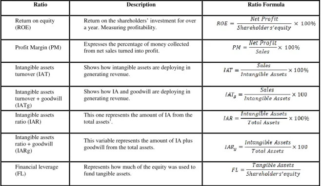
Table 1: Independent and dependent variables description

Ratio Description Ratio Formula

Return on equity (ROE)

Return on the shareholders’ investment for over a year. Measuring profitability.

Profit Margin (PM) Expresses the percentage of money collected from net sales turned into profit.

Intangible assets turnover (IAT)

Shows how intangible assets are deploying in generating revenue.

Intangible assets turnover + goodwill (IATg)

Shows how IA and goodwill are deploying in generating revenue.

Intangible assets ratio (IAR)

This one represents the amount of IA from the total assets1_.

Intangible assets ratio + goodwill (IARg)

This variable represents the amount of IA plus goodwill from the total assets.

Financial leverage (FL)

Represents how much of the equity was used to fund tangible assets.

Source: Author’s own authorship.

Ordinary Least-Squares

The econometric method used in this study to process the selected data was The Ordinary Least-Squares (OLS) method. Heij et al., (2004) described the OLS as the first step in estimating economic relations and could provide a valuable insight into the essence of the relationship between variables. The main objective by using the OLS method is to minimize the remains of the estimated errors. As was said before, the main objective of this study is to identify whether there is a positive effect of IA on the return of the shareholders’ investments of the 68 selected companies on the S&P100 index, as was outlined in the literature review. Since independent variables are presented in the adjusted formula of DuPont, this study fits the independent variables on a multiple linear regression analysis. Of note for this study is that the growth rate of the dependent variable (ROE) is linearly related to the 4 independent variables - profit

margin (PM), IA turnover (AT), IA ratio (AR) and financial leverage (FL). The following formula, Eq. 6, show the OLS equations adapted for the study purposes using the logarithmic function. Indeed, all the previous variables were transformed into are the logarithmic values (lROE, lPM, lIAT, lIAR and lFL) used in each of the formulas. The formula of the OLS analysis follows: (6):

(6)

The formula shows the constant is displayed as the coefficient of the estimator of the population intercept of each independent variable is represented by , the estimation errors are projected by the OLS method and show the impact of each independent variable on the dependent one and the error term, . Lastly, the symbol represents each one of the observations in the dataset, in other words, it represents every single firm in the study’s sample.

In order to keep the results of the OLS in this cross-sectional study unbiased, the model takes the following assumptions: first, the models are linear in their parameters; second, data is a randomly selected sample of the population; third, independent variables are measured exactly such that measurement error is negligible; and, finally, independent variables are not too rigidly collinear.

Results

Descriptive Statistics

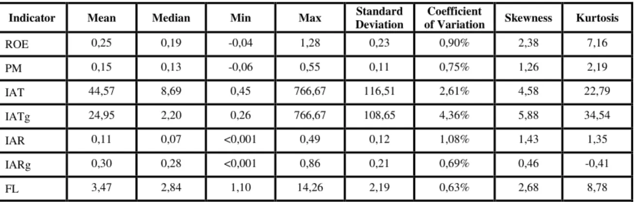
It is necessary to understand the indicator values before this study undertakes an analysis of the results of the OLS Method. Table 2 was elaborated using the sample to provide a clear understanding of the indicators’ distribution of values of the descriptive statistics. Furthermore, indicators of central tendency, variability and shape can be observed in Table 2. The second column presents the statistical mean, which is the most widely used measure of central tendency, while the median, represented in the third column, halves the data. The minimum (min) and the maximum (max) are displayed on the fourth and fifth columns. The standard deviation (the sixth column) and coefficient of variation (seventh column, expressed in percentage) are indicators of dispersion and are both based on the average squared distance between the elements of a data set and the mean. Skewness and kurtosis, in the eighth and ninth columns, are indicators of distribution shape. Kurtosis measures the tailedness and flatness of the normal distribution: in other words, the relative amount of observations in the tails as compared to the number of observations around the mean. Skewness is a measure of the symmetry of the mean for a given studied variable.

Table 2: Descriptive statistics of all variables

Indicator Mean Median Min Max Standard

Deviation

Coefficient

of Variation Skewness Kurtosis

ROE 0,25 0,19 -0,04 1,28 0,23 0,90% 2,38 7,16 PM 0,15 0,13 -0,06 0,55 0,11 0,75% 1,26 2,19 IAT 44,57 8,69 0,45 766,67 116,51 2,61% 4,58 22,79 IATg 24,95 2,20 0,26 766,67 108,65 4,36% 5,88 34,54 IAR 0,11 0,07 <0,001 0,49 0,12 1,08% 1,43 1,35 IARg 0,30 0,28 <0,001 0,86 0,21 0,69% 0,46 -0,41 FL 3,47 2,84 1,10 14,26 2,19 0,63% 2,68 8,78

Note: All values are presented in the same unit of measurement of the variables except the coefficient of variation that is presented in percentage.

The variables “IAT” and “IATg” project the longest distance between their means and maximums. IAT exhibits an outstanding maximum value close to 767% whereas its mean is close to 45%. The distance from the mean to the maximum value is more than 17 times its mean. On the other hand, the minimum values from all the indicators are not far away from their means, with the exception of IAR and IARg. IAT and IATg present the highest values of standard deviation regarding their means. Therefore, their coefficient of variation shows a high degree of dispersion; in particular the result of IATg presented 108,65% of deviation. That means the data for IATg is broadly spread out. Furthermore, these variables present an abnormal skewness, that is to say, their distributions are asymmetric. Additionally, their long right tails mean that the samples are positively skewed; simply put, the data are distributed mainly around the mean. Nevertheless, some data is distant from the mean representing a longer right tail in a graph. The variables’ kurtosis results exhibit a property known as “fat-tails” due to the spread distribution. Fat tails occur where the actual probability of extreme outcomes is greater than the normal distribution: put, in short, the extreme outcomes of the data is expected to be greater than the normal distribution. The variables PM and IAR present low values in contrast with the rest of the variables. Their deviations are close to their respective means and their dispersion is short, as their coefficient of variation is close to 0,8% for the PM and almost 100% for IAR. Kurtosis values are 220% for the PM and for IAR is almost 135%. These results indicate a platykurtic or long tail distribution, meaning that the normal distribution is flat. Regarding the Skewness values, the results show a narrow dispersion around the means.

In summary, all variables are positively skewed due to median values being lower than the means, most of them having maximum values in their data far away from their means (outlier values). Moreover, IAR and PM have narrower dispersions in contrast to IAT and FL. To wit, the variables IAT and PM have values that are close to each other, which is not present in the IAR and FL.

Note that the descriptive statistical analysis showed that some variables present high range values. Therefore, the linear functional form adjusted into a logarithmic functional form has another added advantage. Logarithmic values are known to decrease the degree of dispersion of a variable’s values.

OLS Regression Analysis Results

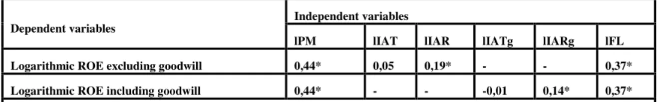
The test is used to assess a possible linear association between two or more variables. For the purpose of this research, the test will help the study to explore which of the 4 independent variables are positively or negatively related to lROE, and the magnitude of such relations. The results of the Pearson correlation coefficient test for all the variables using logarithmic values, see Table 3. The table shows in the first column the name of the logarithmic function of the dependent variables (lROE), for each one of the types of the evaluation values, and the following columns display the independent variables and the results of the Pearson correlation test.

Table 3: Results of the Pearson correlation coefficient between independent variables and the ROE

Dependent variables

Independent variables

lPM lIAT lIAR lIATg lIARg lFL

Logarithmic ROE excluding goodwill 0,44* 0,05 0,19* - - 0,37*

Logarithmic ROE including goodwill 0,44* - - -0,01 0,14* 0,37*

Note. The symbol (*) stands for a 10% level of significance. A set of 66 observations were used to perform this test, two observations presenting negative values were left out. The symbol ( - ) stands for not applicable.

Source: Author’s calculations.

The results show an intense and positive relationship between the logarithmic version of the variables lROE and lPM in comparison to the rest of the independent variables; this means that the observations in the profit margin correspond with observations of lROE. lIAR, lIARg, lIAT and lIATg present low correlation coefficient for ROE. Until this point, the IA recognized in the financial statements show almost insignificant influence on ROE.

The following models, Table 4 and 5, show the regression tests for the dataset selected by this study. The models have been estimated using information from the total sample - 66 companies (two of them were taken out of the test for presenting negative values on the ROE). The format of the tables displays in their first column the adjusted independent variables. The second column shows the results obtained for the estimated coefficients. The third column displays the outcomes of the standard robust errors to assure that the assumption of the homoscedasticity of the error term is not infringed and the results are robust, accurate and it is possible to trust them. The fourth column presents the results of the p-values. This column is related to the fifth column, which indicates the statistical significance of the estimated coefficient. The last column shows the results of the Variance Inflation Factor (VIF). The table correspondingly displays the results for the joint statistical significance test (F-test) and the Adjusted R-squared (adjusted for the degrees of freedom).

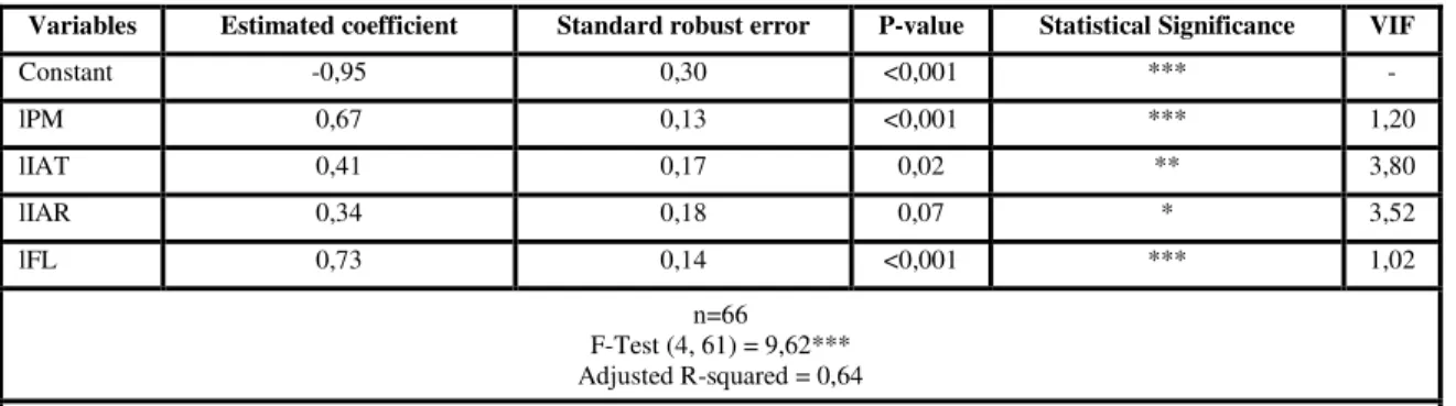
Table 4 : Results of the OLS regression analysis. Excluding goodwill

Variables Estimated coefficient Standard robust error P-value Statistical Significance VIF

Constant -0,95 0,30 <0,001 *** - lPM 0,67 0,13 <0,001 *** 1,20 lIAT 0,41 0,17 0,02 ** 3,80 lIAR 0,34 0,18 0,07 * 3,52 lFL 0,73 0,14 <0,001 *** 1,02 n=66 F-Test (4, 61) = 9,62*** Adjusted R-squared = 0,64

Note. The symbol (***) means 1% level of significance, (**) means 5% of level of significance and (*) means 10% of level of significance. The symbol (-) stands for “not applicable”.

Source: Author’s calculations.

From the results shown in Table 7, it is possible to state that all the estimated coefficients are statistically significant, including the estimated coefficient for the constant. Indeed, with a level of confidence of 99%, it is possible to trust the values computed for the coefficients of the constant, lPM and lFL. With a level of confidence of 95% is possible to trust the value computed for the coefficient of lIAT and with a confidence level of 90% is possible to trust the coefficient computed for the lIAR. This means, for instance, that if the lFL grows 1%, the lROE will grow in the same direction by 0,73%. Regarding the PM if it also grows 1%, it will cause a 0,67% grow in ROE. With respect to lIAT, if it grows 1% the growth in the ROE will be almost 0,4%. Finally, if lIAR increases 1% the lROE will grow 0,35%. The results of the F-test indicate the existence of statistical significance, which means that the variables together compose a good model. This result is supported by the value of the adjusted R-squared. The value of this indicator shows that 64% of the growth on the return on equity is caused by changes that occurred in the independent variables included in the model. Still, 36% of the changes on the return on equity are due to the error term included in the model, this is not explained by the model itself. Finally, it should be noted that the values for the VIF are all smaller than 10, which excludes any collinearity problems among the independent variables.

The following model, Table 5, presents the same format as in the previous table. However, this table presents the logarithmic function of the variables including goodwill.

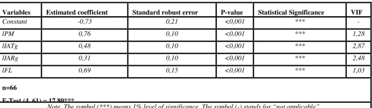
Table 5: Results of the OLS analysis, including goodwill

Variables Estimated coefficient Standard robust error P-value Statistical Significance VIF

Constant -0,73 0,21 <0,001 *** - lPM 0,76 0,10 <0,001 *** 1,28 lIATg 0,48 0,10 <0,001 *** 2,87 lIARg 0,31 0,10 <0,001 *** 2,48 lFL 0,69 0,15 <0,001 *** 1,03 n=66 F-Test (4, 61) = 17,80***

Note. The symbol (***) means 1% level of significance. The symbol (-) stands for “not applicable”.

Source: Author’s calculations.

The Model exhibited in Table 5, shows that all the variables present estimated coefficients with high statistical significance. All independent variables, the constant included, exhibit a level of trustworthiness at 99% for the values computed. The lPM shows the highest estimated coefficient. This is to say that if the variables change 1%, the return on equity will change in the same direction. For the lPM variable, the growth of lROE will grow 0,76%. In the case of lFL, the change will be 0,69%. Concerning lIATg, if it increases 1% the growth in the lROE will be close to 0,48%. Finally, the lIARg presents the weakest effect with 0,31%. That is, that the growth in ROE will be almost 0,30%. The result of the F-test signifies the existence of a statistically significant result, meaning that the variables together comprise a good model. This is supported by the result of the adjusted R-squared. The value of this indicator shows that 72% of the growth on the lROE is caused by changes in the independent variables that were adjusted in the model. Nevertheless, 28% of the changes on the return on the equity are due to the error term included in the model, this is not explained by the model itself. The values of the VIF are presented in the last column, for all variables the results are not higher than 10, this excludes any collinearity problems among the independent variables.

Conclusion

The main purpose of the study was to analyze if the intangible assets, recognized in the balance sheet, have an influence on the return on equity. The literature review showed that, on the one hand, there are studies that indicate a considerable influence of the IA on the ROE, while on the other hand, some studies that did not find a relevant influence. According to our findings, based on the intangible assets ratio (lIAR), the IA has an influence on the return on equity. “IA excluding goodwill” show an influence of 34% on the return on equity; that is, if the IA without goodwill factor grows 1%, the ROE will increase 0,34%. Considering “IA including goodwill”, the ratio lIARg exhibits an influence of 31% on the ROE; it explains almost 0,30% of the growth in ROE when it changes 1%. Therefore, based on the findings of this study, IA recognized on the balance sheet show some influence on the ROE. When the goodwill is included in the IA, the influence on the ROE is 3% lower, because many companies did not disclose goodwill in the balance sheet. Due to “group accounting” and tax planning issues many international companies “hide” their intangible assets in low tax jurisdictions and do not disclose financial information about them.

Acknowledgement

The preparation of the paper was supported by UNIAG, R&D unit funded by the FCT – Portuguese Foundation for the Development of Science and Technology, Ministry of Science, Technology and Higher Education; “Project Code Reference UID/GES/4752/2016”.

References

Artsberg, K. and Mehtiyeva, N. (2010) ‘A literature review on intangible assets’, Dept of Business Administration, (June). Retrieved on 15th May 2018 from https://pdfs.semanticscholar.org/f855/30d9d9b5ad7b7d58e3b8fe855ad2a6553cb3.pdf

Bratianu, C. (2017) ‘The Knowledge Economy: The Present Future’, in Management Dynamics in the Knowledge Economy, 5(4), 477–479. Doi: 10.25019/MDKE/5.4.01.

Bryan, D., Rafferty, M. and Wigan, D. (2017) ‘Capital unchained: finance, intangible assets and the double life of capital in the offshore world’, Review of International Political Economy. Taylor & Francis, 24(1), 56–86. Doi: 10.1080/09692290.2016.1262446.

Cañibano, L., Garcia-Ayuso, M. and Sánchez, P. (2000) ‘Accounting for intangibles: a literature review’,

Journal of Accounting Literature, 19, 102–130.

Carrillo, F. J. (2015) ‘Knowledge-based development as a new economic culture’, Journal of Open Innovation: Technology, Market, and Complexity. Journal of Open Innovation: Technology, Market, and Complexity, 15. 1-15. Doi: 10.1186/s40852-015-0017-5.

Ciurariu, G. (2015) ‘The Du Pont de Nemours System within the Company Diagnostics’, Economy Transdisciplinarity Cognition, 18(2), pp. 25–32.

El-Tawy, N. and Tollington, T. (2013) ‘Some thoughts on the recognition of assets, notably in respect of intangible assets’, Accounting Forum. 37(1), 67–80. Doi: 10.1016/j.accfor.2012.10.001.

Guerard, J. B. and Schwartz, E. (2007) Quantitative corporate finance, Quantitative Corporate Finance. Doi: 10.1007/978-0-387-34465-2.

Heiens, R. A., Leach, R. T. and McGrath, L. C. (2007) ‘The contribution of intangible assets and expenditures to shareholder value’, Journal of Strategic Marketing, 15(2–3), 149–159. Doi: 10.1080/09652540701319011.

Heij, C. et al. (2004) Econometric methods with applications in business and economics. Oxford University Press.

Jensen, M. C. (2008) ‘Erratum: Paying people to lie: The truth about budgeting process (European Financial Management (2003) 9:3 (379-406))’, European Financial Management, 14(2), 375–376. Doi: 10.1111/j.1468-036X.2008.00424.x.

Kijewska, A. (2016) ‘Determinants of the return on equity ratio (ROE) on the example of companies from metallurgy and mining sector in Poland’, Metalurgija, 55(2), 285–288. Doi: UDC – UDK 669.061.5:622.01.061:658.15=111.

Niculita, A. L., Popa, A. F. and Caloian, F. (2012) ‘The Intangible Assets–A New Dimension in The Company’s Success’, Procedia Economics and Finance, 3(12), 304–308. Doi: 10.1016/S2212-5671(12)00156-6.

Pucci, T., Simoni, C. and Zanni, L. (2015) ‘Measuring the relationship between marketing assets, intellectual capital and firm performance’, Journal of Management and Governance, 19(3), 589–616. Doi: 10.1007/s10997-013-9278-1.

Rutkowska-Ziarko, A. (2015) ‘The Influence of Profitability Ratios and Company Size on Profitability and Investment Risk in the Capital Market’, Folia Oeconomica Stetinensia, 15(1), 151–161. Doi: 10.1515/foli-2015-0025.

Saunders, A. and Brynjolfsson, E. (2016) ‘Valuing Information Technology Related Intangible Assets.’,

MIS Quarterly, 40(1), 83–110.

Stockert, P., Kavan, S. and Gruber, M. (2016) ‘What drives Austrian banking subsidiaries ’ return on equity in CESEE and how does it compare to their cost of equity?’, OeNB, Financial Stability Report, 33, 78–88.

Tahat, Y. A., Ahmed, A. H. and Alhadab, M. M. (2017) ‘The impact of intangibles on firms’ financial and market performance: UK evidence’, Review of Quantitative Finance and Accounting, 50(4), 1147-1168. Doi: 10.1007/s11156-017-0657-6.

Vilora, G., Nevado, D. and Lopez, V. R. (2009) Medición y valoración del capital intelectual. Madrid: Pearson Education.

Wittsiepe, R. (2008) IFRS for small and medium-sized enterprises: Structuring the transition process,

IFRS for Small and Medium-Sized Enterprises: Structuring the Transition Process. Springer Science & Business Media. Doi: 10.1007/978-3-8349-9754-8.