A practical approach to parameter
identification for a lightly damped , weakly
non-linear system
Petr Eret
University of West Bohemia, Pilsen, Czech Republic
Craig Meskell
School of Engineering, Trinity College, Dublin, Ireland
Abstract
Fluidelastic systems are often lightly damped and exhibit weak non-linear damping. The weak linear and non-linear damping forces have a significant effect on the long term behaviour of the system. However, parameter identification methods tend to concentrate on identifying the strongest forces. In this paper the applicability of two identification methods to a single degree of freedom fluidelastic system is investigated using experimental data. The system is weakly non-linear under the flow conditions and is prone to the fluidelastic instability (i.e. self excited limit cycle behaviour). The crucial effect of the weak damping forces on the system stability and post-stable behaviour has been demonstrated. The non-linearity detection and identification has been done using an analytic representation of the displacement signal (FREEVIB method) and subsequently a non-linear decrement method was used for comparison. The identified models were used to predict the global behaviour of the system in the form of limit cycle amplitudes and this has been used as an indication of accuracy. It was found that the non-linear decrement method yields superior predictions, but it suffers from the limitation that the functional form of the system must be known a priori. Therefore it is concluded that employing both methods together provides a more powerful approach for parameter estimation in a lightly damped system where weak non-linear damping plays an important role.
Key words: fluidelastic system, parameter identification, weak non-linear damping, analytic signal, decrement method
Email addresses: [email protected](Petr Eret), [email protected](Craig Meskell).
Citation: P Eret & C Meskell, A practical approach to parameter identification for a lightly, Journal of Sound and Vibration, 310, 2008, p829 - 844.
1 Introduction
The identification of non-linear parameters in a lightly damped system is not common in the literature. For example, a recent comprehensive review of iden-tification strategies [1] primarily cites studies concerned with systems exhibit-ing relatively strong non-linearities. The underlyexhibit-ing assumption in many of these approaches is that a weak force does not contribute signifcantly to the overall system dynamics. Indeed, some of the methods simply cannot iden-tify weak non-linear forces due to issues related to poor signal-to-noise ratio (e.g. the reverse path method [2]). However, for some lightly damped sys-tems, the weak linear and non-linear damping forces determine the long term behaviour of the system. Fluidelastic systems are a case in point [3], [4].
Heat exchanger tube arrays are a particular example of this type of fluidelastic system. In this case even a single flexible tube in an otherwise rigid tube array subject to the cross flow of air may experience fluidelastic instability, which is characterized by a rapid increase in vibration amplitude as the flow velocity is increased. These systems have been extensively investigated experimentally. The physical mechanisms have been classified previously by Chen [5]. For a single flexible tube, the mechanism is referred to as a fluid damping controlled instability. The tube motion with a limit cycle oscillation (LCO) can be ob-served at post-stable flow velocities and thus a non-linear model of the coupled fluid-structure system is necessary. The important issue is that the coupled fluid-structure system is very lightly damped and weakly non-linear, but it is these weak damping forces which determine both the onset of instability and the post stable limit cycle amplitude.
phase distortion between the response measurements [13]. In order to avoid these errors, it is desirable to use only a single response measurement of the free response as input to the parameter identification approach.
One possible method to achieve this is the application of the analytic rep-resentation of response signal for a sdof system as shown by Feldman [14] for mono-component free response. The method can detect the non-linear behaviour of the system without an assumption of functional form. The non-linear parameters are estimated directly in this approach. An alternative ap-proach, was proposed by Meskell [15] and is based on consideration of the amplitude decrement between periods of the system response. However, this method requires knowledge of the type of non-linearity present. In this paper the decrement method has been slightly modified to achieve more accurate results and a numerical simulation has been conducted to verify the reliability of this enhanced method.
The overall objective of the work is to demonstrate the applicability of these two methods of non-linear parameter estimation to experimental data for a lightly damped system with very weak damping non-linearities, and hence define a robust methodology for system identification of these types of system.
2 Experimental setup
The investigated fluidelastic system is a five row normal triangular array of 38 mm diameter tubes with a pitch ratioP/d= 1.32 as shown in Fig. 1. All tubes were rigidly supported except the central one in the third row (shaded in Fig. 1), which was mounted on a elastic support with the possibility of traverse displacement (y) only. It has been verified experimentally that this support behaves as a linear sdof system in quiescent air for the range of displacement considered and the oscillating mass is approximately 1 kg. The structural damping is controlled using a passive electro-magnetic damper. Thus, linear damping modification is independent of system mass and structural stiffness. Under flow conditions the system is weakly non-linear as will be apparent from following sections. More details of the experimental setup can be found in reference [10].
structural damping, where δ =πc/Ω with cas a mass normalized coefficient of the structural damping and Ω as a system natural frequency. At flow veloc-ities higher than the critical flow velocity the tube motion is not dynamically divergent as would be indicated by a purely linear system. The amplitude of the tube motion is limited. No hysteretic behaviour of the stability threshold with the flow velocity has been observed. The drop around a flow velocity of 9 m/s is due to an acoustic resonance [10] and will not be considered here.
3 System identification
Two methods have been applied to estimate mass normalized parameters of the investigated system using only a single response measurement. The first method based on analytic signal can detect a non-linear behaviour of a sdof system and identify parameters. This method is more complicated to imple-ment and requires digital filtering to smooth the input signal and remove ex-traneous noise. The second method is a non-linear decrement method, which is limited to lightly damped systems. For completeness both techniques are briefly described below in sections 3.1 and 3.3.
3.1 Method using analytic signal
An analytic representation of a real signal has wide applications in data pro-cessing. An analytic approximation of a signal is usually associated with the Hilbert transform in the time domain. It is well known that the Hilbert trans-form is related to the Fourier transtrans-form (FFT) in the frequency domain. A simple example can be found in Marple[16], which describes a method to cre-ate a standard discrete time analytic signal, with the same sample rcre-ate and frequency content as the original data, by setting the second half of the fre-quency spectrum to zero. A method using analytic signal for a non-linearity detection and identification of a sdof system in free response has been proposed by Feldman [14].
Equation (1) defines an analytic signalY(t) in terms of a real party(t) (which is the original data) and an imaginary part ˜y(t) computed using the Hilbert transform,H[y(t)] = ˜y(t). The Hilbert transform behaves as a 90◦ phase shift filter
Y(t) =y(t)−y˜(t). (1)
y(t) =A(t) cos(ψ(t)), (2) ˜
y(t) =−iA(t) sin(ψ(t)), (3)
where A(t) and ψ(t) are the instantaneous amplitude and phase, respec-tively. The time derivates using relations A(t) = y(t)2−y˜(t)2 and ψ(t) = arctan(iy˜(t)/y(t)) can be obtained
˙
A(t) =y(t) ˙y(t)−y˜(t) ˙˜y(t)
A(t) , (4)
ω(t) = ˙ψ(t) =iy(t) ˙˜y(t)−y˙(t)˜y(t)
A(t)2 , (5)
where ω(t) is an instantaneous frequency of a real signal.
The first and second time derivatives of the analytic signal Y(t) are
˙
Y(t) =Y(t)
˙ A(t)
A(t)+iω(t)
, (6)
¨
Y(t) =Y(t)
¨ A(t)
A(t)−ω(t)
2+i2A˙(t)ω(t)
A(t) +iω˙(t)
. (7)
Now consider the mass normalized equation of motion for a sdof system, Eq.(8), where b(t) and Ω(t) are the instantaneous damping and natural fre-quency, respectively. The application of the Hilbert transform to this equation will yield Eq.(9) providing that the signal y(t) (and its derivatives) has a high frequency content compared the functions b(t) and Ω2(t). In essence, this re-quires that the damping and stiffness change slowly in time compared to the periodic time of the data,y(t).
¨
y+b(t) ˙y+ Ω2(t)y= 0, (8)
¨˜
y+b(t) ˙˜y+ Ω2(t)˜y= 0. (9)
In the type of system of interest here (i.e. a weak non-linearity in damping)
b(t) is almost constant in time, while ˙y(t) describes the system motion at a relatively high natural frequency. Thus, these two signals will have non-overlapping spectra. Using the main properties of the Hilbert transform it can be shown easily that H[b(t) ˙y] = b(t)H[ ˙y] = b(t) ˙˜y. Similar reasoning can be applied to Ω2(t) and y(t).
transformed data:
¨
Y +b(t) ˙Y + Ω2(t)Y = 0. (10)
Substituting Eqs.(6) and (7) into Eq.(10) and separating the real and imag-inary parts gives mass normalized coefficients of damping b(t) and stiffness Ω2(t)
b(t) =−2 ˙
A(t)
A(t)− ˙
ω(t)
ω(t), (11)
Ω2(t) =ω(t)2− ¨
A(t)
A(t) + 2 ˙
A(t)2
A(t)2 + ˙
A(t) ˙ω(t)
A(t)ω(t). (12)
The instantaneous system damping force and stiffness force, fD and fS, re-spectively, can be expressed as
fD =b(t)ω(t)A(t), (13)
fS = Ω2(t)A(t). (14)
To explore a non-linearity in the damping and stiffness characteristics of the system it is convenient to plot a damping forcefD against a velocity amplitude
ω(t)A(t) and a stiffness force fS against a displacement amplitude A(t). As errors can be expected in both axis, a total least square approach is used to obtain estimates of the linear and non-linear parameters by simply fitting an appropriate function to the data.
3.2 Experimental results for method using analytic signal
As the system under investigation is weakly non-linear, no harmonics can be found in the measured displacement response. A narrow bandpass digital filtering, which was suggested as a part of the applied method [14], is required to eliminate noise away from the primary response. This is necessary to ensure numerical differentiation of the free decay displacement yields reliable time derivations of the signal. Thus a narrow band-pass filter has been applied to the displacement signal to get a response in the area around the natural frequency of 6.6 Hz of the first structural mode (the natural frequency of the second tranverse mode is above 77 Hz). An elliptic IIR filter of sixth order with an exact stop-band matching (band ripple of 0.01 dB) and pass-band of 6Hz-8Hz was used. The original method by Feldman also proposed a low-pass filtering of the calculated instantaneous signalsb(t),Ω2(t), A(t), ω(t). A 3rd order Chebyshev 2 IIR filter with a cutoff frequency of 40 Hz and an attenuation of 100 dB in the stopband has been applied. All filters have an impulse response amplitude below 1×10⁻⁵ after a time of 2 second.
In order to eliminate the effect of the initial transients of the digital filters, the reversed time sequence displacement signal has been used for the applica-tion of the method, since a higher order non-linearity is most obvious at the higher amplitudes of the oscillations. In this way filter transients are displayed at lower amplitudes. This corrupted data is discarded from the calculations. Although this step leads to better non-linearity detection and identification, it does mean that the filtering process is acausal. This does not represent a major limition, however, as parameter identifcation is usually executed offline.
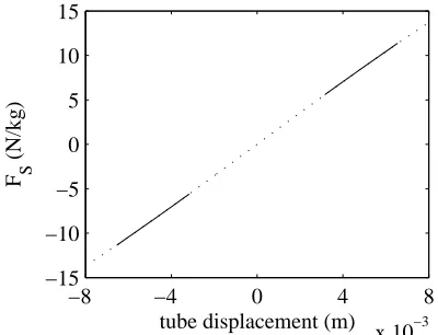
The stiffness and damping characteristics of the fluidelastic system have been obtained using the application of the FREEVIB method described above. At zero flow velocity the investigated system is considered to have the linear characteristics as shown in Fig. 3 for damping and in Fig. 4 for stiffness. Strictly speaking, the analysis showed negligible, but not zero, structural non-linear forces (negative cubic stiffness and damping). This can be attributed to numerical and quantization errors. As the flow velocity increased, weak non-linearities with cubic form appeared. The cubic form in damping at the flow velocity of 4 m/s is more visible as can be seen in Fig. 5. The softening stiffness at the same flow velocity in given in Fig. 6, it is less apparent, but the regression analysis indicates its presence. This reflects the relative magnitude of the structural stiffness compared to the fluidelastic stiffness. At the last investigated flow velocity of 8.5 m/s the non-linear cubic characteristics of the fluidelastic system are most obvious as shown for the damping in Fig. 7 and the stiffness in Fig. 8.
linear fluid stiffness (Fig. 10), since an added mass can be neglected in the case of the air. The non-linear cubic fluid stiffness in Fig. 11 has increasing softening effect. The damping has a crucial role in the stability of this system. The Fig. 12 shows the increasing negative linear fluid damping, which results in decreasing total damping of fluidelastic system, in the case of zero total damping the stability threshold occurs. The non-linear cubic fluid damping, which determines the post-stable amplitude, is shown in Fig. 13.
3.3 Decrement method
A method to estimate the damping parameters for lightly damped systems with a weak non-linearity has been proposed by Meskell [15]. This section details the main principle of the method and introduces a slight modification to achieve more accurate results. The modified method is verified using a numerical simulation initially, before being applied to the experimental data.
The mass normalized equation of motion of system in free response is
¨
y+fD(y,y˙) + Ω2y = 0, (15)
where Ω =
k/m and fD is the mass normalized damping force includ-ing both linear and non-linear dampinclud-ing. The free response is assumed to be sinusoid with time varying amplitude A(t) and natural angular frequency Ωd = Ω√1−D2 where Dis a damping ratio
y(t) = A(t) cos(Ωdt+φ). (16)
If the damping is weakD2 1 (i.e. Ωd≈Ω) and the change of amplitude dur-ing short time period is small (i.e. ˙A≈0), then the velocity and acceleration can also be assumed to be sinusoidal.
The mass normalized instantaneous mechanical energy in the system can be written as,
e(t) = 1 2Ω
2y2(t) + 1
2y˙
2(t). (17)
Substituting system displacement and velocity into Eq.(17) relates the instan-taneous specific energy to the instaninstan-taneous amplitude of vibration
e(t) = 1 2Ω
Alternatively, the specific energy can be obtained by considering the energy dissipated by the damping forcefD. The instantaneous energy is simply
e(t) =e0(t)−wD(t), (19)
wheree0 is the initial energy at t= 0. The specific work done by the damping force is
wD(t) = t
0
fD(τ) ˙y(τ)dτ. (20)
Combining Eqs.(18), (19) and (20) yields
A2(t) = A20− 2 Ω2
t
0
fD(τ) ˙y(τ)dτ, (21)
whereA0 is the amplitude att= 0. Substituting the system velocity, changing the variable in the integral to θ = Ωτ +φ and evaluating this equation over one period of vibration yields the basic equation for the decrement method
A21 =A20− 2 Ω3
2π
0
fD(θ) ˙y(θ)dθ. (22)
In previous section the form of non-linear damping force of the fluidelastic system has been identified as cubic from experimental data. Thus, the total damping force including non-linear and linear part is given by
fD =cy˙+βy˙3. (23)
Note that the damping coefficients are already mass normalized. Assuming a constant response amplitude ofAc, the work done over one period of vibration is
2π
0
fD(θ) ˙y(θ)dθ=cA2c
2π
0
Ω2cos2(θ)dθ+βA4c
2π
0
Ω4cos4(θ)dθ
=cA2cΩ2π+βA4cΩ43π
4 . (24)
Combining this with Eq.(22) yields
where
λ1 = 2π
Ωc, (26)
λ2 = 3πΩ
2 β. (27)
In this study it is assumed, that the constant amplitude Ac is simply the average of the initial and final amplitudes in one period, which should elim-inate accumulated errors (compare Meskell [15], where the initial and final amplitudes were used to yield two sets of parameter estimates)
Ac =
1
2(A0 +A1). (28)
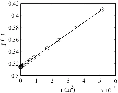
Substituting Eq.(28) into Eq.(25) and rearranging yields an equation for a straight line
p=λ1+λ2r, (29)
where
r=
A0
2 +
A1
2
2
, (30)
p= (A
2 0−A21)
r . (31)
Note theA0,A1 pairs are known from the response data. Once again, a total least square approach is used for parameters λ1 , λ2 estimation since errors are expected in both variables p and r.
3.4 Experimental results for decrement method
The displacement free decay responses at each flow velocity were smoothed using an acausal band pass filter with zero-phase distortion. This filter has precisely zero phase distortion and minimal magnitude attenuation in the pass band.
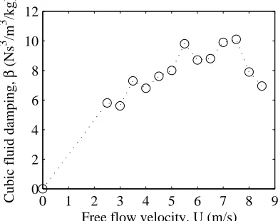
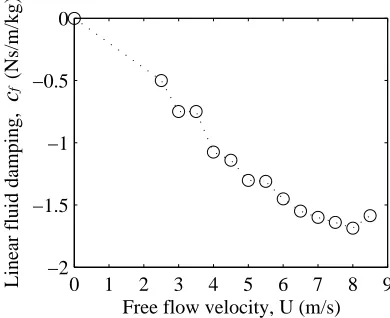
Using this technique the information about system damping is available. As can be seen in Fig. 15 the linear fluid damping is negative and Fig. 16 shows positive non-linear cubic fluid damping, which seems to reach a constant value again within flow velocity range from 3 to 7.5 m/s. This effect is hard to explain physically. However, as will be seen below, the good prediction of overall system behaviour (i.e. LCO amplitude) supports this trend in the cubic damping parameter. Further study into this problem is required to isolate the fluid mechanism responsible and is beyond the scope of this study.
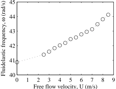
The drop in parameter values at the last flow velocity can be attributed to an interaction with acoustic resonance. The increase in fluidelastic frequency is due to fluidelastic stiffness as shown in Fig. 17 which has been obtained from averaged steady peak periods. The information about non-linear fluid stiffness is unknown using the decrement method. However, as will be demonstrated below, the non-linear fluid stiffness does not play an important role in the dynamics of this fluidelastic system.
3.5 Prediction of post-stable response
A criterion of good parameter estimates of linear and non-linear damping from both applied techniques is the prediction of the stability thresholds and the post-stable behaviour. In post-stable regimes fluidelastic systems establishes a limit cycle oscillation (LCO) with constant amplitude at a given flow velocity. The total work during one period is zero as shown in [10] is a function of the damping coefficients and fluidelastic frequency only, since all stiffness forces are conservative. The limit cycle amplitude is expressed as
ALCO =
−4
3
cf(U) +cs
β(U)Ω2(U), (32)
where all parameters have been experimentally determined previously, cf is linear fluid damping coefficient, β is non-linear cubic fluid damping coeffi-cient and Ω is fluidelastic frequency, all as a function of flow velocity U;
cs is structural damping coefficient independent on flow velocity U. Using
cy-cle amplitudes can be predicted for the system with lower damping levels
δ= [0.093,0.106,0.114] assuming the same trends for the fluid coefficients.
Comparing the predicted response amplitudes, obtained using the identified linear and non-linear coefficients, with experimental response amplitudes for the same system damping (Fig. 2) offers a measure of the accuracy of the identification methods. Tab. 3 compares the two sets of predictions for the critical velocity with the directly measured experimental values. Tab. 4 com-pares the predicted and experiemntal rms response of the system at three levels of damping for a flow velocity of 8m/s.
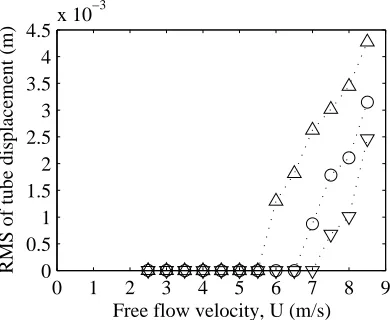
The rms levels for the system predicted using the analytic signal method (FREEVIB) is shown in Fig. 18. The estimates of the critical velocity are consistently overestimated (Tab. 3), implying a systematically low value of the estimated linear fluid damping . The trend of the post-stable behaviour is in satisfactory agreement with the experimental data but the amplitudes are a slightly overestimated (Tab. 4). As the LCO amplitude depends on the ratio of the linear to the cubic damping and so this implies, that the cubic damping is also underestimated.
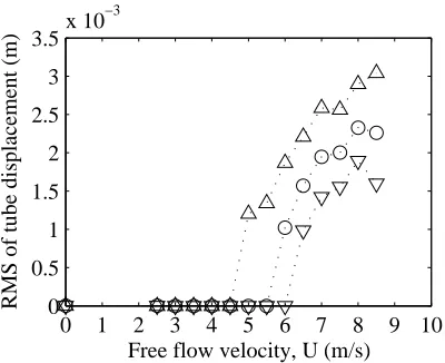
The decrement method (Fig. 19) gives better predictions of the critical flow velocities (Tab. 3), although there are still slightly overestimated. This implies a superior estimation of the linear fluidelastic damping compared to FREE-VIB. The post-stable amplitudes are also predicted reasonably well (Tab. 4) and the trend is in a good agreement to the experimental data.
Thus, it is appears that the decrement method yields superior estimates of the damping parameters, both linear and non-linear, for this type of system, although it should be noted that the functional form of the non-linearity must be assumed.
4 Conclusions
signal-to-noise ratio. With this in mind, two different methods which are suited to this type of situation, have been applied to estimate system parameters and to predict the post-stable behaviour with stability threshold. The results show that each technique has a specific advantage. The method using an analytic signal (FREEVIB) can detect the non-linear behaviour of a system without prior knowledge of the functional form and subsequently the non-linear decre-ment method can be used to achieve more accurate parameter estimates as verifying by the prediction of global behaviour (i.e. limit cycle amplitudes). Therefore, it is concluded that the application of the both methods together provides a powerful tool for parameter estimation of a sdof system, where a weak non-linear and linear damping play an important role.
5 Acknowledgement
This work has been supported by the European Doctorate in Sound and Vi-bration Studies funded under the Marie Curie multipartner training site pro-gramme (Contract Number MEST-CT-2004-503675).
References
[1] Kerschen, G., Worden, K., Vakakis, A.F., and Golinval, J-C., “Past, present and future of nonlinear system identification in structural dynamics”. Mechanical Systems and Signal Processing,20(3), 2006, pp. 505–592.
[2] Rice, H. J., Fitzpatrick, J.A. “A generalized technique for spectral analysis of non-linear systems”. Mechanical Systems and Signal Processing, 2, 1988, pp. 195–207.
[3] Marsden, C.C., Price, S. J., “The aeroelastic response of a wing section with a structural freeplay nonlinearity: An experimental investigation”. Journal of Fluids and Structures, 21(3), 2005, pp. 257-276.
[4] Nakamura, T., “ON TREATMENT OF NONLINEAR DAMPING FOR OCCURRENCE OF DAMPING-CONTROLLED FLUID-ELASTIC INSTABILITY” ASME Pressure Vessels and Piping Division Conference, Vancouver, BC, edited by M.P.P. Paidoussis , ASME, 2006, PVP2006-ICPVT11-93772
[5] Chen, S. S., “Instability mechanisms and stability criteria of a group of circular cylinders subjected to cross-flow. Part I: Theory”.Journal of Vibration, Acoustics, Stress and Reliability in Design,105 (51), 1983, pp. 51–58.
Table 1
System parameter values.
Ω2 (rad/s)2 c (Ns/m/kg) β (Ns3/m3/kg)
1600 2 10
[7] Rzentkowski, G., and Lever, J.H., “Modeling of the nonlinear fluidelastic behaviour of a tube bundle”. In:Paidoussis, M.P., Chen, S.S., Steiniger, D.A. (Eds.), Cross Flow Induced Vibration of Cylinder Arrays. ASME, New York, 1992, pp. 89–106.
[8] Rzentkowski, G., and Lever, J.H., “An effect of turbulence on fluidelastic instability in tube bundles: a nonlinear analysis”. Journal of Fluids and Structures,12, 1998, pp. 561–590.
[9] Lever, J.H., and Weaver, D.S., “A theoretical model for fluidelastic instability in heat exchanger tube bundles”.ASME Journal of Pressure Vessel Technology, 104, 1982, pp. 147–158.
[10] Meskell, C., and Fitzpatrick, J.A., “Investigation of the nonlinear behaviour of damping controlled fluid-elastic instability in a normal triangular tube array”. Journal of Fluids and Structures,18(5), 2003, pp. 573–593.
[11] Masri, S., and Caughey, T., “A non-parametric identification technique for nonlinear dynamic problems.”. Journal of Applied Mechanics, 46, 1979, pp. 433–447.
[12] Worden, K., “Data processing and experiment design for the restoring force surface method. part 1: Integration and differentiation of measured time data. part 2: Choice of excitation signal”. Mechanical Systems and Signal Processing, 4, 1990, pp. 295–344.
[13] Meskell, C., and Fitzpatrick, J.A., “Errors in parameter estimates from the force state mapping technique for free response due to phase distortion”. Journal of Sound and Vibration, 252(5), 2002, pp. 967–974.
[14] Feldman, M., “Non-linear system vibration analysis using Hilbert transform– I. Free vibration analysis method ’FREEVIB’ ”. Mechanical System Signal Processing,8, 1994, pp. 119–127.
[15] Meskell, C., “A decrement method for quantifying non-linear and linear damping parameters”.
Journal of Sound and Vibration,296 (3), 2006, pp. 643–649.
P (=50mm)
d (=38mm) U
[image:15.612.147.438.34.191.2]x y
Fig. 1. Schematic of tube array P/d=1.32 taken from [10].
0 1 2 3 4 5 6 7 8 9 10
0 0.5 1 1.5 2 2.5 3 3.5x 10
−3
Free flow velocity, U (m/s)
[image:15.612.190.387.246.407.2]RMS of tube displacement (m)
Fig. 2. RMS of tube motion at three levels of damping: Δ, δ= 0.093; ◦,δ = 0.106; ∇,δ = 0.114 taken from [10].
−0.4 −0.2 0 0.2 0.4
−0.8 −0.4 0 0.4 0.8
tube velocity (m/s)
F D
(N/kg)
[image:15.612.188.387.477.634.2]−8 −4 0 4 8
x 10−3 −15
−10 −5 0 5 10 15
tube displacement (m)
F S
[image:16.612.189.388.35.188.2](N/kg)
Fig. 4. Structural stiffness at U = 0 m/s:−, experimental data;· · ·, linear fitting.
−0.4 −0.2 0 0.2 0.4
−0.8 −0.4 0 0.4 0.8
tube velocity (m/s)
F D
[image:16.612.188.387.245.398.2](N/kg)
Fig. 5. Total damping at U = 4 m/s including structural and fluidelastic components: −, experimental data;· · ·, cubic fitting.
−8 −4 0 4 8
x 10−3 −15
−10 −5 0 5 10 15
tube displacement (m)
F S
(N/kg)
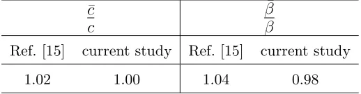
[image:16.612.188.388.466.619.2]Table 2
Linear and non-linear cubic damping parameter.
¯
c c
¯
β β
Ref. [15] current study Ref. [15] current study
[image:17.612.144.429.214.292.2]1.02 1.00 1.04 0.98
Table 3
Experimental and predicted critical velocities (m/s).
Structural viscous damping,δ
0.093 0.106 0.114
Experiment 4.0 5.5 6.5
FREEVIB [14] 5.5 6.5 7.0
Decrement Method [15] 4.5 5.5 6.0
Table 4
Experimental and predicted rms levels at a velocity of 8m/s (mm).
Structural viscous damping,δ
0.093 0.106 0.114
Experiment 2.6 2.1 1.8
FREEVIB [14] 3.5 2.1 1.0
Decrement Method [15] 2.8 2.2 1.8
−0.4 −0.2 0 0.2 0.4
−0.8 −0.4 0 0.4 0.8
tube velocity (m/s)
F D
(N/kg)
[image:17.612.158.420.356.627.2] [image:17.612.147.430.364.441.2]−8 −4 0 4 8
x 10−3 −15
−10 −5 0 5 10 15
tube displacement (m)
F S
[image:18.612.188.388.37.190.2](N/kg)
Fig. 8. Total stiffness at U = 8.5 m/s including structural and fluidelastic compo-nents: −, experimental data;· · ·, cubic fitting.
0 1 2 3 4 5 6 7 8 9
40 41 42 43 44 45
Free flow velocity, U (m/s)
Fluidelastic frequency,
ω
[image:18.612.190.388.265.417.2](rad/s)
Fig. 9. Fluidelastic frequency.
0 1 2 3 4 5 6 7 8 9
0 50 100 150 200 250 300
Free flow velocity, U (m/s)
Linear fluid stiffness,
k f
(N/m/kg
)
[image:18.612.189.387.477.633.2]0 1 2 3 4 5 6 7 8 9 −2
−1.6 −1.2 −0.8 −0.4
0x 10 6
Free flow velocity, U (m/s)
Cubic fluid stiffness,
η
(N/m
[image:19.612.191.385.39.198.2]3 /kg)
Fig. 11. Mass normalized non-linear cubic fluid stiffness.
0 1 2 3 4 5 6 7 8 9
−2 −1.5 −1 −0.5 0
Free flow velocity, U (m/s)
Linear fluid damping,
c f
(Ns/m/kg
[image:19.612.186.387.258.416.2])
Fig. 12. Mass normalized linear fluid damping.
0 1 2 3 4 5 6 7 8 9
0 2 4 6 8 10 12
Free flow velocity, U (m/s)
Cubic fluid damping,
β
(Ns
3 /m
3 /kg
)
[image:19.612.191.386.475.630.2]0 1 2 3 4 5 6
x 10−5 0.3
0.32 0.34 0.36 0.38 0.4 0.42
r (m2)
[image:20.612.190.388.256.412.2]p (−)
0 1 2 3 4 5 6 7 8 9 −2
−1.5 −1 −0.5 0
Free flow velocity, U (m/s)
Linear fluid damping,
c
f
(Ns/m/kg
[image:21.612.190.385.256.415.2])
0 1 2 3 4 5 6 7 8 9 0
5 10 15 20 25 30
Free flow velocity, U (m/s)
Cubic fluid damping,
β
(Ns
3 /m
3 /kg
[image:22.612.191.387.39.195.2])
Fig. 16. Mass normalized non-linear cubic fluidelastic damping.
0 1 2 3 4 5 6 7 8 9
40 41 42 42 44 45
Free flow velocity, U (m/s)
Fluidelastic frequency,
ω
[image:22.612.191.387.251.404.2](rad/s)
Fig. 17. Fluidelastic frequency.
0 1 2 3 4 5 6 7 8 9
0 0.5 1 1.5 2 2.5 3 3.5 4 4.5x 10
−3
Free flow velocity, U (m/s)
RMS of tube displacement (m)
Fig. 18. Predicted RMS of tube displacement using analytic signal: Δ, δ = 0.093;
[image:22.612.191.386.460.620.2]0 1 2 3 4 5 6 7 8 9 10 0
0.5 1 1.5 2 2.5 3 3.5x 10
−3
Free flow velocity, U (m/s)
[image:23.612.189.389.246.409.2]RMS of tube displacement (m)
Fig. 19. Predicted RMS of tube displacement using decrement method: Δ,δ = 0.093;
![Fig. 1. Schematic of tube array P/d=1.32 taken from [10].](https://thumb-us.123doks.com/thumbv2/123dok_us/1491089.689342/15.612.188.387.477.634/fig-schematic-tube-array-p-d-taken.webp)