D S Sharma, R Sangal and A K Singh. Proc. of the 13th Intl. Conference on Natural Language Processing, pages 71–80, Varanasi, India. December 2016. c2016 NLP Association of India (NLPAI)
Dependency grammars as Haskell programs
Tomasz Obr˛ebski
Adam Mickiewicz University Pozna´n, Poland
Abstract
In the paper we try to show that a lazy functional language such as Haskell is a convenient framework not only for imple-menting dependency parsers but also for expressing dependency grammars directly in the programming language in a com-pact, readable and mathematically clean way. The parser core, supplying neces-sary types and functions, is presented to-gether with two examples of grammars: one trivial and one more elaborate, allow-ing to express a range of complex gram-matical constraints such as long distance agreement. The complete Haskell code of the parser core as well the grammar exam-ples is included.
1 Introduction
Functional programming is nowadays probably the most rapidly developing subfield in the domain of theory and implementation of programming languages. Functional languages, with Haskell as their flagship, are continuously evolving, mostly by absorbing more and more mathematics (ab-stract algebra, category theory). This translates into their increasing expressiveness, which is di-rectly usable by programmers.
The combination of keywords functional
pro-grammingandparsingusually brings to mind the
monadic parsing technique (Hutton and Meijer, 1998) developed as an attractive functional of-fer for parser builders. This technology is ded-icated mostly to artificial languages. Much less work has been done in functional programming paradigm regarding natural language parsing tech-nologies. The outstanding exception is the
Gram-matical Framework environment (Ranta, 2011).
Written in Haskell with extensive use of higher-order abstraction and laziness property, it offers
impressive capabilities of making generalizations in all conceivable dimensions in a large and highly multilingual language model including morpho-logical, syntactic and semantic layers. Some other works, which may be mentioned here, are due to Ljunglöf (2004), de Kok and Brouwer (2009), Ei-jck (2005).
As far as dependency-based parsing and lan-guage description is concerned (Kubler et al., 2009), the author is not aware of any attempts to apply functional programming techniques.
Below we try to show that a lazy functional lan-guage such as Haskell is a convenient framework not only for implementing dependency parsers but also for expressing dependency grammars directly as Haskell code in a compact, readable, and math-ematically clean way.
semirings (cf. Goodman, 1999), to mention just two.
2 The Haskell toolbox
Haskell is a purely functional programming lan-guage, applying lazy evaluation strategy, see (Jones, 2002) for language specification, (Lipo-vaca, 2011) for introductory course, and (Yorgey, 2009) for information on advanced Haskell alge-braic type classes. We will take a closer look at two Haskell types on which the parser and gram-mar implementation is based:
[a] – list of elements of typea
a→[a]– a function taking an argument of type aand returning a list of el-ements of typea.
Below, we are going inspect the properties of those types as well as functional tools which will allow us to operate on them conveniently.
Lists are used to store collections of values. Their interpretation depends on the context. We use lists for representing sequences, sets, alterna-tives of values as well as possible lack of a value (singleton list - value exists, empty list - no value). The other important type is the type of functions that take an argument of some typea and return a list of values of type a, i.e. the type a→[a]. These are functions which return sequences, sets, alternatives, or a possibly lacking value, all repre-sented by lists. Here are some examples:
• the function which extends the parse with a
new node produces several alternative results for the word "fly" (typeParse→[Parse]);
• the function returning the preceding node
has no value for the first node (type
Node→[Node]);
• the function computing transitive heads
of a node returns a set of nodes (type
Node→[Node]).
A list type [a]is obtained by applying the list functor[]to some typea, with no constraints on whatais. Two properties are particularly useful: (1) the list functor[]is an instance ofMonad; (2) a list of elements of any type is an instance of
Monoid.
Functions and operators from both classes
(Monoid and Monad) may be intermixed for lists
because they share the value-combining operation: both thejoin1operation in the list monad and the
operation in the monoid[a]is concatenation. An important consequence of the fact that[a] is an instance ofMonoid is that all functions which re-turn[a]are also instances ofMonoid. Below we summarize the list of operators on values of type
[a]anda -> [a], supplied by classesMonadand
Monoid, which we will make use of.
• ⊕::[a]→[a]→[a]
(instance Monoid [a])
xs⊕yscombines values contained inxswith those in ysproducing one list with both xs andys;
• ⊕::(a→[a])→(a→[a])→(a→[a])
(instance Monoid (a -> [a]))
f⊕gcombines functionsfandg, which both return a list of values of typea, into a single function returning one list that contains the return values of bothfandg;
• >=>::(a→[a])→(a→[a])→(a→[a])
(instance Monad [])
f >=> g composes functionsf andgin one
function (of the same type). The resulting function appliesgto each value from the list returned by f and returns the results com-bined in one list;
• >>=::[a]→(a→[a])→[a]
(instance Monad [])
[a] >>= f applies f to all values from [a]
and combines the results.
In addition to the operators listed above, we will use the function:
• pure::a→[a]
(instance Applicative [])
which returns a singleton list containing its argument. It is equivalent to the monadic
return function, but it reads much better in
our contexts.
Having a function of type a→[a], we will be frequently also interested in its transitive closure or reflexive transitive closure (strictly speaking -the termtransitive closurerefers to the underlying
1The operation which transforms a list of lists into a flat
relation). We will introduce the family of closure functions. They are used for example to obtain the function which computes transitive heads from the function that returns the head.
clo,mclo,rclo,mrclo::(a→[a])→a→[a] clo f = f >=> ( pure⊕clo f ) rclo f = pure⊕clo f
mclo f = f >=> mrclo f
mrclo f x = let fx = f x in if null fx then pure x
else fx >>= mrclo f
The function clo computes the closure of its argument function f. The functionf is (Kleisli) composed with the function which combines (⊕)
its arguments (purevalues off) with the values of recursive application ofclo fon each of those ar-guments. The functionrclocomputes the reflex-ive transitreflex-ive closure of its argument function f. The argument itself (pure) is combined (⊕) with the values returned byclo fapplied to this argu-ment. Them*versions ofcloandrcloreturn only maximal elements of closures, i.e. those for which the argument functionfreturns no value.
The operators and functions presented above will be expecially useful for working with rela-tions. This is undoubtedly the most frequently used mathematical notion when talking about de-pendency structures. We use relations to express relative position of a word (node) with respect to another word (predecessor, neighbor, dependent, head). We also frequently make use of such oper-ations on reloper-ations as transitive closure transitive head, reflexive transitive dependent) or composi-tion (transitive head of left neighbour).
Haskell is a functional language. We will thus have to capture operations on relations by means of functions. The nearest functional relatives of a relation are image functions.
Given a relationR ⊂ A×B, the image func-tionsR[·]are defined as follows (1 – image of an
element, 2 – image of a set):
(1) R[x] = {y|xRy} wherex∈A (2) R[X] = {y|x∈X∧xRy} whereX⊂A
Haskell expressions corresponding to image functions and their use are summarized below (x has typea, xs has type [a], rand shave type
a →[a]):
R[x] r x (or pure x >>= r)
R[X] xs >>= r
(R◦S)[·] s >=> r
(R∪S)[·] r⊕s
R+[·] clo r
R∗[·] rclo r
3 Data structures
The overall design of the parser is traditional. Words are read from left to right and a set of alter-native parses is built incrementally. We start with describing data types on which the parser core is based. They are designed to fit well into the func-tional environment2.
3.1 TheParsetype
A (partial) parse is represented as a sequence of parse steps. Each step consumes one word and in-troduces a new node to the parse. It also adds all the arcs between the new node and the nodes al-ready present in the parse. All the data added in a parse step – the index of the new node, its cat-egory and the information on its connections with the former nodes – will be encapsulated in a value of typeStep:
type Parse = [Step]
data Step = Step Ind Cat [Arc] [Arc] deriving (Eq,Ord)
A value of type Step is built of the type con-structor of the same name and four arguments:
(1) the word’s index of typeInd. It reflects the position of the word in the sentence. It is also used as the node identifier within a parse;
(2) the syntactic category of the node represented by a value of typeCat;
(3) the arc linking the node to its left head. This value will be present only if the node is pre-ceded by its head in the surface ordering. List is used to represent a possibly missing value.
(4) the list of arcs which connect the node with its left dependents.
We also make Step an instance of the classes EqandOrd. This will allow us to use comparison operators (based on node index order) with values of typeNodeintroduced below.
The value of typeArcis a pair:
2The functional programming friendly representation of a
type Arc = (Role,Ind)
whereIndis the integer type.
type Ind = Int
For the sentenceJohn saw Mary. we obtain the following sequence of the parse steps:
[ Step 3 N [(Cmpl,2)] [], Step 2 V [] [(Subj,1)], Step 1 N [] [] ]
We introduce three operators for constructing a parse:
infixl 4 <<, +->,
+<-(<<) :: Parse -> (Ind,Cat) -> Parse p << (i,c) = Step i c [] [] : p
(+->),(+<-) :: Parse -> (Role,Ind) -> Parse (Step i c [] d: p) +-> (r,j) = Step i c [(r,j)] d : p (Step i c h d: p) +<- (r,j) = Step i c h ((r,j):d) : p
The operator<<adds an unconnected node with indexiand category cto the parsep. The
oper-ator +->links the node i as the head of the
cur-rent (last) node with depencency of typer. The operator+<-links the nodeias the dependent of the current node with depencency of type r. All the operators are left associative and can therefore be sequenced without parentheses. The expression constructing the parse for the sentence John saw Mary.is presented in Figure 1.
3.2 TheNodetype
Ini-th step, the parser adds the nodeito the parse and tries to establish its connections with nodes i−1, i−2, ..., 1. In order to make a decision
whether the dependency of typer between nodes iand j, j < i, is allowed, various properties of the node j has to be examined. They depend on the characteristics of the grammar. Some of them are easily accessible, such as the node’s category. Other ones are not accessible directly, such as e.g. the set of roles on outgoing arcs, categories of de-pendent nodes.
When the parser has already performednsteps, full information on each nodei, i < n, including its connections with all nodesj, j < n, is avail-able. In order to make this information accessible for the nodei, we use the structure of the follow-ing type for representfollow-ing a node:
data Node = Node [Step] [Step] deriving (Eq,Ord)
The first list of steps is the parse history up to the stepi. The second list contains the steps which followi, arranged from the one directly succeed-ingiup to the last one in the partial parse.
The node representation contains the whole parse, as seen from the node’s perspective. The redundancy in the node representation, resulting from the fact that the whole parse is stored in all nodes during a computation, is apparent only. Lazy evaluation guarantees that those parts of the structure, which will not be used during the computation, will never be built. Thus, we can see a value of type Node, as representing a node equipped with the potential capability to inspect its context. In the last node of a parse, thehistory list will contain the whole parse and thefuturelist will be empty.
lastNode :: Parse → Node lastNode p = Node p []
The following functions will simplify extracting information from aNodevalue.
ind :: Node → Ind
ind (Node (Step i _ _ _ : _) _) = i cat :: Node → Cat
cat (Node (Step _ c _ _ : _) _) = c
hArc, dArcs :: Node → [Arc]
hArc (Node (Step _ _ h _ : _) _) = h dArcs (Node (Step _ _ _ d : _) _) = d
The most essential property of a Nodevalue is probably that all the other nodes from the partial parse it belongs to may be accessed from it.
lng, rng :: Node → [Node]
lng (Node (s:s’:p) q) = [Node (s’:p) (s:q)]
lng _ = []
rng (Node p (s:q)) = [Node (s:p) q]
rng _ = []
preds, succs :: Node → [Node] preds = clo lng
succs = clo rng
The function lng (left neighbour) returns the preceding node. The last step in thehistory list is moved to the beginning of thefuturelist, provided that the history list contains at least two nodes. The function rng (right neighbour) does the op-posite and returns the node’s successor. Theclo function was used to compute the list of predeces-sors and succespredeces-sors of a node.
The next group of functions allows for access-ing the head and dependents of a node. List com-prehensions allow for their compact implementa-tion:
[] << (1,N) << (2,V) +<- (Subj,1) << (3,N) +-> (Cmpl,2)
N N V N
V Subj
N V
N Subj
N V
N Subj
[image:5.612.149.478.50.105.2]Cm pl
Figure 1: The expression for the parse: [ Step 3 N [(Cmpl,2)] [], Step 2 V [] [(Subj,1)], Step 1 N [] [] ]
ldp’,rdp’,dp’,lhd’,rhd’,hd’::Node→[(Role, Node)] ldp’ v = [(r,v’)|v’←preds v,(r,i)←dArcs v,ind v’≡i] rdp’ v = [(r,v’)|v’←succs v,(r,i)←hArc v’,ind v≡i] dp’ = ldp’ ⊕ rdp’
lhd’ v = [(r,v’)|v’←preds v,(r,i)←hArc v,ind v’≡i] rhd’ v = [(r,v’)|v’←succs v,(r,i)←dArcs v’,ind v≡i] hd’ = lhd’ ⊕ rhd’
The functionldp’ (left dependent) returns the list of left dependents of the nodevtogether with corresponding roles: these are such elements v’ from the list of predecessors ofv, for which there exists an arc in dArcs v with index equal to the index of v’. To get the list of right dependents (rdp’) of v, we select those nodes from the list
succs v, whose left head’s index is equal to that of
v. The functionsrhd’(right head) andlhd’(left head) are implemented analogously. The function dp’which computes all dependents is defined by combining the functionsldp’and rdp’with the operator⊕(similarlyhd’).
These primed functions are not intended to be used directly by grammar writers (hence their primed names)3. They will serve as the basis
for defining the basic parser interface functions: group of functions for computing related nodes (ldp, rdp, ...), group of functions for computing roles on in- and outgoing arcs (ldpr,rdpr, ...), and finally the group of function for accessing nodes linked with dependency of a specific type (ldpBy, rdpBy, ...).
ldp, rdp, dp, lhd, rhd, hd :: Node → [Node] ldp = fmap snd . ldp’
(similarly rdp, dp, lhd, rhd, hd)
ldpBy, rdpBy, dpBy :: Role → Node → [Node] ldpBy r v = [ v’ | (r,v’)←ldp’ v ] rdpBy r v = [ v’ | (r,v’)←rdp’ v ] dpBy r = ldpBy r ⊕ rdpBy r
ldpr, rdpr, dpr, lhdr, rhdr, hdr :: Node → [Role] ldpr = fmap fst . ldp’
(similarly rdpr, dpr, lhdr, rhdr, hdr) lhdBy,rhdBy,hdBy :: Role → Node → [Node]
3They are not of typea →[a]and are far less usefull then
e.g. functions of typeNode →[Node]defined below (ldp,
rdp, ...).
lhdBy r v = [ v’ | (r,v’)←lhd’ v ] rhdBy r v = [ v’ | (r,v’)←rhd’ v ] hdBy r = lhdBy r ⊕ rhdBy r
The functions for navigating among nodes4are
summarized in Figure 2.
lng preds = clo lng
rng succs = clo rng
ldp rdp
dp = ldp⊕rdp lm◦dp
lhd rhd
hd = lhd⊕rhd root = mrclo hd
Figure 2: Node functions (black dot - the argu-ment, circles - values)
We will end with defining three more use-ful functions: lm and rm for choosing the left-most/rightmost node from a list of nodes, and
hdless for checking whether the argument node
has no head.
lm, rm :: [Node] -> [Node] lm [] = []
lm xs = [minimum xs] rm [] = []
rm xs = [maximum xs]
hdless :: Node → Bool hdless = null◦hd
4Many other useful functions for navigating among
parse nodes may be defined using the ones introduced above, for example:subtree = rclo dp,root = mrclo hd,
[image:5.612.334.509.230.488.2]4 The parser core
We will begin by defining the step function. Given a parse and a word, it computes the next Step. This computation may be decomposed into two independent operations: shift – add a new Step with only word’s category and the index, with no connections; and connect – create de-pendency connections for the last node in the parse. The operationsshiftandconnectwill re-sort to two different information sources external to the parser: the lexicon and the grammar, re-spectively. In the impelementation of shift we assume the existence of an external lexicon (see Section 5), which provides a functiondicof type
Word -> [Cat]. This function, given a wordwas
argument, returns a list of its syntactic categories.
type Word = String
shift :: Word → Parse → [Parse]
shift w p = [ p << (nextId p, c) | c←dic w] where nextId [] = 1
nextId (Step i _ _ _ : _) = i + 1
The shift function adds to the parse pa new
unconnected node withw’s syntactic category and the appropriately set index. As the wordwmay be assigned many alternative syntactic categories due to its lexical ambiguity, a list of parses is produced – one parse for each alternative reading ofw.
In the impelementation ofconnect we assume the existence of an external grammar (see Section 5), which is required to offer the functionsheads, deps of type Node -> [(Role,Node)] and pass of type Node -> Bool. The functions heads and depstake a node as argument and return the list of all candidate connections to heads or dependents, respectively. Thepassfunction allows the gram-mar to perform the final verification of the com-plete parse (the last node is passed as the argu-ment).
We first define two functions addHead and
addDep. They add connections proposed by the
grammar for the last node in the parse. The func-tions also check whether the candidate for the de-pendent node has no head attached so far.
addHead, addDep :: Parse → [Parse]
addHead p = [ p +-> (r,ind v’) | let v = lastNode p, hdless v,
(r,v’)←heads v ] addDep p = [ p +<- (r,ind v’) | let v = lastNode p,
(r,v’)←deps v, hdless v’ ]
With these functions we can defineconnectas follows:
connect :: Parse → [Parse]
connect = (addDep >=> connect) ⊕ addHead ⊕ pure
Parses returned byaddDep, addHead, are com-bined together with the unchanged parse (pure). Parses returned byaddDep are recursively passed
toconnect, because there are may be more than
one dependent to connect. Theconnect function produces parses with all possible combinations of valid connections.
Now, the step computation may be implemented by combiningshift wandconnect.
step :: Word → Parse → [Parse] step w = shift w >=> connect
The whole parse will be computed (function
steps) by applying left fold on a word list using
thestepfunction inside the list monad – we just have to flip the first two arguments ofstepto get the type needed byfoldM.
steps :: [Word] → [Parse] steps = foldM (flip step) []
Finally, the parser function selects com-plete parses (containing one tree, thus satisfying (≡1)◦size) and asks the grammar for final
verifi-cation (pass◦lastNode).
parser::[Word] → [Parse]
parser = filter ((≡1)◦size∧pass◦lastNode)◦steps
5 Lexicons and grammars
In order to turn the bare parser engine defined above into a working syntactic analysis tool we has to provide it with a lexicon and a grammar. We are short of exactly six elements: the typesCat andRole, and the functionsdic,heads,deps, and
pass.
Definition of a lexicon and a grammar accounts to defining these six elements making use of the set of 30 interface functions, namely: cat, lng,
rng, preds, succs, ldp, rdp, dp, lhd, rhd, hd,
ldpr, rdpr, dpr, lhdr, rhdr, hdr, ldpBy, rdpBy,
dpBy, lhdBy, rhdBy, hdBy, lm, rm, hdless, clo,
rclo,mclo,mrclosupplemented with ... the whole
Haskell environment. Two examples are given be-low. It should be stressed that the examples are by no means meant to be understood as proposals of grammatical systems or descriptive solutions, they unique role is the illustration of using Haskell lan-guage for the purpose of formulating grammatical description.
5.1 Example 1
The first example is minimalistic. We will imple-ment a free word order grammar which is able to analyze Latin sentences composed of words
Joannes, Mariam, amat. The six elements
re-quired by the parser are presented below. The part of speech affixes ’n’ and ’a’ stand for ’nominative’ and ’accusative’.
data Cat = Nn | Na | V deriving (Eq,Ord) data Role = Subj | Cmpl deriving (Eq,Ord)
dic "Joannes" = [Nn] dic "Mariam" = [Na] dic "amat" = [V]
heads d = [ (r,h) | h←preds d,
r←link (cat h) (cat d) ]
deps h = [ (r,d) | d←preds h,
r←link (cat h) (cat d) ]
pass = const True
link V Nn = [Subj] link V Na = [Cmpl] link _ _ = []
There is one little problem with the above gram-mar: duplicate parses are created as a result of attaching the same dependents in different order. we can solve this problem by slightly complicat-ing the definition of depsfunction and substitut-ing the expression lm◦(ldp⊕pure) >=> preds in the place of preds. This expression defines a function which returns predecessors (preds) of the leftmost (lm) left dependent (ldp) of the argument node or of the node itself (pure) if no dependents are present yet.
Examples of the parser’s output:
> parse "Joannes amat Mariam"
[ [ Step 3 Nacc [(Cmpl,2)] [], Step 2 V [] [(Subj,1)], Step 1 Nnom [] [] ] ]
> parse "Joannes Mariam amat"
[ [ Step 3 V [] [(Subj,1),(Cmpl,2)], Step 2 Nacc [] [],
Step 1 Nnom [] [] ] ]
The parsing algorithm which results from com-bining the parser from Section 4 with the above grammar is basically equivalent to the ESDU vari-ant from (Covington, 2001).
5.2 Example 2
The second example shows a more expressive grammar architecture which allows for handling
some complex linguistic phenomena such as: straints on cardinality of roles in dependent con-nections; local5 agreement; non-local agreement
between coordinated nouns; non-local require-ment of a relative pronoun to be present inside a verb phrase in order to consider it as a relative clause; long distance agreement between a noun and a relative pronoun nested arbitrarily deep in the relative clause.
These phenomena are present for example in Slavonic languages such as Polish. In this exam-ple the projectivity requirement will be addition-ally imposed on the tree structures.
In the set of categories, the case and gender markers are taken into account: n=nominative, a=accusative, m=masculine, f=feminine; REL=relative pronoun. The lexicon is imple-mented as before6:
data Cat = Nmn | Nfn | Nma | Nfa | Vm | Vf | ADJmn | ADJfn | ADJma | ADJfa | RELmn | RELfn | RELma | RELfa | CONJ deriving (Eq,Ord)
data Role = Subj | Cmpl | Coord | CCmpl | Rel | Mod deriving (Eq,Ord)
dic "Jan" = [Nmn] dic "Jana" = [Nma] dic "Maria" = [Nfn] dic "Mari˛e" = [Nfa] dic "ksi ˛a˙zka" = [Nfn] dic "ksi ˛a˙zk˛e" = [Nfa] dic "dobra" = [ADJfn] dic "dobr ˛a" = [ADJfa]
dic "widział" = [Vm] dic "widziała"= [Vf] dic "czyta" = [Vm,Vf] dic "czytał" = [Vm] dic "czytała" = [Vf] dic "który" = [RELmn] dic "którego" = [RELma] dic "która" = [RELfn] dic "któr ˛a" = [RELfa] dic "i" = [CONJ]
We introduce word classes, which are tech-nically predicates on nodes. Functions of type a →Boolare instances ofLatticeclass and may be combined with operators∨(join) and∧(meet),
e.g.nominalclass:
v,n,adj,rel,conj :: Node → Bool v = (∈ [Vm,Vf])◦cat
n = (∈ [Nmn,Nma,Nfn,Nfa])◦cat
adj = (∈ [ADJmn,ADJma,ADJfn,ADJfa])◦cat rel = (∈ [RELmn,RELma,RELfn,RELfa])◦cat conj = (≡CONJ)◦cat
nominal :: Node → Bool nominal = n∨rel
nom,acc,masc,fem :: Node → Bool
5By the termlocalwe mean: limited to the context of a
single dependency connection.
6Jan(a) = John, Mari(a/˛e) = Mary, ksi ˛a˙zk(a/˛e) =
book, dobr(a/ ˛a) = good, widział(a) = to seeP AST,
czyta=to readP RES,czytał(a)= to readP AST,któr(y/ego/a/ ˛a) = which/who/that,i= and
nom = (∈[Nmn,Nfn,ADJmn,ADJfn,RELmn,RELfn]) ◦cat acc = (∈[Nma,Nfa,ADJma,ADJfa,RELma,RELfa]) ◦cat masc = (∈[Vm,Nmn,Nma,ADJmn,ADJma,RELmn,RELma])◦cat fem = (∈[Vf,Nfn,Nfa,ADJfn,ADJfa,RELfn,RELfa])◦cat
The grammar has the form of a list of rules. The typeRuleis defined as follows:
data Rule = Rule Role (Node→Bool) (Node→Bool) [Constr]
A value of type Ruleis built of the type con-structor of the same name and four arguments: the first is the dependency type (role), the next two specify categories allowed for the head and the de-pendent, given in the form of predicates on nodes. The fourth argument of is the list of constraints im-posing additional conditions. The type of a con-straint in a function from a pair of nodes (head, dependent) toBool.
type Constr = (Node,Node)→Bool
The functions heads, deps, and pass take the following form:
heads d = [ (r,h) | h←visible d, r←roles h d ] deps h = [ (r,d) | d←visible h, r←roles h d ] pass = const True
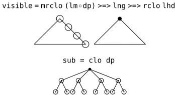
visible = mrclo (lm◦dp) >=> lng >=> rclo lhd
roles h d = [ r | Rule r p q cs←rules, p h, q d,
all ($ (h,d)) cs ]
The functionvisible(see Figure 3) returns the list of nodes connectable without violating the pro-jectivity requirement. These are reflexive transi-tive left heads (rclo lhd) of the left neighbour (lng) of the maximal transitive leftmost dependent
(mrclo (lm◦dp)). The functionroles, given two
nodes as arguments, selects roles which may label dependency connection between them. For each
rule Rule r p q csin the list of rules, it checks
whether the head and dependent nodes satisfy the predicates imposed on their categories (p and q, respectively), then verifies whether all constrains csapply to the head-dependent pair (($ (h,d)).
visible = mrclo (lm◦dp) >=> lng >=> rclo lhd
[image:8.612.99.273.623.718.2]sub = clo dp
Figure 3: Node functionsvisibleandsub
The set of constraints for our example include order constraints (left,right), agreement in gen-der (agrG), case (agrC), both case and gender
(agrCG), agreement between coordinated nouns
(agrCoord), and the constraint related to relative
close attachment (agrRel, see below).
right (h,d) = h < d left (h,d) = d < h
agrG (h,d) = (all masc∨all fem) [h,d] agrC (h,d) = (all nom∨all acc) [h,d] agrCG = agrC∧agrG
agrCoord (h,d) = or [ agrC (h’,d) | h’←hdBy Coord h ] agrRel (h,d) = or [ agrCG (h,d’) | d’←sub d, rel d’]
where sub = clo dp
The constraint agrCoord7 checks whether the nodeh has the headh’ linked by dependency of
type Coord and the agrCconstraint for h’ andd
evaluates toTrue;agrRelchecks whether the node dhas a transitive dependent d’ (i.e. subordinate node, function sub – see Figure 3) belonging to the categoryrelwhich agrees with the node hin case and gender. Finally, the list of grammar rules may be stated as:
rules = [ Rule Subj v (nominal∧nom) [agrG], Rule Cmpl v (nominal∧acc) [], Rule Coord n conj [right],
Rule CCmpl conj n [right,agrCoord], Rule Rel n v [agrRel],
Rule Mod n adj [agrCG] ]
Now, we will extend our grammar with con-straints on the cardinality of roles. Let’s intro-duce two more componenents to the grammar: the set of roles, which may appear at most once for each head (sgl) and the statements indicating roles which are obligatory for word categories (obl).
sgl :: [ Role ]
sgl = [ Subj, Cmpl, CCmpl, Rel ]
obl :: [ ((Node → Bool), [Role]) ] obl = [ (conj,[CCmpl]) ]
Singleness constraint will be defined as an in-stance of a more general mechanism: universal constraints – similar to constraints in rules but with global scope.
type UConstr = (Role,Node,Node) → Bool
singleness :: UConstr
singleness (r,h,d) =¬(r ∈ sgl∧ r ∈ dpr h)
uc :: [UConstr] uc = [singleness]
7We used the standard Haskell functionorhere, despite
its name is not intuitively fitting the context, because it does exactly what we need: it checks both whether the constraint
agrCreturnsTrueand whether there esistsh’for which the
Universal constraints will be checked before each dependency is added and will block the ad-dition in case any of them is violated. In order to incorporate them into our grammar we have to re-place the functionrolesused in the definition of
headsanddepsfunctions withroles’ defined as
follows:
roles’ h d = [ r | r←roles h d, all ($ (r,h,d)) uc ]
The functionroles’extendsrolesby addition-ally checking if all universal constraints (the list uc) apply to the connection being under consider-ation.
The obligatoriness constraint will be checked after completing the parse, in the pass function. The sat function looks for all roles which are obligatory for the argument node, as defined in the statements in theobllist, and verifies if all of them are present.
sat n = all (∈ dpr n) [ r | (p,rs)←obl, p n, r←rs ]
pass = all sat◦(pure ⊕ preds) (redefinition)
Here are some examples of the parser’s output:
> parse "widział Mari˛e i Jana"8
[ [ Step 4 Nma [(CCmpl,3)] [], Step 3 CONJ [(Conj,2)] [], Step 2 Nfa [(Cmpl,1)] [], Step 1 Vm [] [] ] ]
> parse "widział Mari˛e i Jan"9
[ ]
> parse "Jan widział ksi ˛a˙zk˛e któr ˛a czyta Maria"10
[ [ Step 6 Nfn [(Subj,5)] [],
Step 5 Vf [(Rel,3)] [(Cmpl,4)], Step 4 RELfa [] [],
Step 3 Nfa [(Cmpl,2)] [],
Step 2 Vm [] [(Subj,1)], Step 1 Nmn [] [] ] ]
> parse "Jan widział ksi ˛a˙zk˛e którego czyta Maria"11
[ ]
8he-saw Mary
+accand John+acc
9he-saw Mary+accand John+nom(agrCoordconstraint
vio-lated)
10John saw the-book+fem+accwhich+fem+accMary is-reading 11John saw the-book
+fem+accwhich+masc+accMary is-reading (agrRelconstraint violated)
6 Efficiency issues
As far as the efficiency issues are concerned, the most important problem appears to be the the number of alternative partial parses built, because partial parses with all possible combinations of le-gal connections (as well subsets thereof) are pro-duced during the analysis. This may result in un-acceptable analysis times for longer and highly ambiguous sentences.
This problem may be overcome by rejecting un-promising partial parses as soon as possible. One of the most obvious selection criteria is the for-est size (number of trees in a parse). The relevant parser modification accounts to introducing the se-lection function (for simplicity we use the fixed value of 4 for the forest size to avoid introducing extra parameters) and redefining thestepfunction appropriately:
select :: Parse → [Parse]
select p = if size p≤4 then [p] else []
step w = shift w >=> connect >=> select
The function sizewhich used to compute the number of trees in a parse may be defined as fol-lows:
size :: Parse -> Int size = foldr acc 0
where acc (Step _ _ h ds) n = n + 1 - length (h ++ ds)
7 All/first/best parse variants
The parser is designed to compute all possible parses. If, however, only the firstnparses are re-quested, then only these ones will be computed. Moreover, thanks to the lazy evaluation strategy, only those computations which are necessary to produce the firstnparses will be performed. Thus, no modifications are needed to turn the parser into a variant that searches only for the first or first nparses. It is enough to request only the firstn parses in the parser invocation. For example, the
parse1function defined below will compute only
the first parse.
parse1 = take 1◦parse
In order to modify the algorithm to al-ways select the best alternatives according to
someScoringFunction, instead of the first ones,
the parser may by further modified as follows:
someScoringFunction :: (Ord a) ⇒ Parse → a someScoringFunction = ...
sort :: [Parse] → [Parse]
sort = sortWith someScoringFunction
step w = shift w >=> connect >=> (sort◦select)
8 Conclusion
In the paper we have tried to show that a lazy func-tional language such as Haskell is a convenient framework not only for implementing dependency parsers but also for expressing dependency gram-mars directly as Haskell code. Even without intro-ducing any special notation, language constructs, or additional operators, Haskell itself allows to ex-press the grammar in compact, readable and math-ematically clean manner.
The borderline between the parser and the grammar is shifted compared to the traditional view, e.g. CFG/Earley. In the part, which we called the parser core, minimal assumptions are made about structural properties of the syntactic trees allowed (e.g. projective, nonprojective) and the nature of grammatical constraints which are formulated. In fact the only hard-coded require-ments are that the syntactic structure is represented in the form of a dependency tree and that the parse is built incrementally.
In order to turn the ideas presented above into a useful NLP tool for building grammars it would be obviously necessary to rewrite the code in more general, parametrizable form, abstracting over word category type (e.g. to allow structural tags), role type, parse filtering and ranking func-tions, the monad used to represent alternatives, al-lowing for representing some kinds of weights or ranks etc.
In fact, the work in exactly this direction is al-ready in advanced stage of development. In this paper it was reduced to the essential part (without parameterized data types, multi-parameter classes, monad transformers, and so on), which size allows to present it in full detail and with the complete source code in a conference paper.
References
Covington, M. A. (2001). A fundamental algo-rithm for dependency parsing. In In Proceed-ings of the 39th Annual ACM Southeast Confer-ence, pages 95–102.
de Kok, D. and Brouwer, H. (2009). Natural language processing for the working
program-mer. http://freecomputerbooks.com/books/
nlpwp.pdf. Accessed: 2016-11-22.
Eijck, J. V. (2005). Deductive parsing with sequentially indexed grammars. http://homepages.cwi.nl/~jve/papers/
05/sig/DPS.pdf. Accessed: 2016-11-22.
Erwig, M. (2001). Inductive graphs and functional graph algorithms. J. Functional Programming, 11(5):467–492.
Goodman, J. (1999). Semiring parsing. Computa-tional Linguistics, 25(4):573–605.
Hutton, G. and Meijer, E. (1998). Monadic parsing in haskell. J. Funct. Program., 8(4):437–444. Jones, S. P., editor (2002). Haskell 98
Lan-guage and Libraries: The Revised Report.
http://haskell.org/.
Koster, C. H. (1992). Affix grammars for natu-ral languages. In Alblas, H. and Melichar, B., editors, Attribute Grammars, Applications and
Systems, volume 545 ofLNCS, pages 469–484.
Springer-Verlag.
Kubler, S., McDonald, R., Nivre, J., and Hirst, G. (2009). Dependency Parsing. Morgan and Claypool Publishers.
Levy, R. and Pollard, C. (2001). Coordination and neutralization in hpsg. In Eynde, F. V., Hel-lan, L., and Beermann, D., editors,Proceedings of the 8th International Conference on
Head-Driven Phrase Structure Grammar, pages 221–
234. CSLI Publications.
Lipovaca, M. (2011). Learn You a Haskell for
Great Good!: A Beginner’s Guide. No Starch
Press, San Francisco, CA, USA, 1st edition. Ljunglöf, P. (2004). Functional chart parsing of
context-free grammars. Journal of Functional
Programming, 14(6):669–680.
Pereira, F. C. N. and Warren, D. H. D. (1980). Definite Clause Grammars for Language Analysis -A Survey of the Formalism and a Comparison with Augmented Transition Network. Artificial Intelligence, pages 231–278.
Ranta, A. (2011). Grammatical Framework:
Pro-gramming with Multilingual Grammars. CSLI
Publications, Stanford. ISBN-10: 1-57586-626-9 (Paper), 1-57586-627-7 (Cloth).
Yorgey, B. (2009). The typeclassopedia. The
Monad. Reader Issue 13, pages 17–66.
![Figure 1: The expression for the parse: [ Step 3 N [(Cmpl,2)] [], Step 2 V [] [(Subj,1)], Step 1 N [] [] ]](https://thumb-us.123doks.com/thumbv2/123dok_us/1489655.689114/5.612.334.509.230.488/figure-expression-parse-step-cmpl-step-subj-step.webp)