Annotating modals with GraphAnno, a configurable lightweight tool for multi level annotation

Annotating modals with GraphAnno, a configurable lightweight

tool for multi-level annotation

Volker Gast

Friedrich Schiller University Jena volker.gast@uni-jena.de

Lennart Bierkandt

Friedrich Schiller University Jena post@lennartbierkandt.de

Christoph Rzymski

Friedrich Schiller University Jena christoph.rzymski@uni-jena.de

1

Introduction

GraphAnno is a configurable tool for multi-level annotation which caters for the entire workflow from corpus import to data export and thus provides a suitable environment for the manual annotation of modals in their sentential contexts. Given its generic data model, it is particularly suitable for enriching existing corpora, e.g. by adding semantic annotations to syntactic ones. In this contribution, we present the functionalities of GraphAnno and make a concrete proposal for the treatment of modals in a corpus, with a focus on scope interactions. We have nothing to say about the specific categories to be annotated. Its generic design allows GraphAnno to be used with various annotation schemes, like those proposed by Hendrickx et al. (2012), Nissim et al. (2013) and Rubinstein et al. (2013). We will use generic category labels from theoretical linguistics for illustration purposes.

After providing some background information on the tool in Section 2 we show how GraphAnno deals with four major tasks of corpus-based projects, i.e., corpus import (Section 3), annotation (Section 4), searching (Section 5) and data export (Section 6).

2

Some background on GraphAnno

GraphAnno was originally designed as a lightweight prototype for a more powerful multi-level anno-tation tool, Atomic (cf. Druskat et al. 2014), in a project on multi-level annoanno-tation of cross-linguistic data.1 The focus was thus on functionality, rather than, for instance, performance with large data sets. The tool has been used in various corpus-based projects (e.g. Gast 2015), and it has proven a stable and user-friendly application, specifically for small-scale annotation projects. GraphAnno was therefore published in 2014, and will continue to be maintained.2

GraphAnno is so called because the corpus data is programme-internally represented, and also vi-sually displayed, as a graph, consisting of annotated nodes and edges. Given its generic data model, it can handle any type of graph structure, not only trees. Annotations can be restricted and controlled with dictionaries of attribute-value pairs.

The application requires Graphviz3_{and Ruby.}4 _{It handles dependencies on other libraries using the} RubyGems package manager. It is platform-independent, and an exe-file for easy use on a Windows system is available, bundling the required Ruby runtime environment. The tool has a browser-based interface. To get going, the user starts a ruby process (by double click or from a command line) and accesses the annotation projects by visiting the URL ‘http://localhost:4567’.

1

LinkType, sponsored by the German Science Foundation (DFG, grant GA-1288/5). Financial support from this institu-tion is gratefully acknowledged; see also http://www.linktype.iaa.uni-jena.de. 2 _{https://github.com/LBierkandt/graph-anno} 3

GraphAnno is operated via a command line at the bottom of the browser window. Annotations are created with one-letter commands such asn(create a node),g(groupe nodes into constituents),e(create an edge),d(delete nodes/edges) anda(annotation of attribute-value pairs; see below for examples). For navigation in the corpus and the choice of an annotation level, there are dropdown fields, and the tool comes with some key bindings giving access to its most important functionalities, e.g. for zooming and navigation. Some important functions are controlled with the function keys F6 (filter), F7 (search), F8 (configuration) and F9 (metadata). In the configurations window, users can, most importantly, define annotation levels and set some parameters concerning matters of visual representation (e.g. colours for annotation levels and highlighting), as well as define shortcuts and store search macros (cf. Section 5).

Unlike Atomic, which is part of the ANNIS-infrastructure,5 GraphAnno is intended to be ‘promis-cuous’, with interoperability being achieved via Python6and NLTK.7An important feature exhibited by GraphAnno which is not (yet) available for Atomic is the search and export functions (cf. Sects. 5 and 6). GraphAnno is thus designed for smaller projects and exploratory studies, as it allows users to analyse and inspect the data during the process of annotation. It is distinguished from other tools such as MMAX28 and Exmaralda9 by its focus on hierarchical multi-level annotation with (online) 2D-visualization, and from generic graph tools such as Cytospace10_{by its specifically linguistic functionalities.}

3

Corpus import

Corpora can be imported with the command import in the command line, which opens a dialogue window. They can either be loaded from a text file, or be pasted into a text field. For preprocessing, punkt segmenters for eleven languages are integrated and can be selected. A corpus format can also be specified using regular expressions. More richly annotated corpora, especially treebanks, can be imported via Python and NLTK. GraphAnno natively uses JSON-files for persistent storing. For the import of treebanks (e.g. the Penn Treebank)11 and of more specific resources like the the BioScope corpus12 (Vincze et al. 2008) converters are available. Being connected to the NLTK infrastructure already, an even closer integration is envisaged for the near future. Converted annotation projects are read into GraphAnno with theload-command, like any other project created with GraphAnno itself.

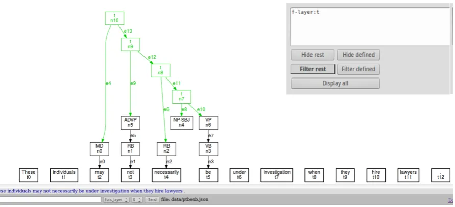
Figure 1 shows a structural representation of the sentence in (1), imported from the Penn Treebank. The sentence is displayed as a graph as well as in plain text at the bottom of the window.

(1) These individuals may not necessarily be under investigation when they hire lawyers.

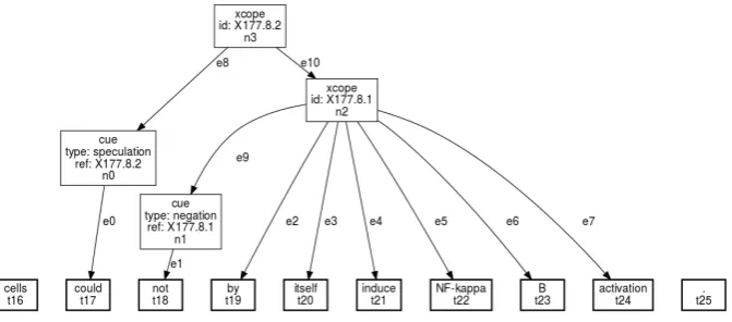
The sentence in (2), imported from the BioScope corpus, is shown in GraphAnno-format in Figure 2 (for reasons of space, only the part wih a modal is displayed).

(2) <sentence id="S177.8">

Oxidative stress obtained by the addition of H2O2 to the culture medium of J.Jhan or U937 cells

<xcope id="X177.8.2">

<cue type="speculation" ref="X177.8.2">could</cue> <xcope id="X177.8.1">

<cue type="negation" ref="X177.8.1">not</cue> by itself induce NF-kappa B activation

</xcope> </xcope>. </sentence>

While the BioScope corpus, as well as most annotation schemes for modals (e.g. Hendrickx et al. 2012; Nissim et al. 2013; Rubinstein et al. 2013), works at a single (structural) level of annotation, even though the annotations are (partly) semantic in nature, GraphAnno is a multi-level annotation tool and allows us

5

http://annis-tools.org/ 6 https://www.python.org/ 7 http://www.nltk.org 8 http://mmax2.sourceforge.net/

9

http://www.exmaralda.org/en 10 http://www.cytoscape.org/ 11 http://www.cis.upenn.edu/˜treebank/

Figure 1: A structurally annotated sentence in GraphAnno

to distinguish between a structural and a semantic layer. We argue that properties of semantic entities should be attributed to, i.e., annotated on, elements specifically representing meaning, not structure. Moreover, the advantage of multi-level annotation is that it allows us to add semantic annotations to existing structural ones – to enrich corpora, rather than annotating from scratch. We believe that by combining structural with semantic annotations, we can gain information that is potentially useful for machine learning. In what follows, we use syntactic structures as our point of departure and add manual annotations, which we consider a reasonable workflow for small-scale annotation projects.

4

Annotating modals manually

Having imported a corpus, it can be (further) annotated at a theoretically infinite number of levels. The levels are visually distinguished by colours, but they can also be separated by hiding specific levels, or filtering them out (cf. below). The structural level (‘s-layer’), as displayed in Figure 1, is by default blue.

4.1 Creating semantic structure

For a corpus-based study of modality, the annotation of scope relations is a central concern – for in-stance, because they interact systematically with the reading of a given modal (cf. von Fintel 2006 for a theoretical overview). For (1) above we can assume the simplified semantic representation shown in (3):

(3) MAY[NOT[NEC[ these individualsBEunder investigation . . . ]]]

As has been mentioned, GraphAnno allows for a free configuration of levels, including a free choice of names and colours, but it comes by default with two levels, the ‘s(tructural)-layer’ as represented in Fig-ure 1 above, and the ‘f(unctional)-layer’. We will use the functional layer for our semantic annotations. The annotation level can be selected from the dropdown field next to the command line, or in the com-mand line itself. Users can also choose to assign annotations to both levels by selecting the ‘fs-layer’. Note that annotations belonging to different levels can be searched together. Technically, they belong to the same graph. Assigning a given annotation to one level or another is thus often a theoretical decision and does not have any far-reaching practical consequences.

Scope relations holding between scope-bearing operators can be indicated by grouping the (denota-tions of the) constituents as shown in (3) on the semantic level (f-layer). In some but not all cases, the relevant structures are also represented syntactically, so that we can work on the fs-level. In a first step, we can create a node corresponding to the inner proposition ‘These individuals BEunder investigation . . . ’. For this purpose, we can assign the NP ‘these individuals’ and the VP ‘BEunder investigation . . . ’ to the f-layer (they belong to the s-layer already). Membership to a given level is stored as an attribute-value pair, with the name of the level as the attribute, and eithertorfas the value, but the level can be specified with a simple shortcut likef, too. Annotations can be assigned to several elements at the same time. For example, the nodesn2,n3andn4can be assigned to the semantic level as is shown in (4) (a

is the command for ‘annotate’).

(4) a n2 n3 n4 f

Figure 3: Hiding the structural level Having assigned the nodesn2,n3and

n4to the f-layer, we can create a parent node dominating them. Parent nodes are created with the command g (for ‘group’), followed by the identifiers of the nodes, and any attribute-value pairs. A node corresponding to the proposi-tion ‘these individualsBEunder investi-gation . . . ’ is created as is shown in (5) (the typet(Russell 1908) is assigned to the newly created node).

(5) g n13 n23 cat:t

We can now create successively higher-level nodes of typet, moving leftwards in the representation in (3) above. Inevitably in multi-level annotation, such annotations will lead to complex tree diagrams, and for users this may quickly become confusing. GraphAnno therefore allows users to hide or filter

Figure 4: Filtering the structural level

colours allow for a reasonably clear visual differentiation. When working on an annotation project, it is often more convenient to not just hide specific parts of a tree diagram, but to filter them out, i.e., to have GraphAnno display a new graph with only those portions of the graph that are currently relevant. It is important to note that the full structure of the graph is preserved, e.g. for search procedures; it is not represented visually, however.

Figure 4 shows the result of filtering out all those elements that are not represented at the semantic level. The small window in the top-right corner contains the filter criterion, heref-layer:t, and the graph shown in Figure 4 was generated be pressing ‘Filter rest’. Note that noden4, corresponding to the subject ‘these individuals’, appears to be dangling, but is actually linked to tokenst0andt1at the structural level.

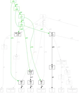
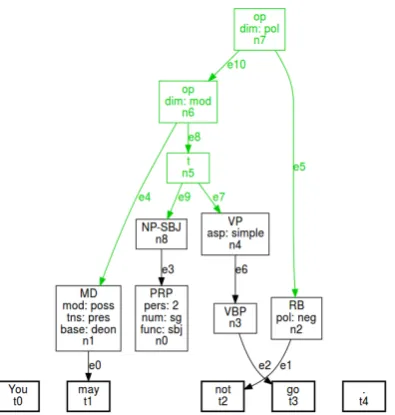
Figure 5: A deontic modal in the scope of negation In example (1), the order of

ele-ments mirrors their relative scope re-lations, and the graph is therefore rel-atively homogeneous in terms of its branching direction. An example of a modal being in the scope of negation (and thus leading to crossing edges) is shown in Figure 5. As the portion of the Penn Treebank that is accessible via NLTK does not contain an example of this type with may, we are using the made-up exampleYou may not go. Note that noden0, corresponding to the pro-nounyou, is not linked to its token, as the corresponding edge has not been as-signed to the f-layer.

4.2 Towards a richer annotation of modality

Such ‘element annotations’, which describe properties of constituents, can be restricted by dictionaries of attribute-value pairs. For example, we may want to annotate the tense and aspect categories of the main predicate in the scope of a modal (or negator), we might be interested in the person and number specifications of the subject, we may want to know what type of modality is expressed in each case, etc.

Figure 6: Element annotations As has been pointed out, element annotations

are created with thea-command, followed by the markable and attribute-value pairs. For example, if we want to indicate that a predicate is in the simple (rather than the progressive) aspect, we can specify this for noden5in Figure 6 as follows:

(6) a n5 asp:simple

Annotations concerning tense and aspect, the grammatical categories of the subject, etc. are po-tentially interesting for statistical analyses, as they may correlate with specific properties of modals (e.g. their readings) and specific scope configu-rations. Element annotations may be useful for other purposes as well. As we will see in Section 5, identifying specific scope configurations on the basis of purely structural information – as in Fig-ure 5 above – is possible but comes with certain disadvantages. It will therefore be beneficial to create annotations which represent sentence

se-mantic properties and configurations more directly. Ideally, such annotations should be created auto-matically from a certain point onwards. For a start, we need a manually annotated corpus. As has been mentioned, we can use any type of annotation scheme, e.g. the ones proposed by Hendrickx et al. (2012), Nissim et al. (2013) and Rubinstein et al. (2013), or the (much simpler) scheme used for the annotation of the BioScope corpus (Vincze et al. 2008). In the following discussion, we will not commit ourselves to any specific annotation scheme and use generic category labels. The focus is on the process of annotation, as well as the retrievability of the annotations (cf. Section 5).

One way of adding explicit scope information is by regarding the ‘higher’ nodes – thet-nodes in Figure 5 above – as ‘projections’ of the relevant operators, like thexcope-elements in the BioScope corpus (cf. Vincze et al. 2008). Let us assume that each scope-bearing operator projects a node of category ‘Op’, which is located at a position in the graph that corresponds to its scope domain. This projection is, obviously, located at the semantic level (though generative grammar has long assumed ‘LF-movement’ for syntax-semantic mismatches, regarding it as a syntactic operation). Let us furthermore assume that each ‘Op’-node comes with a specification for a ‘dimension’. For the study of modals, two dimensions are particularly interesting, i.e., ‘modality’ and ‘polarity’. Operator projections of scope-bearing elements will thus carry annotations of the type shown in (7).

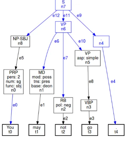
(7) a n7 dim:mod a n6 dim:pol

4.3 Representing ambiguities

Figure 7: Annotated operator projections Given that GraphAnno is a multi-level annotation

tool, representing ambiguities is no issue at all. As has been pointed out, the number of levels is the-oretically infinite. We can thus use different an-notation levels for alternative readings of a given sentence. Let us reconsider (2) above. The Bio-Scope annotators have analysed the sentence in such a way that the modal takes scope over the negation. While our knowledge of medicine is not sufficient to take a clear stance in this matter, the other reading, with the negator taking scope over the modal, actually seems more likely to us. Figure 8 shows the sentence with the two alterna-tive readings, represented at different levels (say, ‘sem1’ and ‘sem2’) and, hence, distinguished by colours (e8ande10are green,e9ande11blue) and, in the data structure, by different values for

the layer-parameters. (Note that in the graph shown in Figure 8, the identifiers linking a given scope domain to a cue have been removed, as scope dependencies are indicated with edges.)

Figure 8: Scope ambiguity in GraphAnno

Importantly, the alternative scope construals can be distinguished in the query (cf. Section 5), and users can search for specific scope configurations, as well as leaving relative scope relations unspecified.

5

Searching the corpus

5.1 The query language

GraphAnno has a powerful yet transparent query language. To search for tree fragments in the corpus, the search window is opened with F7. The user specifies a graph fragment by describing it in terms of attribute-value pairs associated with nodes, as well as links between nodes. The simplest case is a text search. For instance, one can search for the modalmaywithtext may. The hits are represented in red colour in the graph, as well as in the text line underneath.

(8) node cat:S|VP & !token

For more complex tree fragments, searches for nodes and edges can be combined. The declarationlink

is used to indicate that two nodes are linked by an edge (withedge), or a series of edges (withedge+). For single-edge links, we can also just useedgeinstead oflink...edge. To search for linked nodes, the nodes are described first and assigned a label. Node labels carry a@-prefix, as illustrated in (9), where two nodes are defined: @a(of category ‘VP’), and @b(of category ‘RB’, i.e., ‘adverbial’, in the Penn Treebank tagset). Finally, a statement is added saying that node@aand node@bare linked by an edge.

(9) node @a cat:VP node @b cat:RB edge @a@b

5.2 Retrieving (properties of) modals

The query language of GraphAnno offers more possibilities than pointed out above, but we will now focus on matters concerning modality. In Section 4, it was mentioned that we can identify scope config-urations on the basis of purely structural information, but that it is more convenient to have a more richly annotated corpus. Let us first consider how we can retrieve specific configurations without recurring to higher-level element annotations, i.e., from a structure of the type shown in Figure 5.

To find a modal in the scope ofnot, we have to search for a node of typet(defined in 10a) which dominates a modal (identified in 10b) while not dominating a negation. The first of these conditions can be expressed with the statement in (10c), referring back to the nodes defined in (10a) and (10b). The second condition can be implemented using acond-statement as shown in (10d). It specifies a condition saying that the set of nodes dominated by@pmust not contain a node with the annotation ‘token:not’.

(10) a. node @p cat:t

b. node @m cat:MD

c. link @p@m edge+

d. cond @p.nodes(’edge+’, ’token:not’).empty?

As for the more richly annotated structures, we have proposed to regard the top-level semantic nodes as projections of scope-bearing operators which are specified for a dimension, which in turn is represented as an attribute (with a value) on the daughter node, e.g. [dim:pol[pol:neg]]. Accordingly, we need three pieces of information in order to retrieve cooccurring scope-bearing operators. If we want to find a negator in the scope of a modal, we have to identify (i) a linked (ordered) pair of a modal operator projection and a polarity operator projection, (ii) a linked pair of a modal operator projection and a daughter node (with an attribute matching the dimensional value of its parent node), and (iii) a linked pair of a polarity projection node and a daughter node specified as a negator. Each such pair consists of a description of the two nodes in question and alink-statement. (11) shows how this query can be formulated in the GraphAnno query language.

(11) a. node @mop dim:mod # modal operator (projection) node @nop dim:pol # negation (projection)

edge @mop@nop # direct link from modal to negation op.

b. node @mod mod:poss # possibility modal

edge @mop@mod # direct link from modal proj. to modal

c. node @neg pol:neg # negation operator

edge @nop@neg # link from neg. op. (proj.) to negation

6

Data export

Figure 9: Displaying the result of (11) graphically Displaying search results

visu-ally, as illustrated in Figure 9, is a good way for manually in-specting corpora. What is more important in small- and mid-scale corpus studies, however, is the possibility of exporting data sets. GraphAnno has two export options. First, it al-lows users to export a subcorpus meeting the conditions specified in a query, i.e., a subset of sen-tences meeting the relevant con-ditions. For instance, with the type of query illustrated above, one could compile a subcor-pus containing only examples in which a modal is in the scope of

negation, or vice versa. The second type of data export creates a table for quantitative analysis.

Let us assume that we want to extract annotations for sentences in which modals and negation show scope interactions, and that we are interested in the following variables:

(12) a. the tense of the main predicate in the scope of the operator b. the aspect of the highest VP in the scope of the operator c. the modal base (in the sense of Kratzer 1977)13

d. the person and number of the subject

In a first step, we have to identify the nodes carrying the information in question, just like in a search query. We can use the statement in (11) for this purpose. In addition, we have to identify the nodes carrying the temporal and aspectual information, and the subject node. We also need to specify some intermediate nodes (such as the node standing for the inner proposition, t), as the data export (unlike a simple query) requires a coherent graph fragment. The following set of nodes or linked pairs, in combination with (11) above, will give us the desired results:

(13) node @prop cat:t # inner propositional node

link @mop@prop edge+ # link from modal op. to prop. node link @nop@prop edge+ # link from neg. operator to prop. node @vp cat:VP # VP-node

link @prop@vp edge # link from prop. to vp node @sbj cat:/.*-SBJ/ # subject node

link @prop@sbj edge # link from prop. node to subj

We can now define columns for the table to be exported withcol, followed by the column’s name and the annotation in question, in the format@node[’annotation’], as shown in (14).

(14) col mod @mod[’mod’] col base @mod[’base’] col tns @vp[’tns’] col asp @vp[’asp’] col sbj-pers @sbj[’pers’] col sbj-num @sbj[’num’]

13

7

Outlook

GraphAnno provides functionalities for a complete workflow from corpus import to data export and has been used in a number of annotation projects. With its command line interface, data input is fast, and its search and filter facilities allow users to inspect the (inevitably complex) data structures of multi-level annotation projects with reasonable ease. Even so, manual annotations are time-consuming, and automating them would represent a major step ahead in the corpus-based study of modals. It is our intention to use multi-level corpora that have been annotated with GraphAnno as an input to machine learning techniques in the near future, ultimately hoping to be able to automatically enrich existing corpus resources (like the BioScope corpus and the Penn Treebank) with additional layers of annotation.

References

Druskat, S., L. Bierkandt, V. Gast, C. Rzymski, and F. Zipser (2014). Atomic: An open-source software platform for multi-level corpus annotation. In J. Ruppert and G. Faaß (Eds.),Proceedings of the 12th Konferenz zur Verarbeitung natrlicher Sprache (KONVENS 2014), October 2014, pp. 228–234.

Gast, V. (2015). On the use of translation corpora in contrastive linguistics: A case study of impersonal-ization in english and german.Languages in Contrast 15(1), 4–33.

Hendrickx, I., A. Mendes, and S. Mencarelli (2012). Modality in text: A proposal for corpus annotation. In N. C. C. Chair), K. Choukri, T. Declerck, M. U. Doan, B. Maegaard, J. Mariani, A. Moreno, J. Odijk, and S. Piperidis (Eds.),Proceedings of the 8th International Conference on Language Resources and Evaluation (LREC ’12), Istanbul, Turkey. European Language Resources Association (ELRA).

Kratzer, A. (1977). What ‘must’ and ‘can’ must and can mean.Linguistics & Philosophy 1(3), 337–356.

Nissim, M., P. Pietrandrea, A. Sanso, and C. Mauri (2013). Cross-linguistic annotation of modality: A data-driven hierarchical model. In Proceedings of the 9th Joint ISO-ACL SIGSEM Workshop on Interoperable Semantic Annotation, Potsdam, pp. 7–14. Association for Computational Linguistics.

Rubinstein, A., H. Harner, E. Krawczyk, D. Simonson, G. Katz, and P. Portner (2013). Toward fine-grained annotation of modality in text. InProceedings of IWCS 2013 Workshop on Annotation of Modal Meanings in Natural Language (WAMM), Potsdam, Germany, pp. 38–46. Association for Com-putational Linguistics.

Russell, B. (1908). Mathematical logic as based on the theory of types. American Journal of Mathemat-ics 30, 222–262.

Vincze, V., G. Szarvas, R. Farkas, G. M´ora, and J. Csirik (2008). The BioScope corpus: Biomedical texts annotated for uncertainty, negation and their scopes. BMC Bioinformatics 9(S-11).