INTERNAL DOCUMENT 1 0
STORM SURGE PREDICTIONS BY THE gllASI UlilFOR STEADY WIND/PRESSURE FIELD METHOD
( 1 )
S. Ishiguro
1981
[This document should not be cited in a published bibliography, and is supplied for the use of the recipient only].
I N S T I T U T E OF O C E A N OCR A P H I C S C I E N C E S
%
00 W")INSTITUTE OF OCEANO'GRAPHIC SCIENCES
Wormley, Godalming, Surrey GU8 5UB
(042-879-4141)
(Director: Dr. A. S. Laughton)
Bidston Observatory, Birkenhead,
Merseyside L43 7RA (051-653-8633)
(Assistant Director: Dr. D. E. Cartwright)
Crossway, Taunton,
Somerset TA1 2DW (0823-86211)
INSTITUTE OF OCEANOGRAPHIC SCIENCES INTERNAL DOCUMENT 102
STORM SURGE PREDICTIONS BY THE QUASI UKSIFORM STEADY WIND/PRESSURE FIELD METHOD
( 1 )
S. Ishiguro 1981
CONTENTS
Abstract 3
1. introduction 4
2. Examples of quasi uniform steady wind/pressure field 6
2.1 Surge on 3rd January 1976 6
2.2 Surge on 1st February 1953 9
2.3 44 surge cases in 1898-1956 13
3. Formation of a quasi uniform steady wind/pressure 15 field and sampling
4. Surge predictions 18
4.1 Type-A prediction 19
4.2 Type-B prediction 28
5. Comparisons of the method with other methods 40
6. Further improvements of the method 43
6-1 Dynamic model 43
6.2 Sampling of input data 44
6.3 Statistical treatment of data 44
6.4 Determination of a field area 44
7. Conclusions 45
Acknowledgements 45
References 45
Appendix 1. Abbreviations and positions of coastal stations 47
2. Wind-pressure conversion 48
ABSTRACT
A new practical dynamic method for predictions of storm surges (positive and negative, coastal and offshore) in the North Sea has been developed with two variations: Type-A for daily-surges, and Type-B for an extreme surge occurring once in many (say 50) years.
The method has been based on the finding that a high surge in the sea is generated by a sustained wind/pressure field with an almost steady direction and a high wind speed. Such a field is represented by a simple field with a constant direction and magnitude over a finite duration. This is indicated by only three factors which characterize each storm case: wind direction, wind speed and duration. Factors for the pressure field are derived from the three factors.
A set of four water-level responses at each point in the North Sea is computed from the surge dynamic equations (or a model). Two of them are responses to two constant wind fields in orthogonal directions, and the other two are those for similar pressure fields. Each field is suddenly applied to the sea in a calm state. The responses are
expressed in a generalized form for an arbitrary intensity of the fields. Combining the above three factors and four responses by a simple additional computation, the maximum surge height at each point can be obtained for each specific surge case. Since the values of the responses are independent from each surge case, the set of responses can be used repeatedly.
For Type-A prediction, the three factors are obtained from forecast wind/pressure data. For Type-B prediction, only an extreme wind speed derived from a statistical analysis of observed wind data is available. Therefore, a technique to determine the maximum surge height at each point, only from the extreme wind speed, has been developed.
The simplified representation of a 'real' wind/pressure field by the three factors produces an error, other than errors associated with conventional dynamic surge computations. The error is reduced by the dynamic system of the sea which responds to an average value of exter-nal forces. Also the error tends to reduce when a surge is high, since a high surge is generated by an intense wind field which is closer to a simplified representation.
The above-mentioned simplification significantly benefits the practical surge prediction, particularly for Type-A: e.g. (1) surge data for the initial conditions of a dynamic computation is not
required; (2) the very small amount of input data needed from a weather forecaster can be transmitted even by telephone; (3) a simple addi-tional computation for each surge case can be carried out by a small computer in a short time; and (4) a minor running cost.
The method offers the prediction of the maximum surge height at each point in each surge case only, which the public is most interested in, and not the time-varying surge height.
1. INTRODUCTION
The North Sea has a history of disastrous coastal floods due to storm surges. Heavy traffic in the sea, including large vessels, requires more critical information of water level which is related to daily surge predictions. The recent increase in offshore constructions, due to the exploration of the North Sea for oil, requires extreme surge values in the long term, as well as daily surges.
Several surge prediction methods have been developed for the North Sea, starting with empirical-formula methods. The development of
dynamic-computation methods have made predictions of surges offshore possible which were previously difficult. The advance of the meteoro-logical forecasting, particularly with the introduction of a large-scale computer, has brought a good prospect of surge predictions by a combined operation of meteorological and surge models. However, these methods have not yet been used for routine surge-prediction services. One of the weak points of dynamics methods is their complexity which involves a large amount of data being transmitted and computed, and therefore
the facilities and running cost of a routine service becomes considerable. The method described in this paper is a dynamic method, and
pre-serves all beneficial parts of dynamic methods, such as a high capa-bility of simulation of a surge phenomenon in a sea having a complex topography and dynamic conditions. A significant simplification of the method from the operational aspect is derived from (1) the simplification of its input wind/pressure data, and (2) the limitation of its output to the maximum surge height only (not the time-varying surge height). (1) is based on the finding that a high surge is generated by a wind/ pressure field which is close to a uniform steady field. (2) satisfies most of the requirements of the public (the prediction of the timing of the occurrence of the maximum depends on the weather forecast) .
The method has two variations, Type-A for daily-surge predictions, and Type-B for a long-term extreme surge prediction. Both variations are based on the same principle. Predicted values by Type-A procedure can be evaluated from observed values which are easily available. Information on the accuracy of Type-A prediction can be extended to that of Type-B, which cannot be evaluated by the observational values in a short period.
2, EXAMPLES OF QUASI UNIFORM STEADY WIND/PRESSURE FIELD
The North Sea is sometimes covered by a sustained wind field having an almost steady direction with a high wind speed. Generally, the wind direction in the whole sea area varies slightly following the curvature of isobars, and also varies slightly due to the movement of the weather system. The wind speed varies with area and time, to a greater degree than the wind direction. The author calls this state a quasi uniform steady wind/pressure field, and finds that a high storm surge in the sea is generated by such a field.
Each of 17 storm-surge cases in the North Sea have been examined from this point of view, only two examples being shown in this chapter. Also, 44 storm-surge cases have been examined as a set of data which supports this theory.
In order to make the investigation objective, observational data (with minimum computational processes) have been used. Since historical observational surge data are limited to coastal ones, surge heights observed at coastal stations only are investigated with quasi uniform steady wind/pressure fields found in weather maps.
2.1 Surge on 3rd January 1976
Fig. 1 shows the wind/pressure field and surge in the North Sea on 3rd January 1976, sampled at 3-hourly intervals. The wind/pressure field is based on observational data analysed by Harding & Binding
(1978). The pressure field is shown by isobars (solid lines) with 2 mb intervals, and the wind field by equal-speed lines (dotted lines) with
10 kt intervals. The surge heights along the coast are shown by a bar graph*, taking surge height on the vertical axis, and the approximate position of each station on the horizontal axis with the abbreviation of the name of the station (see Appendix 1 for the full name and exact position).
When the depression centre is in the sea area (00 to 03 GMT), the surge heights are not great, with quite random polarities, since the surge is generated on a local scale by various wind directions in the sea area.
After the centre has moved out from the sea area (06 to 09 GMT) , the wind direction in the sea area has become more uniform, although the speed varies with area and time. The development of a high positive surge can be seen along the Netherlands and German coasts which are leeward of the wind field. A negative surge can also be seen around the south Norwegian coast which is windward of the field.
Throughout the rest of the period (12 to 21 GMT), the wind field is still sustained with a minor change of direction and the gradual decay of its speed. The surge height along the Netherlands and German coasts starts to decay, while that around Southend increases (due to a slight change of the wind direction).
s.
I
i
i
00 GMT 3 JAN 76
03
> 1 ! j j , '
11 1 ^
09
i l
B C 5 BG8S B fgiKBGa S B 8
SURGE HEIGHT (m)
2 iQ
1
ri\
MAXIMUM SURGE HEIQIT (m) OBSERVED ALONG THE COAST
w 5? P 0 o
s pT §
o o pT §
o > C"" 9
o n D* ^9
§ 8 w e* O m
Q m
0 ^
>c w 0 ^
w < M 2
M M
C4 O o
1 z
§ O
WK - 1
Bn;"'=rT2r=^&3=KKLr &:2!U3L&MrM&Lk;
BG
mm#oN
Zi&A^2033!%3B
i, i: (D
g P m >
c_,
g
UW.%.%u«u% ,'WCAkm-rLKma-W'A-'q—I -g
-5
(k \0 sj
, OBSERVED OFF-SHORE WIND
I
SPEED (kt) (X o
o
(BSERVED SURGE HEIOIT (m)
in O
Fig. 2 shows a set of diagrams which summarizes this surge case from the point of view of the formation of a quasi uniform steady wind/ pressure field.
The bar graph shows the surge along the North Sea coast. The envelope of this graph shows the maximum surge height during this surge case. The black part of the bar shows the surge height at the sampled time.
Surge height variations with time observed at a few representative coastal stations are shown in the top-right of Fig. 2. Since the surge observed offshore is not available, this is represented by a computed contour map for the sampled time (obtained from another dynamic method) and is shown in the centre of Fig. 2.
The wind/pressure field is represented by a synoptic weather map for a time nearest to the sampled time. The variations of represen-tative wind speed and direction observed at an offshore station are shown in the bottom-right of Fig. 2.
2.2 Surge on 1st February 1953
Fig. 3 is a similar diagram to Fig. 1, but for the surge around 1st February 1953. A set of diagrams to the left side of Fig. 3 shows the wind field on the sea surface. This wind field has been obtained from the observational data, by using the 'meteorological input-data processing system' (Ishiguro, 1979b). The pressure data is based on combined material supplied from the UK Meteorological Office and the Netherlands Meteorological Institute. The set of bar graphs to the right side of Fig. 3 shows the surge height along the North Sea coast. The data are based on Rossiter (1954) and the Netherlands Delta Committee
(1960), and are combined by the author.
A similar relationship between the wind/pressure field and surge generation to the previous example can be seen in this surge case. Namely, when the depression centre is in the sea area (12 GMT, 31st January), the surge heights are not great and their polarity is quite random. After the centre has moved out from the sea area (15 GMT), the development of the surge starts. The direction of the wind field-is very steady for about 24 hours. The dfield-istribution of the surge height along the coast, and their variation with time, clearly corres-pond to the direction of the wind field and the variation of wind speed with time, throughout the period. The surge is fully developed at 06 GMT 1st February, and the highest surge occurs on the Netherlands coast which is leeward of the wind field.
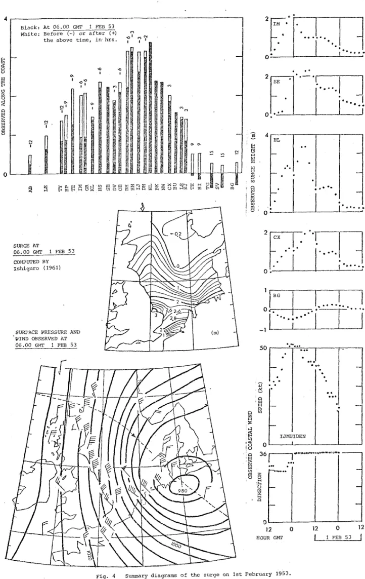
Fig. 4 is a diagram having the same format as Fig. 2, but for the February 1953 surge. The surge-height bar graph, offshore surge dia-gram, and synoptic weather map are sampled at 06 GMT 1st February. The offshore surge diagram was obtained by a full dynamic computation
(Ishiguro, 1961), and not by the method described in this paper.
10
g
- 1 — I — [ M 11 I I r r
12 GMT 31 JAN 53
T T - r n T T T n " T ~ T ~ r ~ i r
I i 11 I . i I i . I
.15
I
I I I I I I I
. . I
.18
0 GMT 1 FEB
I I I • ( I I ^
J_L
r m n - j
T T T
m
I I I I
— n n r
a a e s B s e e s ! ! s s a s s a s s s sasaa.s 8 s sI I I I I I I I I I I 11 I I I I 11 I I 11 I I _ l 1 L
;4-.
s W /
h ,
; t ; s \ ^ / / ^ / / / /
' / / / ' ' / / / <
^ X
/ . .. x T V /
X
y/z/z/^c^
Li
/ 3 r ^
/r
^ / / / / / (
cr c) T?,Lx
• v - i y /
SUR(3 HEIGHT (METRE PER DIVISION) OBSERVED ALONG 1HE COAST
LE
• TV ' HP .
^ IM ' G% ' KL
— HS
— - S E
DV OE
BH HH
— DH
— HL
BK
— m
— , c x
BU L5 EJ
-— HA
— H I
— TG
— S V
L BG
O o
J L
12
Black: At 06.00 GMT 1 FEB 53 white: Before (-) or after (+)
the above time, i n h r s . -gK
B M
ii
5 ag 8 Ba B 3 4
a K S B m
SUR(2 AT
06.00 GMl' 1 FEB 53
COMPUTED BY
Ishiguro C1961)
SURFACE PRESSURE AND
"KIND OBSERVED AT
06.00 GfT 1 FEB 53
i
1 §
•
SE
•
" . . .
1
c x
•
j B G
j L L - , , .
• •
1
IJMUIDEN
1 FEB 53 I
Fig. 4 Summary diagrams of the suroe on
12 0
HOUR @4T
13
2.3 44 surge cases in 1898-1956
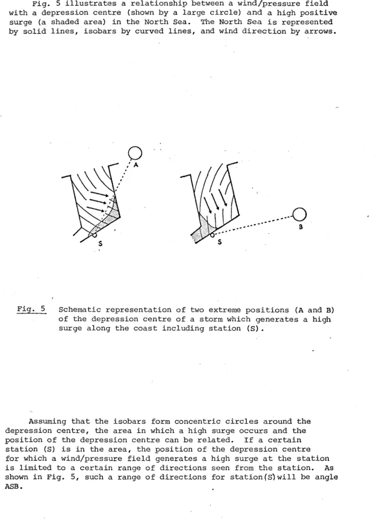
Fig. 5 illustrates a relationship between a wind/pressure field with a depression centre (shown by a large circle) and a high positive surge (a shaded area) in the North Sea. The North Sea is represented by solid lines, isobars by curved lines, and wind direction by arrows.
\ \ y
o
Fig. 5 Schematic representation of two extreme positions (A and B)
of the depression centre of a storm which generates a high surge along the coast including station (S).
Assuming that the isobars form concentric circles around the depression centre, the area in which a high surge occurs and the position of the depression centre can be related. If a certain station (S) is in the area, the position of the depression centre for which a wind/pressure field generates a high surge at the station is limited to a certain range of directions seen from the station. As
shown in Fig. 5 , such a range of directions for stationfs) will be angle
14
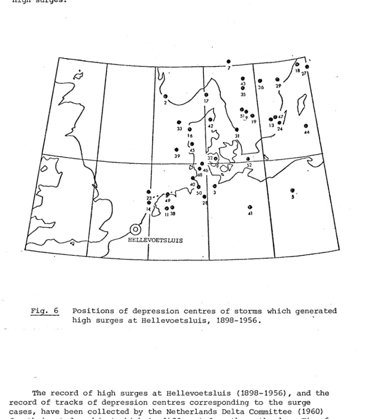
Fig. 6 shows evidence of this theory. Each dot (with case reference number) shows the position of the depression centre o f a storm at the time when a surge greater than 150 cm was recorded at Hellevoetsluis. This shows that most of these 44 storms formed quasi uniform steady wind/ pressure fields as defined in this paper, and that such fields generate high surges.
(J
HELLEVOETSLUIS
Fig. 6 Positions of depression centres of storms which generated high surges at Hellevoetsluis, 1898-1956.
15
3. FORMATION OF A QUASI UNIFORM STEADY WIND/PRESSURE FIELD,AND SAMPLING As shown by the examples in the previous chapter, a high surge in a semi-closed sea is generated by a quasi uniform steady wind/pressure field (defined on page 5). Fig. 7 illustrates some possible variations of positions of a storm system relative to the sea. In all the cases, except for such a field would be formed, if the size of the storm system is large compared with the sea, and if the system changes slowly, or moves slowly. By interpreting the generation of a high surge in this way, the high surge and storm system can be related more simply and clearly.
©
,•,
©
. . V ©
-\
- - •
///
/
(©
© "
/
•U--
xT,"-;:-Fig. 7 Variation of positions of a storm system relative to. a semi-closed sea (thick lines). A circle shows a depression centre, curved lines show isobars, and an arrow shows a wind direction.
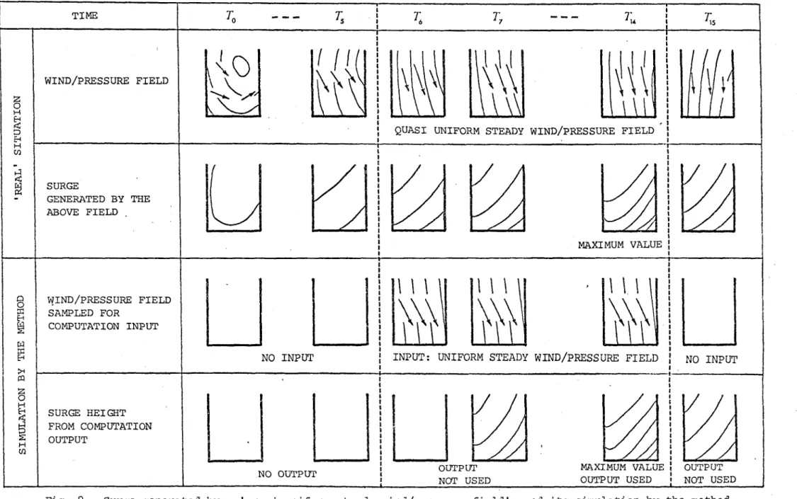
Fig. 8 illustrates the development of a quasi uniform steady wind/ pressure field (1st row), and the generation of a high surge (2nd row) both in a 'real' situation. This also illustrates a sampled wind/ pressure field for the computation in the method (3rd row), and the computed surge (4th row). In the real wind/pressure field, a duration, in which the wind direction is almost steady, and at the same time, the wind speed is high is sampled as a quasi uniform steady wind/pressure
TIME 71 r .
§
Hi
E - i
H
W
<
WIND/PRESSURE FIELD
SURGE
GENERATED BY THE ABOVE FIELD
V
7:
1
QUASI UNIFORM STEADY WIND/PRESSURE FIELD
MAXIMUM VALUE
77.
1 1
§
I
CQ
8
gS
H
C/2
WIND/PRESSURE FIELD SAMPLED FOR
COMPUTATION INPUT
1 1 1
\\\
1
\\\
1
!
\\\
L I
NO INPUT INPUT: UNIFORM STEADY WIND/PRESSURE FIELD NO INPUT
SURGE HEIGHT FROM COMPUTATION OUTPUT
NO OUTPUT OUTPUT
NOT USED
MAXIMUM VALUE OUTPUT USED
OUTPUT NOT USED
Fig. 8 Surge generated by a 'quasi uniform steady wind/pressure field', and its simulation by the method.
Thick lines: sea area (the topography in the model is not simplified). Thin lines in the 1st and 3rd rows; isobars. Thin lines in the 2nd and 4th rows; surge contours. Arrows; wind vectors.
17
WIND DIRECTION
WIND SPEED
WIND-GENERATED SURGE (HEIGHT)
" — — -••1— ••• —
r 1
l\ _ 1
, 1
-y t\
* DURATION • TIME
Fig. 9 'Real' wind and wind-generated surge (solid lines); and a simulated wind and wind-generated surge (dotted lines). A duration in which the wind direction is almost steady, and at the same time, the wind speed is high is selected as a 'quasi uniform steady wind/pressure field*. Wind direction and speed averaged over the duration is used for a simulated wind field in the method. Pressure field and pressure-generated surge are treated in a similar way.
Fig. 9 illustrates the same relationships between the fields and surge as in Fig. 8, but the time variations of the wind direction,
wind speed and wind-generated surge at a point in the sea. The pressure direction, pressure gradient and pressure-generated surge have similar relationships.
The representation of a quasi uniform steady wind/pressure field, which in fact varies with time and space to some degree, by a constant field produces an error. However, the error reduces in the maximum value of a high surge, since the dynamic system of the sea generally responds to an average value of the time-and-space varying external forces.
As a wind/pressure field dealt with in the method is constant, this can be represented by only three factors: wind direction, wind speed and duration; or pressure-direction, pressure gradient and duration (the same as the duration of the wind field).
18
4. SURGE PREDICTIONS
The frequency of occurrence of surge heights exceeding a certain level at a point in the sea area generally reduces, if the reference level is increased. If the frequency is fixed, the reference level varies from point to point considerably. Since the author is interested in surges on the scale of the whole North Sea, it is convenient to
classify surges into two categories by referring to their frequency of occurrence, rather than surge heights:
Daily surges
Surges occurring quite frequently in a season; and Long-term extreme surge
Surge occurring only once in many (say 50) years. Then, two types of surge prediction are considered in the method:
Type-A Daily surge prediction; and
Type-B Long-term extreme surge prediction.
Both the types of prediction are based on the finding that a high surge (positive and negative) in a semi-closed sea (like the North Sea) is generated by a quasi uniform steady wind/pressure field (defined and confirmed in chapter 2) . Such a field can be represented by a uniform steady field and indicated by only three factors (chapter 3).
A set of four water-level responses at each point in the North Sea is computed from the surge dynamic equation (or a model) , Two of them are responses to two uniform steady wind fields applied in orthogonal directions, and the other two are those for similar pressure fields. Each field is suddenly applied to the sea in a calm state. The responses are expressed in a generalized form for an arbitrary intensity of the fields.
Combining the above three factors and four responses, the maximum surge height at each point can be obtained for each specific surge
case. Since the values of the responses are independent from each surge case, the set of responses can be used repeatedly.
For Type-A prediction, the three factors are obtained from forecast wind/pressure data. For Type-B prediction, only an extreme wind speed is available. Therefore, a technique to determine the maximum surge height, only from the extreme wind speed, has been developed.
The method (both Type-A and Type-B) offers the prediction of the maximum surge height at each point in each surge case, and not the time-varying height.
19
4.1 Type-A prediction
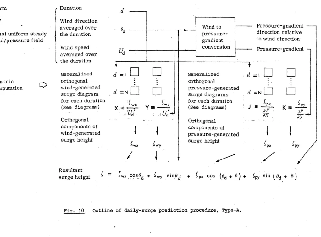
Fig. 10 shows an outline of Type-A prediction procedure.
Before the operation, sets of water-level responses, X, Y, J, K, have to be computed from the surge dynamic equations (or model). X and Y are responses to two uniform wind fields in the x and y direc-tions respectively. J and K are responses to two uniform pressure fields in the x and y directions respectively. Each field is suddenly applied to the sea in a calm state, and the value of response at the end of duration of d is obtained. Each value is given in a generalized form so that this can be used with an arbitrary wind speed or pressure gradient. Since the values depend on duration d, different sets of X, Y, J, K are required for different d's in principle. In practice, about 10 sets with logarithmic intervals of d have been found to be sufficient. Examples of X, Y, J, K indicated by diagrams are shown in Figs. 11 and 12, although their numerical sets are also available.
A surge prediction starts with finding a quasi uniform steady wind/pressure field from a forecast wind/pressure data, and indicating
it by the three factors: d, 8^ and From Uj and the pressure
gradient, 9p/8x or dp/dy, and its direction (relative to the wind direction) 0, can be determined, by assuming a certain relationship between a wind field and a pressure field (see Appendix 2) .
Next, an appropriate set of X, Y, J, K is selected by d. Then
Cwx ^wy Fig. 10) are determined by applying to the selected
X and Y; and and Spy are determined by applying 3p/3x or 3p/3y to
the selected J and K. Finally the resultant surge height ^ is deter-mined by the last equation in Fig. 10.
Table 1 (pages 24 and 25) shows an example of a programme for the operation shown in Fig. 10. The programme has been written in a basic language so that this can be applied to a small table-top computer. This example contains the values of X, Y, J, K for 30 coastal stations along the North Sea coast. The same programme, but containing 60 off-shore stations in the North Sea, is also readily available.
Figs. 13 and 14 show examples of computed and observed surge heights along the North Sea coast (see the footnote on page 5, for the format). Although computed data are available for both coastal and offshore stations, coastal data only are compared, because obser-vational data offshore are not available. In each figure, the
envelopes of the computed and observed bar graphs should be compared. Note, stations in the two types of graph are not exactly the same.
20
Fig. 14 shows the 3rd January 1976 surge. The wind/pressure field for this surge case was simulated by two constant fields, since the wind direction was changed considerably without decaying the wind speed. The values of the two fields are shown in the top-left of the upper diagram. The computed surge heights derived from the first and second fields are shown by black bars and white bars respectively. In the lower diagram, a surge height observed at the sampled time is shown by a black bar. The maximum surge height occurring at each station during this surge case is shown by a white bar.
Storm
Quasi uniform steady
wind/pressure field
Dynamic
computation
oDuration
Wind direction
averaged over
the duration
Wind speed
averaged over
the duration
Generalized
orthogonal
wind-generated
surge diagram
for each duration
(See diagrams)
Orthogonal
components of
wind-generated
surge height
Resultant
surge height
= , • •
d =1
^ = N [ ]
V6
•
X = ' wx
$
I
I
>wy
/ 1
Wind to
p r e s s u r e
-gradient
conversion
Generalized orthogonal pressure-generated surge diagrams for each duration (See diagrams) Orthogonal components of pressure-generated surge heightPressure-gradient
direction relative
to wind direction
Pressuregradient
-1
d
• •
d = N [ i ] n
I px
if
'px
K 5
i py
ay
1
I
i -
^wx cosOj +
s i n g j
+ (px cos \d^ + A) + ^py sin ^0^ + /5)
Fig. 10 Outline of daily-surge prediction procedure. Type-A.
V.'ND W ND
\
Fig. 11 Example of the generalized water-level responses, X and Y, to
the orthogonal uniform wind fields which is suddenly applied to the North Sea in a calm state. Line value; x 0.01 cm/(m/s)*
PRESSURE PRESSURE
Table 1 Programme for Type-A prediction.
2 4
In Fig. 10
d
u.
^wy /^d ( /aP
^py ^ ay a
T Duration
D Wind direction averaged over the duration
U wind speed averaged over the duration
X Generalized water-level response to a uniform wind field in x direction
Y y d i r e c t i o n
J Generalized water-level response to a uniform
pressure field in x direction
K y direction
A Angle between wind direction and isobar
B Angle between wind direction & pressure-gradient direction W Wind-generated surge height p Pressure-generated surge height R Resultant surge height
I Station number
a is not shown in i Fig. 10.
hours degrees m/s
cm/ (m/s) ^ cm/ (m/s):
cm/(mb/100 km) cm/(mb/100 km) degrees degrees cm cm cm
Programmes for coastal and offshore stations are the same, but they are recorded on separate parts of a cassette tape
for convenience.
As data (X, Y, J, K) in the programme have specific values for each station and for each duration, they are also recorded on a separate section of the tape.
The programme shown on the next page is an example of a particular section of the tape containing the specific values for 30 coastal stations for a duration.
To use,
(1) Select the part required 'coastal' or 'offshore'; (2) Select the section for the required duration T; and (3) Specify wind speed U and wind direction D by using
the computer keyboard.
2 5
Programme for Type-A prediction (Table 1, continued) 10 LET T=20
12 LET U= 14 LET D= 30 OPEN 2,4 35 CMD 2
38 PRIHT#2.. "HHP COflSTflL SURGE"
39 PRINT#2, "T="; T.: " (HR) " j " U="U; " (M/S)" " D="D; " (DEG) " 40 PRINT#2,
42 PRINT^2.. "ST", "W<CM)", "PO'JV", "R<CM>" 45 CLOSE 2
50 FOR 1=1 TO 30
51 DATA —5.'—3. 7.'—ii. i:, 1.3.' —7. 4, —1. fc', —2. S, iil. 2^' —9.2.'—1.6, —3.4,3.2 52 I'ATA —Iw, U. 0, —4. 0.' y. 6, — 11. y, 7, —y. 6, y. 6 — 1 4 . 5, —4.5,4.1 53 DATA -14,23.3,-4.5,4.7, -14.3,23.3,-3.3,5.6, -14.2,31,-3.3,6 54 DATA -9,30.5,-1.3,5.1, -5.5,23,-1.5,4.6, -4.2,23,-1.5,4.2 55 DATA u, 0, —. 4, 4. 3, U. 0, y U ,—.2,4.5, 0. 0, 30, —. y, 4. 7 5b DATA y. u, 30, —. 1,5, y. 0,2z'. 5,
—-57 DATA 4,19.3,.5,5.2, 6.3,IS.3,. 58 DATA 30.5,15.8,2.5,4.8, 35,13. 59 DATA 25,6,3.2,2.3, 16,-7.3,2.7
60 DATA 7.2,-11.5,1.9,1, 4.3,-12.5,1.2,.2, 3.2,-10.5,1.4,-1.5 200 READ X,V,J,K
210 LET X=X*(U/10)f2 212 LET V=V»i(U/10> r2
214 LET J=J*(.653*U12+14.37*U+f2.2)*.008192 216 LET K=K$(.653W12+14.37*U+12.2)*.008192 220 LET A=22
222 LET E=90-fl 224 LET C=D+112
230 LET 1#X.^:C0S< C*ir/180) + V$SIN(G*:;r/180) 232 LET P=J*COS((C-B)*#/180)+K*SIN((C-B)W/180) 234 LET R=W+P
240 W=INT(W+.5) 242 LET P=INT(P+.5) 244 LET R=INT(R+.5) 300 OPEN 3,4
302 CMD 3
304 PRINT#3,I,W,P,R 306 CLOSE 3
313 NEXT I
3,5.2, -.3,21.8,.1,5.2 5,5.2, 14.5,16,1.5,5
26
4 m
- 1
T=18 0=30 D=j30
1 FEB 1953 06.00 GMT
OBSERVED
s 8 a g K M S H HI X U (Qi^H O m
Pig. 13 Con^arison of surge height computed by Type-A prediction procedure, with surge height observed along the North Sea coast, at 06.00 OfT,
27
m
T=16 T^ZO
U=32 U=28 D=290 D=340
x+c x+c
C O M P U T E D
3 JAN 1976
I 12.00 GMT
Eh K M ( 0 33
o > m hqh K m
2 8
4.2 Type-B prediction
A long-term extreme surge can be predicted in the same way as Type-A prediction procedure, if the predicted long-term extreme values of a wind direction, wind speed and duration are available. In prac-tice, however, only a once-in-50 year extreme wind speed is available for the North Sea area, without other information. Type-B prediction procedure has been developed for this situation..
Fig. 15 Once-in-50 year extreme wind' speed over the North Sea area (Shellard, 1974).
29
S
I
g
5
1,0
. 0.5
—
i9-:l~
r-zt"
a :
F„(t)
--f i-;
——-r
-t-.p.
j — —
rzt::
: #
—4--I":
EMPIRICAL DATA (SHELLARD 1975) FORMULA (ISHIGURO 1980)
-l
2 0 40
Duration, (t) hours
6 0 80
Fig. 16 Reduction factors for the once-in-50 year extreme wind (hourly-mean speed) , when it is used for a duration longer than one hour.
The author has found a single formula;
F^(t) = 0.79 - 0.00394t + 0.25e"°'^^^ (t in hours)
which covers all Shellard's reduction factors. The upper dotted line in Fig. 16 shows the values of the reduction factor with hourly
30
According to the above information, the predicted once-in-50 year extreme wind speed reduces following the reduction factor of (t) which is a function of time (duration) . On the other hand, a surge generated by a suddenly applied uniform wind field increases (positively or nega-tively) with time. Therefore, a surge, generated by a suddenly applied uniform wind field having a predicted wind speed with a certain duration, depends on the duration. Generally, the surge height becomes maximum
(positive or negative) at a certain duration. Fig. 17a illustrates these relationships.
WIND-SPEED REDUCTION FACTOR, (F„(t))»
WIND-SPEED REDUCTION
WATER-LEVEL RESPONSE TO A SUDDENLY APPLIED UNIFORM WIND FIELD
WATER-LEVEL RESPONSE TO A SUDDENLY APPLIED UNIFORM PRESSURE FIELD
VARIATION OF WIND-GENERATED SURGE HEIGHT WITH THE DURATION OF THE FIELD
max
VARIATION OF PRESSURE-GENERATED SURGE HEIGHT WITH.THE DURATION OF THE FIELD
TIME. TIME
(a) (b)
Fig. 17 Relationships between the wind-speed reduction factor,
water-'level response to a suddenly applied uniform field, and a surge height variation with the duration of the field. (a) Wind-generated surge. (b) Pressure-generated surge.
Since the information of a once-in-50 year pressure field is not available, this has to be estimated from the predicted once-in-50 year extreme wind field, assuming a certain relationship between the two fields. For example, the pressure gradient and its direction can be estimated from the wind speed and direction, although the absolute values of pressure field cannot be estimated from the wind field data. A pressure gradient determined in this way reduces following the reduc-tion factor of F^(t) which is again a funcreduc-tion of time. A surge
generated by a suddenly applied uniform pressure field increases
(positively or negatively) with time, but with a different characteris-tic from the wind-generated surge. A surge generated by a suddenly applied uniform pressure field having an estimated pressure gradient becomes maximum (positive or negative) at a certain duration. Fig. 17b illustrates these relationships.
31
Fig. 18 shows an outline of Type-B prediction procedure, which determines the maximum value of the resultant surge practically. This starts with three types of factors:
(1) Predicted once-in-50 year extreme wind speed; (2) Water-level responses; and
(3) wind-speed reduction formula.
(2) has been obtained from the surge dynamic equations (or model) , with the conditions that uniform wind fields in orthogonal directions are suddenly applied to the sea in a calm state. (2) is combined with
(3). Then the maximum value of the combined factor for each point is determined numerically by varying the duration (t) . X and Y in Fig. 18 indicates the maximum values of wind-generated surges in the x and y directions respectively obtained in this way. Fig. 19 is an example of a set of diagrams showing the values of X and Y for the North Sea. J and K in Fig. 18 indicate the maximum values of pressure-generated
surges in the x and y directions respectively, obtained in the same way. Fig. 20 is an example of these values.
By applying a predicted once-in-50 year extreme wind speed (hourly-mean value) Uj to factors X and Y, the maximum surge heights at each point generated by the wind fields in the x and y direction, and are obtained. Similarly, by applying a once-in-50 year extreme pressure gradient, 3p/9x or 9p/8y, which is estimated from Uj, to factors J and K, the maximum surges at each point generated by pressure field in the x and y directions respectively, Zpx ^py' determined.
The resultant surge ^ is given by the penultimate formula in Fig. 18, which is a function of Cwx' ^wy ^px' ^py' ® 6^. By specifying the values of the first four parameters from the above information, and by
specifying the value of 3 which is the direction of the pressure field relative to the wind direction, the formula becomes the function of wind direction 6^ only. Therefore, by choosing the value of 9^ so that ? becomes maximum, the maximum surge height Cmax ^rid the wind direction
®w max which generates such a surge can be determined. The pressure-field data can be derived from the wind-field data, by using a certain relation-ship (see Appendix 2).
The determination of ^max ®w max the last equation in Fig. 18 can be carried out either by (a) a totally numerical computation (varying the value of 8^) , or (b) by using an analytical formula which determines the maximum value directly. The author uses (b) with a minor
simplifi-cation. The formula has been described in a separate paper (Ishiguro, 1976) Table 2 is an example of the programme for the operation shown in
Fig. 18, which includes the analytical formula in (b) , but excludes the surge-dynamic equations from which the values of X, Y, J, K have been derived. The programme in Table 2 has been written again in a basic language so that this can be processed by a small table-top computer. The same programme can be used for both coastal and offshore stations, although the example shown in Table 2 contains the values of X, Y, J, K and E (see page 35) for each of 30 coastal stations along the North Sea coast. Another set of programmes containing 60 offshore stations is also available.
Once-in-50 year
extreme
hourly-mean wind speed
Dynamic
computation
Sheila r d
-Ishiguro
formula
Generalized
orthogonal
wind responses
Wind-speed
averaging factor
(Function of time)
Product of the
above two
functions
^ wx(^ ) ^wv(0
1 I
FJ')
u r f M - ^
Maximum of the
above product
(See diagrams)
Orthogonal
components of
maximum
wind-generated surge
Resultant surge
(Function of
wind direction)
Maximum
resultant surge
I
— ^ W
Ui
wx wy
X X
^ — ^wx +
^max — ^ ( ^wmox )
Wind to
p r e s s u r e
-gradient
conversion
Pressure-gradient
direction relative .
to wind direction
Pressure gradient
Generalized
orthogonal
p r e s s u r e responses
Pressure
averaging factor
(Function of time)
Product of the
above two
functions
^px(0 ^py ( 0 A
I
Maximum of the
above product
(See diagrams)
Orthogonal
components of
maximum p r e s s u r e
-generated surge
^ px(0
I
J =
^ px
I F "
K =
py
^7
px
^wy + ^px: COS {9y,+ji) + tpy s i n (^vv+^j
Wind direction
O^^nax is chosen
SO that {,
becomes maximum.
0+ 0
J
W ND WIND
Fig. 19 Example of the generalized water-level responses, X and Y, to
PRESSURE PRESSURE
Table 2 Programme for Type-B prediction.
35
In Fig. 18
^wy/ U]
*px/a% 9y a wn € A
u
X Y J K A B D E L R IHourly-mean extreme wind speed Generalized water-level
response to a uniform
pressure field in x direction y direction Generalized water-level
response to a uniform wind field in x direction '
y direction
Angle between wind direction and isobar
Angle between wind direction and pressure-gradient direction Angle between wind direction and model grid axis
Wind direction
Direction of model grid Angle introduced for quadratic selection
rnximum resultant surge height Station number m/s cm/(m/s)^ cm/(m/s)^ cm/(mb/100 km) cm/(mb/100 km) degrees degrees degrees degrees degrees degrees cm
a,9y^f^,e and . A are not shown in Fig. 18
Programme for coastal and offshore stations are the same, but they are recorded on separate parts of a cassette tape for convenience.
An example of the programme for 30 coastal stations is shown on the next page. Equations in Lines 123 to 428 have been derived from the theory described in a separate paper
(Ishiguro, 1976).
To use, select an appropriate part first, then specify an extreme hourly-mean wind speed by using the computer keyboard. If the output of the programme indicates 'CHECK DATA', the values of a set of data (X, Y, J, K) in the line at which the computation stopped might have an illogical combination, and this should be cleared.
Programme for Type-B prediction (Table 2, continued)
0 REM "SPECIFY HOURLY-MEAN EXTREME WIND SPEED IN (M/S)" 2 LET U=
4 OPEN 2,4
6 CMD 2 '
8 PRINT#2,"BBP COASTAL SURGE"
10 PR I NT#2, "HOURLY-MEAN EXTREME WIND SPEED U=".iU.: "(M/S)' 12 PRIHT#2,
14 PRINT#2,"ST",' 16 CLOSE 2
20 FOR 1=1 TO 30
R(CM)","D(DEG)"
24
DATA
DATA DATA 28 DATA 30 DATA 32 DATA
34 DATA
3b DATA 38 DATA 40 DATA 44 DATA 46 DATA 48 DATA 50 DATA 52 DATA
-17.4,-2.1,-2.6,2.1,27. -17.5,16,-3.6,3.1,26.8, -15,16, -3, 3.2, 26. 2, -12.S,19,-2.5,4.3,25, -11.4,21.8,-2.9,4.2,24. -10,18,0.0,3.2,23.6, —3. 3, 16, 1.6, y. 6, 22, -2.8,18.5,1.2,4,21.4, -2,14.5,1.4,4.3,20.7, 4.8,11.8,1.7,4.4,20.3, 10.4,10.1,1.5,4.5,19.1,
i , -10.5,2.5,-2.8,2.7,2 -19.2,20.6,-3.6,3.2,27 -14,19,-3.2,3.8,25.8
-12.6,20,-2.2,4.8,24.6 !, —7, 19, — 1. 6, 3. y, 23. 1
-11,18,0.0,3.0,23.9 -2.9,18.5,1.2,3.9,21.5
-2.5,18.5,1.3,4.2,21 —.1,12.9,1.4,4.3,20. 6
5.8,10.5,1.6,4.2,20.3 24,10.3,2.2,4.7,17.5
1 y. 4,6. j, 2.3,4.1,1 y
8.7,-7.4,1.8,2.6,18 ' 18.5 24,9,2.2,4.5,17.6,
14. y, 1. 5,2. 6,3. 6, 18.1,
6.2,-9,2.7,2.2,17, 5,-10,1.9,1.2 4. 2, —9. 6,1. 4,. 5,20, 3, —9,1. 3, - . 6 100 READ X,V,J,K,E
111 LET X=X*(U/10)i2 112 LET Y=Y*(U/1S)12
113 LET .J=J* ( . 653$U f2+14. 37*U+12.2 > *. 008192 114 LET K=K*(.653*Ut2+14.37*U+12.2)*.008192 119 LET A=22
120 LET E=S0-fl
121 LET C=COS(B*ir/180)
122 LET 8=SIN<B5tsir/180>
123 LET M=X12+(J*C+K*S)12+2*XM*(J*C+K*S)
124 LET N=Yf2+(K*C-J*S)t2+2$Y*C*(K*C-J*S)
125 LET 0=2*(X*Y+(JK+K*S)*(K*C-J*S)+X*C*(K*C-J*S)+V*C*(J*C+K*S))
127 LET L=S.5#(180/IT*ATN<ABS';Q/(M-H>)>) 200 IF SGN(Q>=1 THEN 202
201 GOTO 300
202 IF SGN(M-N)=1 THEN 210 203 GOTO 250
210 IF AES< :x)' ::=AES<Y > AND SGN<; o = i AND SGN( V >=1 THEN 400 212 IF ABS< X.V :=PES';v ) AND SGNC; 4)=-l AND SGNC Y THEN 404 214 IF ABS'; >=ABS(Y ) AND S G N C 0 = - ! AND SGNC Y >=-1 THEN 404 216 IF ABS( X): >=AES'::V ) AND S G N C «:)=-i ANDS :ON(Y = 1 THEN 404 IF AES' >=ABS<Y :> AND SGN';: o = i AND SGNC V ) = 1 THEN 400 IF AES< :x): >=ABS(Y ) AND S G N C >o=i AND SGNC V — 1 THEN 400 IF SGN< :M-i N)=l THEN
GOTO 6f 30
250 IF ABS' <=AES';V ') AND SGN< X)=l AND SGN( :Y THEN 408 IF AES' iX) <=AES'::V ') AND SGN( AND SGH( . Y >=1 THEN 4 0 8 254 IF ABS' cx> ') AND SGH( X)=-l AND SGN< :v THEN 412 256 IF ABS <=ABS<\ 0 AND SGNC X) = l AND SON' ' Y THEN 412 IF ABS >=AES('T ') AND SGN( X)=-l AND SGN' ' V THEN 412
260 IF ABS' >==ABS';S ') AND SGN( X) = l AND SGN' • V >=1 THEN
262 IF SGN<Q>=-1 THEN 300 264 GOTO 600
270 IF SGN(Q)=-1 THEN 300 271 GOTO 600
3 0 0 I F SGNCM - N ) = - L T H E N 3 0 4 G O T O 3 1 8
3 0 4 I F A B S C X J < = A E S C Y ) AND S GN', X ) = L AND £ GN' V ; = 1 T H E N 4 1 6 I F A B S C X CY) AND £ GN' X ) = - L AND £ G N ' V : T H E N 4 1 6 I F A B S C X CY) AND E G N ' X)=-l AND £ G N ' Y:: =-l T H E N 4 2 0 3 1 0 I F ABSCX J O A B S CY) AND S G N ' X ) = L AND £ GNCV: T H E N 4 2 0
I F ABSCX CY) AND e G N ' X)=l AND £ GN- T H E N 4 2 0
3 1 4 I F A E S C X 3 > = A B S C Y ) AND £ GN' X X ' ' = - 1 AND £ GN' Y:: = 1 T H E N 4 1 6 I F SGNCM -N)=l T H E N 3 5 0
G O T O 6 0 0
3 5 0 I F A B S C X > < = A E S C Y ) AND S G N ' X ) = - L AND £ GN' Y') = 1 T H E N 4 2 4 I F A E S C X J < = A B S C Y ) AND £ GN' AND £ UN'' Y = - I T H E N 42S 3 5 4 I F ABSCX C Y ) AND £ G N ' AND £ G N ' Y = 1 T H E N 428
I F )>=ABS C Y ) AND £ GN' X ) = L AND £ G N ' Y =-l THEN
I F A E S C X C Y ) AND £ G N ' X ) = - L AND £ GN' Y =-l THEN 4 2 4 3 6 0 I F A E S C X 0 = A B S C Y ) AND £ G N ' AND £ GN' Y = 1 T H E N 4 2 4
o'bk GOTO 600
400 LET P= A B S C L )
402 GOTO 500
404 LET P=180+AES<L) 406 GOTO 500
403 LET P= 90-ABS(L) 410 GOTO 500
412 LET P=270-ABS.::L> 414 GOTO 500
416 LET P= 90+ABS(L:) 418 GOTO 500
420 LET P=270+AES(L> 422 GOTO 500
424 LET P=180-AES(L) 426 GOTO 500
428 LET P=360-MBS(L) 500 LET F=COS(P$1T/180>
502 LET G=3IN(P*ir/188)
504 LET R=SQR(M*Ff2+N$Gf2+Q$F*G)
506 LET D=P-E-90
508 IF SGK(D>=1 THEN 522 510 LET D=368+D
522 LET R=IHTCR+.5) 524 LET D=IHT<D+.5> 526 OPEN 3,4
528 CMD 3
530 PRINT#3,I,R,D
NEXT I
END OPEN 3,4 CMD 3
PRINT#3, "CHECK DATA" 536
600
604
608 CLOSE 3
37
It is difficult to prove the predicted results of a once-in-50 year surge, unless we wait another 50 years, A method which can evaluate our predictions is to use the highest surge records in the past. However, tidal stations in the past were limited to the coast only, and not many stations along the North Sea coast have reliable continuous records for longer than say 30 years. A few particular places on the North Sea coast have historical records of abnormal high-water levels (tides plus surges without separation) for nearly 100 years, but these places are not all suitable for surge measurements, and some measurements are not made with scientific instruments. Also conditions relating to surges in the past 50 years might not be the same as for another 50 years. Comparisons of the same predictions approached by different methods will be a compromise, but an agreement of their results alone does not necessarily prove that the predictions are correct.
Bearing these facts in mind. Fig. 22 has been prepared to evaluate the predicted extreme surge shown in Fig. 21. The horizontal axis of the diagram represents the North Sea coast with names of tidal stations and approximate positions, and the vertical axis represents surge
heights. The solid line shows the predicted once-in-50 year extreme surge height for the coastal line, obtained by the author's method
(1976). The dotted line shows an equivalent result provisionally obtained by Flather (1980) from his dynamic method. The three circles show also equivalent surge heights at three coastal stations, obtained by Pugh and Vassie (1978) from their statistical analysis of obser-vational surge data. A vertical bar shows the highest surge value
(with the data) recorded at each station from the material available to the author. Most of his material covers a period of the past 30 years approximately, although it is not continuous.
In this comparison, if any predicted extreme value is below the recorded value, we can say that the prediction is not correct. On the other hand, a predicted value exceeding the recorded value with a large margin is not necessarily a great over-estimation. In this sense, the author's prediction is reasonable for about two thirds of the North Sea coast. Along the remaining one third of the coast from Ostend to Esbjerg, the author's predicted values are below the recorded maximum values.
. The value of S (km) shown along the horizontal axis of the diagram is an approximate distance from the nearest bottom contour of 10 m. At
a tidal station with a large value of a higher local effect of surge
generation is expected. For example, compare data for Cuxhaven and Busum against Heligoland. The relatively poor results of the author's predic-tion for the southern North Sea coast is probably due to an imperfecpredic-tion in representing a very shallow-water area by his model.
38
Fig. 21 Example of an extreme surge height diagram for the hourly-mean
• wind speed of 36 m/s, obtained by Type-B prediction procedure (Ishiguro, 1976).
Solid line: Surge height (cm). Dotted line: Wind direction (degrees) which generates the maximum surge at each point in the sea.
Example of use At a point of 54.0°N and '2.0°E, the extreme surge
height is 216 cm above a predicted tidal level, and the direction of wind which generates such a surge is 3.5 .
The wind/pressure field is applied over a limited area of the North Sea (inside of the line from Wick to Bergen), i.e. external surges are not included. The diagram shows states when surges are fully developed under specific wind/pressure fields. If external surges are included, and/or in a state other than fully developed, surge heights in some areas
(notably near the centre of the sea) would be greater than the values shown.
39
500
DISTANCE 100 km"
400
300
I B
i
200
100
m m m ffl 8 E B
m m m
H M M #3 »-3 n
fO ro ro ro ro ro h h
k iu
1
i
>4 g ^ i l l
o o Z
1 1
i |
wI
§
1 1 vO 10 i-z
ft
1 1 1
. ^ w
m ; V
X o (Q
rj e: d
fn M
iJ m m
M A
Fig. 22 comparisons of the extreme surge heights computed b y the two
dynamic methods and a statistical method with the surge heights observed along the North Sea coast.
Ex+r.m« surge for the hourly-mean wind speed of 36 m/s over the North Sea, with the pressure fie^d, """" ' response times, and wind-speed averaging factor, computed by Ishiguro (1976).
m x i m u m surge computed by Flather (1980).
O 50-year extreme surge height derived from the observational data, statistically computed by Pugh & Vassie(1978).
T Highest surge for each station in the observational data available to Ishiguro (1980), with the date
' of occurrence.
4 0
5. COMPARISONS OF THE METHOD WITH OTHER METHODS
T h e s u i t a b i l i t y o f a s t o r m s u r g e p r e d i c t i o n m e t h o d d e p e n d s o n t h e c h a r a c t e r i s t i c s o f e a c h s e a , e . g . t h e d i m e n s i o n s o f t h e s e a a r e a , w a t e r d e p t h , s h a p e a n d l a t i t u d e . T h e r e f o r e , t h e d i s c u s s i o n i s l i m i t e d
t o t h e N o r t h S e a .
Table 3 shows the comparisons of the method (Type-A) with other daily-surge prediction methods, which are used for surge prediction services or potentially useful for them. The classification, with names, has been made only for the author's convenience, while each method has a finer variation with a name given by each worker. An empirical-formula method has been used for a storm surge warning system in Britain since 1953, and probably in some other countries around the North Sea. It is not certain, to the author, if any dynamic method is used for a routine prediction service in any country, although some trials of dynamic methods for actual services has been carried out.
T h e a c c u r a c y o f s u r g e h e i g h t p r e d i c t i o n b y e a c h m e t h o d i s o n e o f t h e m o s t i m p o r t a n t f a c t o r s t o c o m p a r e . H o w e v e r , i t i s d i f f i c u l t t o
o b t a i n s u c h a n e x a c t v a l u e , b e c a u s e m o s t m e t h o d s a r e s t i l l b e i n g i m p r o v e d , a n d s o m e v a l u e s a v a i l a b l e a t a c e r t a i n d a t e d o n o t i n d i c a t e t h e a c c u r a c i e s o f t h e m e t h o d s t h e m s e l v e s . T h e r e f o r e , t h e i n d i c a t i o n
o f a c c u r a c i e s i s o m i t t e d f r o m t h e t a b l e .
T h e a c c u r a c y o f a n y d a i l y - s u r g e p r e d i c t i o n m e t h o d g r e a t l y d e p e n d s
o n t h e a c c u r a c y o f t h e w e a t h e r f o r e c a s t . T h e r e f o r e , t h e a c c u r a c y o f e a c h m e t h o d s h o u l d b e e v a l u a t e d w i t h a n a s s u m p t i o n t h a t t h e w e a t h e r f o r e c a s t i s ' p e r f e c t ' w h i c h c a n b e s i m u l a t e d b y o b s e r v e d d a t a .
Table 4 shows comparisons of the method (Type-B) with other long-term extreme surge prediction methods. The classification and the name of each method are again for the author's convenience.
The comparison of accuracy of methods is again difficult, since observational data are not available unless we wait a predicted period
(e.g. 50 years).
Table 3 Comparisons of daily-surge prediction methods
Empirical-formula methods Other dynamic methods Dynamic method in this
paper (Type-A)
Input required
Observed meteorological and surge data for several hours.
Observed meteorological and surge data for several hours.
Forecast meteorological data for several hours to a few days only.
Forecast meteorological data for a few hours or days.
Forecast meteorological data for a few hours or days.
Amount of data
Relatively small. Different formula for each point.
Large. Very small.
Output available
Generally for a few parti-cular coastal points.
Maximum surge height and/or time-varying surge height for each point.
For the whole sea area.
A continuous surge height varying with time for each point.
For the whole sea area.
Maximum surge height and approximate duration for each point.
Scale of
input-data transmission Medium. Large. Very small (e.g. telephone).
Scale of computer Small. Large. Small.
Running cost Small. Considerable. Small.
Table 4 Comparisons of long-term extreme surge prediction methods
Statistical method Displaced dynamic method
Dynamic-statistical method
Dynamic method in this paper (Type-B)
Input required
Observed surge data at each station for many years.
Observed wind/pressure data over the whole sea for a few extreme surge cases.
Observed wind/pressure data over the whole sea surface for many surge cases.
Extreme wind speed over the sea surface only.
Output available
Extreme surge height around the above station only.
Extreme surge height in a relatively small area of the sea.
Extreme surge heights in the whole sea area.
Extreme surge heights in the whole sea area.
Direction and duration of wind, at each point,
which generate the extreme surge.
Operation
Statistical treatment of the input data.
Dynamic simulations of a few surge cases with the input data, but with displaced posi-tions so that surge heights become maximum in the small area.
After each surge case is dynamically simu-lated, surge heights at each point are analysed.
As explained in section 4.2 of this paper.
43
6. FURTHER IMPROVEMENTS OF THE METHOD
The method is still being improved, especially in the following directions;
Improvements of a dynamic model of the sea from which the values of X, Y, J, K (see pages 19 and 31) for the method are derived; 2 Improvements of the sampling technique of the input data (wind
direction etc.) for Type-A prediction, including the treatment of weather forecast data;
2 Improvements of statistical treatment of the input data for Type-B prediction, and
^ Determination of a wind/pressure field area which makes a surge height maximum at a point for Type-B prediction.
Some details of these subjects are explained in this chapter.
6.1 Dynamic model
In principle, most dynamic models (numerical or electronic) can be used for obtaining the values of X, Y, J, K on which the method is based. Obviously, the accuracy of a dynamic model greatly affects results ob-tained by the method.
For the examples shown in this paper, the values of X, Y, J, K have been derived from the author's earlier electronic model of the North Sea, which has mixed grid sizes of 50 and 100 Jem squares, and the northern boundary to the open sea on the line connecting Wick to Bergen (not along the continental shelf).
Model grids having large dimensions make the resolution of surge heights critical in an area of the sea where the coastal line is complex, although this is less critical in offshore areas. A solution for this problem is to use smaller grids, as in the new electronic model.
The representation of surges by conventional types of grids becomes critical for a very shallow water area, which often coincides with an area having a complex coastal line, e.g. the difficulty of accurate surge predictions for Cuxhaven and Busum (see Fig. 14 and Fig. 22) . A solution is to use a different type of grid, in a combination of a conventional type, for shallow water areas.
The missing area from the model most seriously affects 'external surges' which are known to be generated mainly along the north-west coast of Scotland. A simple solution is to extend the model area, and this has already been done for the new electronic model. A temporary solution applied to Type-A prediction in this paper is to correct the values of X (preferably J too), by using information of external surge propagation in the North Sea. Predictions to which this correction are applied are indicated by X+C (see Fig. 13 and 14) . See Appendix 3 for the details of the correction.
44
6.2 Sampling of input data
For the input data of the method (Type-A) , a wind speed, wind direction and duration, have to be sampled from a set of forecast wind/ pressure field data. Apart from the accuracy of the forecast data, an appropriate sampling of the input data improves the accuracy of the surge prediction.
The author is particularly interested in improving the input sampling technique which is closely related to weather forecast prac-tice. The technique must take into account the position of a storm system relative to the sea, as shown in Fig. 7.
6.3 Statistical treatment of data
For a long-term extreme surge prediction, a statistical treatment of data cannot be avoided, either for the input or output data of the prediction. The method uses, at the moment, statistically treated wind speed data by Shellard as the input data, without other information. Consequently, the wind direction has to be chosen in such a way that it makes the surge height at a point maximum when this is combined with other factors. In practice, our experience (though less than 50 years) tells that most great surges in the North Sea occurred with wind direc-tions within a certain limited range. If we know the probability of an extreme wind in combination with its speed and direction, an extreme surge prediction (as shown in Fig. 21) would become more realistic. On the other hand, we should be aware of the danger of assuming such a condition without sufficient evidence.
Whether a probability derived from the observed data for a certain period can be extended toward the future is another important problem.
6.4 Determination of a field area
Unlike Type-A prediction, for which a size of wind/pressure field is known from a weather forecast, in principle, it is difficult to know the size of such a field for a long-term surge prediction (Type-B) . It is important that the largest field does not necessarily generate a maximum surge height at any point in the sea area. Therefore we have to determine the relationship between the size of a field and the surge height at a point in question, as well as the effect of a combination of more than one field each of which has a different size, direction and intensity.
A predicted result obtained from a model which does not fully cover the North Sea (like Fig. 21) contains this problem; i.e. the low-surge area in the centre of the sea in this figure is formed only when the field is limited to the main part of the North Sea.
45
7. CONCLUSIONS
A practical storm-surge prediction method has been developed with two variations. Type-A is for daily surge predictions which require only three parameters to be specified by each user. Type-B is for extreme-surge predictions which require only one parameter to be speci-fied. The whole programme and constant data for a particular sea (the North Sea in this example) are written in a basic language and recorded on a cassette tape, so that most users can operate it with a small table-top computer. By specifying the parameters, the maximum surge height at each of 30 coastal and 60 offshore stations can be obtained immediately. The values of the parameters (a wind speed, direction and duration in a certain state) for Type-A prediction can be obtained from a weather forecast, and the values can be communicated even by telephone.
The results obtained from the method have been compared with surge data observed along the North Sea coast, and show its usefulness.
Improvements are being carried out, especially to extend the sea area (i.e. to include external surges).
ACKNOWLEDGEMENTS
Observed data of 17 surge cases in the North Sea, only two of which are shown in this paper, have been used in this investigation. They include data specially supplied from the authorities in the Netherlands, Germany, Denmark and Norway, through the UK Marine Information Service. The author is grateful for their kind cooperation.
The author is also grateful to Miss Kathleen Reeves-Wilkin for her . assistance in various ways in this project.
REFERENCES
(1) Dietrich, G. et al. (1952)
Wind conditions over the sea around Britain during 1900-1946, The German Hydrographic Institute, Hamburg, pp. 38.
(2) Dolata, F. & Engel, M. (1979)
Sturmflutvorhersagen mit mathematische-physikalischen modellen. Die Kilste, 34, pp. 203-255.
(3) Duun-Christensen, J.T. (1975)
The representation of the surface pressure field in two-dimensional hydrodynamic numeric model for the North Sea, the Skagerrak and the Kattegat,
DHZ, 28^, pp. 97-116.
(4) Flather, R.A. (1980)
Maximum tidal and storm surge current over the continental shelf - preliminary results from a numerical model,
lOS Internal Document, 103, pp. 15,
(5) Harding, J, & Binding, A.A. (1978)
Wind field during gales in the North Sea and the gales of 3 January 1976,
Meteorological Magazine, 107 , pp. 164-181.
(6) Hasse, L. (1974)
On the surface to geostrophic wind relationship at the stability dependence of the resistance law,
4 6
(7) Heaps, N. (1969)
A two-dimensional numerical sea model.
Phil. Trans, Royal Soc. London, A-265, pp. 93-137.
(8) Ishiguro, S. (1964)
Detailed structure of a storm surge in the North Sea, Revue Pdtroli&re, 1073, Section I, No. 110, pp. 1-5.
(9) Ishiguro, S. (1966)
Storm surge in the North Sea,
Advisory Committee on Oceanographic & Meteorological Research, Paper 25 (iii), pp. 1-57.
(10) Ishiguro, S. (1972)
An electronic model for tides and storm surges in the North Sea,
IOS Internal Report, , pp. 1-234.
(11) Ishiguro, S. (1976)
Highest surge in the North Sea, lOS Internal Report, 36, pp. 1-31.
(12) Ishiguro, S. (1976)
Pressure-generated surge in the North Sea, IOS Internal Report, 35, pp. 1-26.
(13) Ishiguro, S. (1980)
Mater-level response to a semi-diurnal sinusoidal wave excitation in the North Sea.
IOS Internal Document, 99, pp. 1-21.
(14) Ishiguro, S. (1980)
Position of the minimum-surge area in the North Sea relating to quasi uniform steady wind/pressure fields,
IOS Internal Document, 100, pp. 1-13.
(15) Ishiguro, S. (1980)
Formulation of the speed-averaging factor for once-in-50 year extreme wind in storm surge prediction,
lOS Internal Document, 117, pp. 1-5.
(16) Netherlands Delta Committee (1960)
Meteorological and oceanographical aspects of storm surges on the Netherlands coast, pp. 96.
(17) Pugh, D.T. & Vassie, J.M. (1978)
Extreme sea levels from tide and surge probability, Proc. 16th Coastal Engineering Conference, Hamburg,
U pp. 911-930.
(18) Shellard, H.C. (1975)
Lerwick anemograph records 1957-70 and the offshore industry. Meteorological Magazine, 104, pp. 189-208,
(19) Shellard, H.C. (1977)
Hourly-mean wind speed above the sea surface with an average recurrence period of 50 years.