Two Approaches for Generating Size Modifiers
Margaret Mitchell University of Aberdeen Aberdeen, Scotland, U.K.
Kees van Deemter University of Aberdeen Aberdeen, Scotland, U.K.
Ehud Reiter University of Aberdeen Aberdeen, Scotland, U.K.
Abstract
This paper offers a solution to a small prob-lem within a much larger probprob-lem. We focus on modelling how people use size in reference, words like “big” and “tall”, which is one piece within the much larger problem of how people refer to visible objects. Examining size in iso-lation allows us to begin untangling a few of the complex and interacting features that af-fect reference, and we isolate a set of features that may be used in a hand-coded algorithm or a machine learning approach to generate one of six basic size types. The hand-coded al-gorithm generates a modifier type with a high correspondence to those observed in human data, and achieves 81.3% accuracy in an en-tirely new domain. This trails oracle accuracy for this task by just 8%. Features used by the hand-coded algorithm are added to a larger set of features in the machine learning approach, and we do not find a statistically significant difference between the precision and recall of
the two systems. The input and output of
these systems are a novel characterization of the factors that affect referring expression gen-eration, and the methods described here may serve as one building block in future work connecting vision to language.
1 Introduction
The task of referring expression generation (REG) has often been contextualized as a problem of gener-ating uniquely identifying reference to visible items. Properties such as COLOR, SIZE, LOCATION, and
ORIENTATION have been treated as exemplars of
at-tributes used to distinguish a referent (Dale and Re-iter, 1995; Krahmer et al., 2003; van Deemter, 2006;
Gatt and Belz, 2008). This paper is no exception. However, we approach the task of REG by exam-ining in depth what it means to uniquely identify something that is visible. We specifically address the attribute of size and explore ways to connect the di-mensional properties of real-world objects to surface forms used by people to pick out a referent. This work contributes to recent research examining natu-ralistic reference in visual domains explicitly (Kelle-her et al., 2005; Viethen and Dale, 2010; Koolen et al., 2011).
Traditionally, to create an algorithm for the gen-eration of reference, one considers a set of different properties and develops ways to decide which prop-erties to include in a final surface string. This may be considered a breadth-based methodology, where many properties are considered, but the details of how those properties are input to the algorithm is left unspecified. Here, we begin creating an algo-rithm for the generation of naturalistic reference by considering a single property – size – and tracing how it is realized based on a variety of different in-puts and outin-puts. This we will call a depth-based methodology. This is a departure from previous ap-proaches to the construction of an REG algorithm. Instead of a more general-purpose algorithm, a small set of abstract semantic types are mapped to a vari-ety of surface forms. This allows us to understand the task of referring expression generation at a fine-grained level, analyzing the specific visual charac-teristics that need to be considered in order to gener-ate reference similar to that produced by people.
The algorithm is developed for the microplanning stage of a natural language generation system (Re-iter and Dale, 2000), generating a size type that di-rectly informs lexical choice and surface realization
of a final string. Comparisons made by the algorithm may also be represented as features within classifiers that predict size type, and so we compare the size al-gorithm with such a method, using decision trees to model human participants’ selection of size modi-fiers.
We introduce two broad size classes, individuat-ing size modifiers and overall size modifiers. Indi-viduating size modifiers pick out specific configura-tions of object axes. Overall size modifiers identify the overall size of an object. This follows distinc-tions made in psycholinguistic work on size (Her-mann and Deutsch, 1976; Landau and Jackendoff, 1993) that until now have not been formalized. Each class contains several modifier types, and these map to sets of modifier surface forms.
2 Background
One of the most common algorithms for the gener-ation of referring expressions is Dale and Reiter’s 1995 Incremental Algorithm. This algorithm ana-lyzes a context set, which is represented as a series of <attribute:value> pairs that apply to each item in a scene. The context set is made up of the refer-ent and the contrast set, the group of other items in the scene, or the distractors. The algorithm reasons over an ordered list of attributes (the preference or-der) to determine which attributes rule out at least one distractor. Chosen <attribute:value> pairs are added to a distinguishing description, and the algo-rithm stops once all members of the contrast set have been ruled out. The distinguishing description can then be realized as a referring expression, for exam-ple, (<COLOR:red>, <SIZE:big>, <TYPE:lamp>) may be realized as “big red lamp”. Krahmer et al. (2003) follow a comparable procedure, utilizing a graph-based algorithm that relies on edge costs rather than a preference order, which can generate different kinds of expressions depending on how the costs are assigned. Both of these approaches treat size as a simple attribute, with its basic form defined as input. As such, whether to generate an expres-sion like “the big tortoise”, “the fat tortoise” or “the tall tortoise” is left to other stages of the generation process.
Such approaches may be further refined by rea-soning about the semantic content of each property
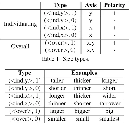
Type Axis Polarity
Individuating
(<ind,y>, 1) y +
(<ind,y>, 0) y
-(<ind,x>, 1) x +
(<ind,x>, 0) x
-Overall (<over>, 1) x,y +
(<over>, 0) x,y
-Table 1: Size types.
Type Examples
(<ind,y>, 1) taller thicker longer
(<ind,y>, 0) shorter thinner short
(<ind,x>, 1) longer thicker wider
(<ind,x>, 0) thinner shorter narrower
(<over>, 1) larger bigger big
(<over>, 0) smaller small smallest
Table 2: Top three surface forms for each size category in the size corpus.
relevant to the scene. For example, with an attribute like SIZE, we know that the dimensional properties of the referent itself must be analyzed in order to de-termine what kind of modifier to produce. Hermann and Deutsch (1976) show that when people are pre-sented with an object with two axes of different sizes than a distractor’s, they are more likely to refer to the axis with the larger difference. Landau and Jackend-off (1993) discuss how a modifier like “big” selects different dimensions depending on the nature of the object, and tends to be used in cases where an object is large in either two or all three of its dimensions, while modifiers like “thick” and “thin” may be ap-plied when an object extends in a single dimension. Brown-Schmidt and Tanenhaus (2006) and Sedivy et al. (1999) document that dimensional modifiers are likely to be used in visual scenes when there is another object of the same type as the target referent.
3 Predicting Size Types
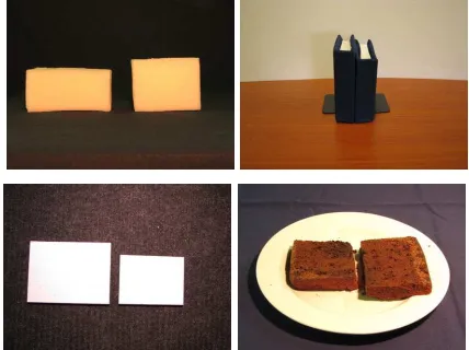
[image:2.612.321.530.58.257.2]Figure 1: Example stimuli in the size corpus (Mitchell et al., 2011a).
examples of corresponding surface forms are listed in Table 2. These types may be used to generate different surface realizations from the same underly-ing semantic form, for example, (<ind,y>, 0) may be used to produce adjectives (“the short box”), rel-ative clauses (“that is shorter”), and prepositional phrases (“with less height”). We refer to these differ-ent kinds of constitudiffer-ents using the broad term modi-fier.
We predict modifiers according to the proposed classes in two domains: A study that specifically elicits size modification (Mitchell et al., 2011b) (the size corpus), and a corpus of instructive reference available from Mitchell et al. (2010) (the craft cor-pus). The size corpus informs the design of the size algorithm and serves as training data for the decision tree models. Example stimuli are given in Figure 1. The algorithm and the decision trees are then tested on a new domain, the craft corpus.
The size algorithm reasons about the difference in the height and width axes between a referent and a distractor to generate a single size modifier type. It is constructed based on the findings listed in Figure 2, and we discuss the algorithm in further detail in the next section. The classifiers use a set of size fea-tures that characterize each image, as well as a set of features reflecting the comparisons made in the hand-coded algorithm. This is discussed in further detail in Section 5.
1. When two dimensions differ in the same direction between a referent object and another object of the same type, an overall size modifier will be produced more often than an individuating size modifier.
2. When two dimensions differ in opposite directions between a referent object and another object of the same type, an individuating size modifier will be produced more often than an overall size modifier.
3. The closer the aspect ratio of an object, the more likely participants are to use an overall size modifier.
Figure 2: Size findings reported in Mitchell et al. (2011b).
4 The Size Algorithm
The size corpus provides information about size when there is a single distractor of the same type, however, in practice, a referent may be competing against several distractors. To address this, the algo-rithm must compare the referent’s height and width against a larger set of heights and widths. A straight-forward way to apply such a comparison is to take the average height and width of the items in the con-trast set. Since size is more common when an item of the same type is in the scene (Brown-Schmidt and Tanenhaus, 2006), it may be suitable for the algo-rithm to compare size using the height and width average of other items of the same type. This also provides a simple way to model the size expecta-tions of the referent relative to similar items. Such an approach is tested in Section 7.
We introduce the size algorithm in Figure 3 below. It is based on the findings listed in Figure 2, and is used when the following preconditions are met:
1. There is a target referent and one or more dis-tractors
2. Each distractor has two dimensions that can be compared with the target referent’s dimensions
As input, the algorithm takes the width and height of the referent (rx, ry) and the width and height of the distractor of the same type or average of the dis-tractors of the same type as the referent (dx, dy). The algorithm outputs one of the size types listed in Table 1.
[image:3.612.321.528.63.182.2]Input: Referent height, width (ry, rx),
Average height, width for distractors of referent’s type (dy, dx).
Output: Size modifier type (See Table 1).
SIZEMOD(rx, ry, dx, dy):
1. axes =<rx, ry, dx, ry>
2. case (mod, pol) of:
3. ry>dy and rx>dx: (<‘over’>, 1)
4. ry>dy and rx<dx: LargestDimDiff(axes)
5. ry>dy and rx == dx: (CalcRatio(axes, ‘y’), 1)
6. ry<dy and rx<dx: (<‘over’>, 0)
7. ry<dy and rx>dx: LargestDimDiff(axes)
8. ry<dy and rx == dx: (CalcRatio(axes, ‘y’), 0)
9. ry == dy and rx>dx: (CalcRatio(axes, ‘x’), 1)
10. ry == dy and rx<dx: (CalcRatio(axes, ‘x’), 0)
11. ry == dy and rx == dx: (None, None)
12. return (mod, pol)
LARGESTDIMDIFF(<rx, ry, dx, dy>):
axis = axis with largest difference between r and d (x or y) pol = direction of difference (0 or 1)
return (<‘ind’, axis>, pol)
CALCRATIO(<rx, ry, dx, dy>, axis): if ry>rx: greater = ry, smaller = rx
else: smaller = ry, greater = rx
p = (greater/smaller) - 1
if p>1: p = 1
v = round(100 * p)
i = random integer between 1 and 100
[image:4.612.315.538.58.313.2]if i>v: mod =<‘over’> else: mod =<‘ind’, axis> return mod
Figure 3: Size algorithm.
Lines 4 and 7 create a structure to generate an indi-viduating size modifier (‘ind’) referring to the axis with the largest difference, with the appropriate po-larity. Here, the modifier type selection reflects the second finding in Figure 2, while the selected axis is chosen based on the conclusions of Hermann and Deutsch (1976).
Lines 5, 8, 9, and 10 are all cases where one axis is different from the distractor and one axis is not. In these cases, following the third finding in Figure 2, we calculate the ratio of difference between the axes (CALCRATIO). This is a stochastic process that models speaker preference for a modifier type as a function of the object’s aspect ratio. The closer the ratio of the x / y axes is to 1, the more likely the algorithm is to generate an overall size modifier.
Line 11 handles the case where both the referent and distractor have the same height and width. In this case, no size modifier is generated.
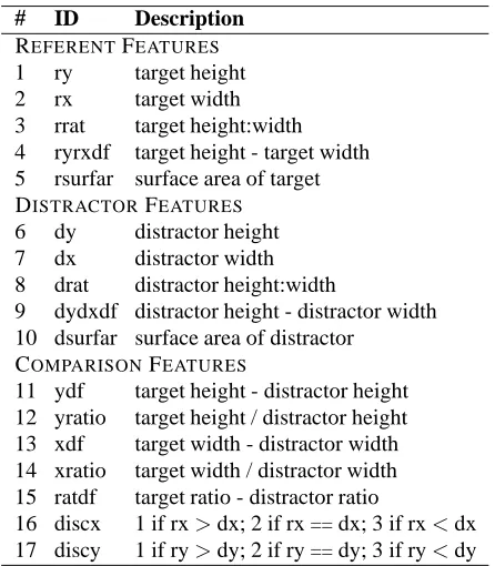
# ID Description
REFERENTFEATURES
1 ry target height
2 rx target width
3 rrat target height:width
4 ryrxdf target height - target width
5 rsurfar surface area of target
DISTRACTORFEATURES
6 dy distractor height
7 dx distractor width
8 drat distractor height:width
9 dydxdf distractor height - distractor width
10 dsurfar surface area of distractor COMPARISONFEATURES
11 ydf target height - distractor height
12 yratio target height / distractor height
13 xdf target width - distractor width
14 xratio target width / distractor width
15 ratdf target ratio - distractor ratio
16 discx 1 if rx>dx; 2 if rx==dx; 3 if rx<dx
17 discy 1 if ry>dy; 2 if ry==dy; 3 if ry<dy
Table 3: Visual features for each expression. Features 16 and 17 mirror the size algorithm’s comparisons.
5 Machine Learning
One of the strengths of applying machine learning to this task is that it may be constructed as a se-ries of binary classification problems, where a model is built for each size type. This allows more than one modifier to be generated for each referent, while avoiding issues of data sparsity inherent in training every combination of size as a separate class. The machine learning approach therefore has functional-ity that the hand-coded size algorithm does not have; it is able to predict sets of modifiers for a referent in-stead of being limited to a single modifier. This flex-ibility is a benefit to the machine learning approach over the hand-coded algorithm, and we return to this issue in Section 8.
To build robust models for this task, we use the data from the experiment in Mitchell et al. (2011a), which includes 414 native or fluent speakers of En-glish. Each expression is annotated to mark the size modifiers and their types (Table 1).
[image:4.612.72.297.92.423.2]im-Type <ind, y> <ind, x> <over>
1 0 1 0 1 0
[image:5.612.319.532.56.267.2]Observed 22 10 3 0 51 43
Table 4: Frequency of observed size modifier types in the craft corpus.
ages are two-dimensional, both annotators reasoned about the three-dimensional shape to resolve refer-ences to all three axes. This is probably especially true for the brownies stimuli due to the angle of the camera, where differences in height may appear to be along the z-axis. In future work, it would be bet-ter to control this aspect, perhaps making only two dimensions visible. For this data, we group those modifiers for z- and y-axes together. Inter-annotator agreement was quite high atκ= 0.94.1
The models are constructed using C4.5 decision tree classifiers as implemented within Weka (Hall et al., 2009), with default parameter settings. We did not find a significant improvement in accuracy on our development set with different pruning meth-ods or normalization. Each feature vector used by the models lists visual size features that characterize each image, such as the size of the referent and dis-tractor’s axes, and differences between the two. We also provide a set of features reflecting the compar-isons made in the hand-coded algorithm. The feature set is listed in Table 3.
6 Testing Corpus
To evaluate how well the models perform in a new domain, we use the craft corpus from the experiment reported in Mitchell et al. (2010). The 2010 exper-iment is a different task, and differs in several criti-cal ways from the 2011 experiment: (1) It was con-ducted in-person, using three-dimensional objects; (2) the referring expressions were produced orally; (3) there were many different objects in the scene, and (4) the objects had a variety of different features: texture, material, color, sheen, etc., as well as size along all three dimensions. A picture of the objects in the experiment is shown in Figure 4. Subjects re-ferred to objects as, for example, “the longer silver ribbon”, and “small green heart”. Table 4 lists the frequency of each observed size type in this corpus.
1729 size modifiers were compared for the agreement score;
[image:5.612.84.289.60.97.2]5 modifiers only labeled by one annotator are excluded.
Figure 4: Object board for craft corpus.
As discussed above, we adapt the size algorithm to the new domain by taking the average height and width of all distractors of the same type, and com-paring the referent against this average. The impli-cations of this are three-fold: (1) Comparisons are limited to those items of the same type; (2) compar-isons are limited to those items in an immediately surrounding group; and (3) comparisons are against a general ‘gist’ of the surrounding scene, instead of individual measurements.
To adapt the classifiers to the new domain, we remove all direct measurement features from train-ing and testtrain-ing; work on our development set sug-gests that including all listed features achieves the best precision and recall when training and testing in the same domain, however, when expanding to a new domain, certain features should be removed for optimal performance. This includes features 1 (ry, target height), 2 (rx, target width), 4 (ryrxdf, target height - width), 6 (dy, distractor height), 7 (dx, dis-tractor width), 9 (dydxdf, disdis-tractor height - width), 11 (ydf, target height - distractor height), 13 (xdf, target width - distractor width). Removing these fea-tures allows the classifiers to build models from rel-ative measurement features alone, and helps mini-mize overfitting to any one domain.
7 Evaluation
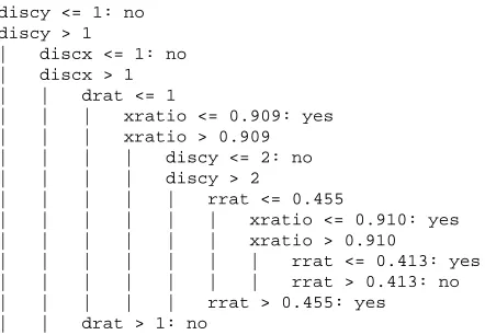
con-discy <= 1: no discy > 1
| discx <= 1: no | discx > 1 | | drat <= 1
| | | xratio <= 0.909: yes | | | xratio > 0.909 | | | | discy <= 2: no | | | | discy > 2
| | | | | rrat <= 0.455
| | | | | | xratio <= 0.910: yes | | | | | | xratio > 0.910
| | | | | | | rrat <= 0.413: yes | | | | | | | rrat > 0.413: no | | | | | rrat > 0.455: yes
[image:6.612.73.294.58.211.2]| | drat > 1: no
Figure 5: Example decision tree: Training on Mechanical Turk data, direct measurement features removed, model
for inclusion of (<over>, 0). Values in cm.
struction of the size algorithm was informed by this corpus, and so this provides a measure of how well the algorithm does in the domain for which it was designed. The decision trees are evaluated in this domain using leave-one-out validation, where the set of expressions for a referent containing at least one size modifier is tested against the models trained on the size expressions for all other referents. An ex-ample tree is shown in Figure 5. Features developed from the hand-coded algorithm (features 16 and 17 in Table 3) appear to have high discriminative utility in the trained models.
Unlike the machine learning approach, the size algorithm generates no more than one size type for each referent, although participants may pro-duce several. To understand the upper bound of both approaches, we therefore implement an oracle method for the size algorithm (ORACLEalg) that al-ways guesses the most common size type for each referent, and an oracle method for the classifiers
(ORACLEtree) that always guesses the most
com-mon set of size types for each referent.
To understand the lower bound, we implement a baseline method that guesses the most common size type and most common set of size types in the train-ing data for each testtrain-ing fold. We find that the most common set of size types across folds contains a single modifier, making the baseline of the two ap-proaches equivalent.
We evaluate the systems using precision and re-call. Since we are comparing the set of predicted modifiers with the set of modifiers that a descrip-tion contains, it would have been possible to use the
Model Mturk Crafts
precision/recall precision/recall
BASELINE 25.7% / 24.5% 16.4% / 16.4%
ORACLEalg 80.5% / 72.7% 89.1% / 89.1%
ORACLEtree 79.5% / 76.0% 89.1% / 89.1%
SIZE
69.7% / 63.4% 81.3% / 81.3%
ALGORITHM
DECISION
65.4% / 65.7% 80.5% / 81.3% TREE
Table 5: Precision and recall for models, testing on ex-pressions that contain size. The size algorithm is aver-aged over 5 iterations.
DICE metric (Dice, 1945), as has often been done in evaluations of REG algorithms (Gatt and Belz, 2008). But DICEdoes not distinguish between re-call (i.e., modifiers that are not predicted but should have been) and precision (i.e., modifiers that are pre-dicted but should not have been), collapsing both of these into one single metric. For our purposes, it will be more informative to separate precision and recall. Given:
Oe= The set of size modifier types observed in an expression e
Pr= The set of size modifier types predicted for a referent r
E= The multiset of expressions in the corpus Er= The multiset of expressions for a referent r
Precision =
X
e∈Er∈E
|Pr∩Oe| |Pr|
|E|
Recall =
X
e∈Er∈E
|Pr∩Oe| |Oe| |E|
Table 5 shows how well the different systems per-form. Testing instances are limited to those that con-tain a size modifier. The second column lists preci-sion and recall on the size corpus. The difference in results between the two systems is not statistically significant.
[image:6.612.316.545.59.188.2]cor-pus contain just one modifier. This also allows a more direct comparison between the two systems, as both the lower bounds (BASELINE) and upper bounds (ORACLE) of the two systems are equal.
As discussed in Section 6, both systems are adapted slightly for the new domain. The size al-gorithm uses the height and width average of items that are the same type as the referent. The decision trees are trained on the full size corpus, and when the models are built from all of the features listed in Table 3, precision / recall on this task is 44.1% / 48.1%. However, once we adapt the classifiers to the subset of relative measurement features, there is a large jump for both measures.
The two systems perform similarly. The size algo-rithm achieves just over 81.3% precision and recall, while the machine learning approach reaches 80.5% precision and 81.3% recall, and the differences be-tween the two methods are not statistically signifi-cant. Oracle accuracy is higher by around 8%, sug-gesting that both systems are reasonable, and further work may want to finesse the kinds of size informa-tion that each uses.
8 Discussion
It is interesting that both systems perform better in the new domain. Both were built based on typed reference to one of two rectilinear solids in a two-dimensional photograph, and still produce reason-able output to spoken reference to one of several three-dimensional objects with different shapes in a much more descriptive task. The two systems likely perform better on the craft corpus than the one they were developed on because in the craft corpus, al-most all expressions contain just one size modifier (only one expression had more).2
The machine learning approach does poorly when it uses the same set of features in both domains, however, by removing those features that may lead to overfitting – the direct measurements of individ-ual objects – it dramatically improves in the new do-main. The difference in precision and recall between the two systems is not statistically significant, with values above 80%.
A notable difference between the two systems is
2This was “the smallest long ribbon”, which both models
fail to predict.
that the machine learning approach can predict any number of size modifiers, while the size algorithm is limited to predicting one modifier (or none). The upper and lower bounds are the same for both in the craft corpus discussed here, however, the classifiers’ ability to predict when several size modifiers will be included may help extend this method in other do-mains.
One immediate question that arises from this work is how to move from abstract size type to sur-face form. For some modifiers, this will be relatively straightforward, but for others, e.g., using (<over>, 1) to generate the phrase “the second largest one”, further functionality must be in place to reason about individual sizes of objects in the contrast set.
Both systems may be developed further by mod-elling speaker variation. Adding speaker label as a feature within the decision tree models guides the construction of distinct speaker clusters (Mitchell et al., 2011b) that generate different kinds of output. Such a technique can be applied here to generate lan-guage for a particular speaker cluster. In this case, the ability of the machine learning approach to gen-erate any number of modifiers may aid in tuning it to specific speaker preferences.
In the size algorithm, speaker variation may be applied several ways. Currently, the algorithm’s CALCRATIO function decides which of the two broad size modifier classes to generate by using a random number generator. This was implemented based on speaker variation in cases where the as-pect ratio of an object approaches 1 (Figure 2). A similar technique may be applied throughout the al-gorithm, where a prior is assigned to various deci-sions based on an analysis of how speakers behave. Another method could apply slightly different ver-sions of the algorithm to different speaker models, where some more detailed aspects of the algorithm are varied for different speaker profiles – for exam-ple, placing a preference on height over width within a threshold of axis size similarity.
9 Conclusions
of size modifier in a realized surface string. Both work relatively well and are extensible to a new do-main.
One of the next clear steps in developing the hand-coded size algorithm is to add functionality for gen-erating sets of modifiers. We would also like to ex-plore different features and the effect they have on the overall accuracy of the different approaches. We hope to address modifiers that pick out specific con-figurations of multiple axes, e.g., “stout” may be re-alized from{(<ind, x>, 1), (<ind, y>, 0)}. Meth-ods for reasoning about the distance and relative ori-entation between the target object and its distractors may guide which axis is referred to, and the systems should be further expanded to real-world objects by adding mechanisms to handle a third z-axis. A bet-ter understanding of when a difference along an axis is small enough not to be salient would help con-nect these approaches more closely to a visual input, placing constraints on when the outlined cases ap-ply.
We hope to address other kinds of properties of real-world referents using a similar methodology, for example, reasoning about the inclusion of spa-tial prepositions between objects. By further defin-ing when different properties are used, how distinct properties interact, and the features affecting their realization, we hope to continue to expand the meth-ods to generate naturalistic reference.
10 Acknowledgments
This research was funded by the Scottish Informat-ics and Computer Science Alliance (SICSA) and the Overseas Research Students Awards Scheme (OR-SAS). Thanks to help from Ellen Bard, Brian Roark, and the anonymous reviewers.
References
Sarah Brown-Schmidt and Michael K. Tanenhaus. 2006. Watching the eyes when talking about size: An investi-gation of message formulation and utterance planning. Journal of Memory and Language, 54:592–609. Robert Dale and Ehud Reiter. 1995. Computational
in-terpretations of the gricean maxims in the generation of referring expressions. Cognitive Science, 19:233– 263.
Lee R. Dice. 1945. Measures of the amount of ecologic
association between species. Ecology, 26(3):297–302, July.
Albert Gatt and Anja Belz. 2008. Attribute selection for referring expression generation: New algorithms and evaluation methods. Proceedings of Fifth Inter-national Natural Language Generation Conference, pages 50–58.
Mark Hall, Eibe Frank, Geoffrey Holmes, Bernhard Pfahringer, Peter Reutemann, and Ian H. Witten. 2009. The weka data mining software: An update. SIGKDD Explorations, 11(1).
Theo Hermann and Werner Deutsch. 1976. Psychologie Der Objektbenennung. Huber Verlag, Bern.
John Kelleher, Fintan Costello, and Josef van Genabith. 2005. Dynamically structuring, updating and interre-lating representations of visual and linguistic discourse context. Artificial Intelligence, 167:62–102.
Ruud Koolen, Martijn Goudbeek, and Emiel Krahmer. 2011. Effects of scene variation on referential over-specification. Proceedings of the 33rd annual meeting of the Cognitive Science Society (CogSci 2011). Emiel Krahmer, Sebastiaan van Erk, and Andr´e Verleg.
2003. Graph-based generation of referring
expres-sions. Computational Linguistics, 29(1):53–72. Barbara Landau and Ray Jackendoff. 1993. “What” and
“where” in spatial language and spatial cognition. Be-havioral and Brain Sciences, 16:217–265.
Margaret Mitchell, Kees van Deemter, and Ehud Reiter. 2010. Natural reference to objects in a visual domain. Proceedings of the Sixth International Natural Lan-guage Generation Conference (INLG-10).
Margaret Mitchell, Kees van Deemter, and Ehud Reiter. 2011a. Applying machine learning to the choice of size modifiers. Proceedings of the 2nd PRE-CogSci Workshop.
Margaret Mitchell, Kees van Deemter, and Ehud Reiter. 2011b. On the use of size modifiers when referring to visible objects. Proceedings of the 33rd Annual Con-ference of the Cognitive Science Society.
Ehud Reiter and Robert Dale. 2000. Building Natural Language Generation Systems. Cambridge University Press.
Julie C. Sedivy, Michael K. Tanenhaus, Craig G. Cham-bers, and Gregory N. Carlson. 1999. Achieving in-cremental semantic interpretation through contextual representation. Cognition, 71:109–147.
Kees van Deemter. 2006. Generating referring expres-sions that involve gradable properties. Computational Linguistics, 32(2):195–222.