Improved Landweber Algorithm Based on Correlation

(1)

ISSN Online: 2153-120X ISSN Print: 2153-1196

DOI: 10.4236/jmp.2017.89093 Aug. 15, 2017 1547 Journal of Modern Physics

Improved Landweber Algorithm Based on

Correlation

Yiqun Kang

*

, Shi Liu

School of Control and Computer Engineering, North China Electric Power University, Beijing, China

Abstract

In order to obtain good effect of image reconstruction of ECT, this paper proposes an ECT image imaging method of improve Landweber algorithm based on data correlation analysis. Using Maxwell simulation software, the method first determines the division of the micro element, then calculates the capacitance of each element as a high dielectric constant, and makes a correla-tion analysis between each capacitance values and the measured capacitance values, a correlation coefficient can be obtained. We can combine the correla-tion coefficient with the sensitive field, and obtain a new sensitive field by us-ing the soft field characteristics of the sensitive field. Combine the new sensi-tive field with the Landweber algorithm to improved image, we can get better imaging of position image.

Keywords

Electrical Capacitance Tomography, Improved Landweber, Correlation Analysis, Reconstruction Sensitive Field

1. Introduction

At present, there are a large number of two-phase flow systems in many fields, such as electricity, petroleum, chemical industry, metallurgy and other national economic production. In these systems, due to the complex flow mechanism of two-phase flow, randomly large, the use of traditional detection technology is difficult to be used for observation or measurement methods. And according to flow pattern change criterion or flow chart to determine the flow mode with the flow parameters is also difficult [1]. So electrical capacitance tomography (ECT) developed gradually since the 1980s.

ECT is an imaging technique, which can measure dielectric constant changes and material distribution in pipes or tubes [2]. It uses differential medium has

How to cite this paper: Kang, Y.Q. and Liu, S. (2017) Improved Landweber Algo-rithm Based on Correlation. Journal of Mo- dern Physics, 8, 1547-1556.

https://doi.org/10.4236/jmp.2017.89093

Received: July 20, 2017 Accepted: August 12, 2017 Published: August 15, 2017

http://creativecommons.org/licenses/by/4.0/

(2)

DOI: 10.4236/jmp.2017.89093 1548 Journal of Modern Physics

different dielectric constant, and by measuring the capacitance values between the electrodes placed on the surface of the tube and the spatial distribution of the dielectric constant in the tube is calculated, combined with the sensitive field, the distribution of the working medium in the pipeline is further deduced. Because ECT can change the position and number of sensor, produce different imaging results, and it does not affect the motion of the fluid, fast, cheap, so it is consi-dered to be the future development prospects of imaging technology [3][4].

In the era of big data, big data can be summarized as four characteristics, data volume, velocity, variety, veracity. Data mining is a technique that looks for re-gularities and rules from a large number of data by analyzing each data, there are three main steps—data preparation, regular search and regular representation. Data preparation is to select the required data from the relevant data source and integrate it into a data set for data mining. The regular search is to find out the rules contained in the data set in some way. The regular representation indicates that the rules are expressed as much as possible in a user-understandable manner (such as visualization). Capacitance data mining process is: first of all data acqui-sition and storage, through the simulation software to get the capacitance value of the filter into a data set when the micro element at high dielectric constant; and then the data set for processing and analysis, such as the use of linear and non-linear statistical analysis of data and according to certain rules of the data set classification, and analyzing the relationships between data and data catego-ries; then the classification of data after data mining, explore and find internal connection between data [5][6]; finally, the results will be imaging, and easy to analyze and use.

Statistics is a comprehensive discipline, which by searching, collating, analyz-ing data and other means to achieve the nature of the measured object, and even predict the future of the object [7]. The regression equation is a mathematical expression that reflects the regression relationship of a variable (dependent vari-able) to another or a set of variables (independent varivari-able) from the sample data by regression analysis. Regression linear equations are used more often, we can use the least squares method to find the regression line equation to get the re-gression linear equation [8].

(3)

data. In this study, it is our intension to investigate the correlation of the permit-tivity distributions with capacitance measurements.

2. The Theoretical Basis

2.1. Principles of Electrical Capacitance Tomography

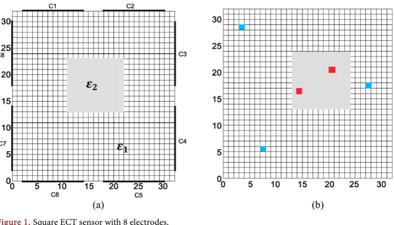
In this paper, a square ECT sensor with 8 electrodes is used [11]. The grid is di-vided into 32 × 32, as shown in Figure 1. Usually, a circle ECT sensor is popular, as a result of this paper uses divided into 32 × 32, and the edge of the circle ECT sensor can not be divided into the same small square, it is not easy to find the correlation. The dielectric constant of the working medium is ε2, and the rest is

1

ε _{. As shown in}_{Figure 1(b)}_{, the blue micro element and the working medium}

do not coincide, we can know that the correlation is small, the red micro element and the working medium coincide, so the correlation is large.

By the definition of the sensitive field:

( )

(

)

(

)

, ,

,

, , 2 1

l i j i j

i j _h _l

i j i j

C e C

S e e

C C

δ

ε ε

− =

− −

(1)

( )

,

( )

,

, ,

l i j i j

h l

i j i j

C e C

C e

C C

− =

− (2)

where Si j,

( )

e is the sensitivity of the e-th test micro element between the i

electrode and the j electrode; Ci j,

( )

e is the capacitance values when the

dielec-tric constant of the e-th element is ε2 and the and the dielectric constant in the

other micro element is ε1, ,

h i j

C and C_{i j}l_, respectively are the capacitance val-ues when the pipeline filled with dielectric constant is ε2 and ε1;

δ

( )

e is a

correction factor related to the area of the e-th unit in the pipeline.

[image:3.595.143.540.493.720.2]

It can be seen from the Equation (1) that there is a certain linear relationship between the Si j,

( )

e and the normalized capacitance value C e

( )

.

(4)

Conventionally, the simulation method is used to obtain the sensitive field. We usually obtain sensitive field by auto Maxwell software. By calculating the internal potential distribution of the pipeline under each excitation voltage, di-rectly using the point multiplication can generally the sensitive field. The specific formula is: ( )

( )

( ) , _, , , d d j i

ij x y _{p x y}

i j

E x y

E x y

S x y

V V

= −

_∫

×

₍₃₎

where E x yi

( )

, is the electric field distribution inside of the pipeline when the

electrode is excited (where the voltage applied to the i electrode is constant Vi),

( )

,

p x y is the area of the pixel in (x, y).

After obtaining the sensitive field by simulation method, by formula (1) we can obtain the capacitance value when the dielectric constant is ε2 in the e-th

element and the dielectric constant in the other micro element are ε1 [12][13].

2.2. Principles of Correlation Coefficient

There are two variables in a linear regression, in which x is an observable and controllable common variable, which is often called an independent variable or controllable variable, and y is a random variable, which is often called a depen-dent variable or a response variable. There is a significant linear correlation be-tween x and y by scattering or calculating the correlation coefficient, that is, the relationship between x and y is as follows [14][15]:

y= +a bx+η (4)

It is usually considered that

(

2

)

~N 0,

η σ _{and suppose}σ2_{has no}

relation-ship with x. Substituting the observed data

(

x yi, i

)

(

i=1,,n

)

into Equation

(4), and note that the sample is a simple random sample, we obtain:

(

)

(

)

1 2

1, ,

, ~ 0,

,

i i i

n

y a bx i n

N

η

η η η σ

= + + =

  



 (5)

Because G=C Sw (G is the pixel gray value), and the Equation (1) can be

written as Equation (6).

( ) (

)

(

)

T

, 2 1

h l l

i j ij ij w k ij

C k = ε −ε ⋅ C −C ⋅C ⋅ ⋅G δ +C (6)

we can simplify Equation (6) as

( )

(

)

T ,

1, , ~ 0, 2

l

i j w ij

n

C k AG C C

N

η

η η η σ

 = ⋅ + +

 

  , (7)

where

(

2 1

)

(

)

h l ij ij k

A= ε −ε ⋅ C −C ⋅δ . The values of a and b (that is l

ij

C and AG) are required to be minimized by:

(

)

2

(

)

2

1 T

1 1

n n

i i i w

i i

Q=

∑

₌ C −C =

∑

₌_C − C +AG C⋅ _ (8)

(5)

(

)

(

) (

)

(

)

( )

(

)

(

)

(

)

(

) (

)(

)

2

T T 1 T

1

2

2 ₂

T T T

1 1 1

2

T T T

1

2

n

i i w w i w

i

n n n

i i w w i i i w

i i i

n

i w i w i w

i

Q C C AG C C C C AGC

C C AG C C AG C C C C

n C a bC C C C C

= = = = =   = _ − − − + − − _   = − + − − − − + − − − −

∑

(9) Let

(

)

(

)

(

)

(

)

(

)

T T T 2 2 T T

, i w w i i

w i

w w i i

i i

C C C C

AG R C C

C C C C

− −

= =

− −

∑

(10)

which reflects the degree of correlation between the two variables. AG is in the range of −1 to 1. Since A is constant, R and G are identically distributed.

( )

1,1 1,28 1 1

2,1 2,28 2 2

1 28

1024,1 1024,28 1024 1024

C e C e R

C w C w

C e C e R

η η η               ₌ __ __₊                               (11)

The new sensitive field matrix constructed by R as weights is:

( )

1 1,1 1 2 1,1 2 1024 1,1 1024

R S e

P e

R S e

P e

R S e

P e  ×        _×    _{ =}         ×         



(12)

( )

1 2

1 1 28

1024

P e P e

G C w C w

P e       =_ __ _       



(13)

2.3. Principles of Improve Landweber Algorithm

The iterative process of the Landweber iteration [16]:

( )k1 ( )k T

(

( )k

)

W

G + =G +αS C −SG (14)

The iterative process of the Landweber iteration based on the correlation ma-trix generated in this study is:

( )1 ( ) T

(

( )

)

1 1 1

k k k

W

G + =G +αP C −PG

(15)

where

α

is iteration step,α =1λmax in simulation, P is the correlation matrix,

and λmax is the maximum eigenvalue of T

P P

.

3. Simulations

3.1. Image Reconstruction by Simulation

(6)

pic-DOI: 10.4236/jmp.2017.89093 1552 Journal of Modern Physics

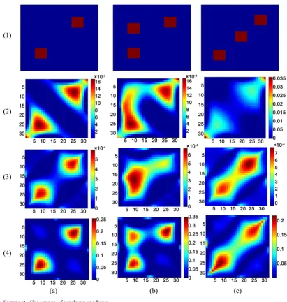
ture, the image map of Landweber algorithm, the image map of correlation algo-rithm, the image map of improved Landweber algorithm based on correlation, the number of iteration is 150.

Various image maps are obtained can be seen from the Figure 2. In Figure 2(a)

Landweber algorithm can separate two square working medium, although the correlation algorithm can not completely separate two square working medium, it can clearly figure out the shape of square. In Figure 2(b) two algorithms can not be imaged correctly, but can only make approximate positions. In Figure 2(c)

[image:6.595.127.539.286.719.2]

the sensitive position of Landweber is not obvious, and the working medium is not imaged at all. In the correlation algorithm, the intensity of the two adjacent working medium is enhanced. The improved Landweber algorithm based on correlation has better imaging effect. In Figure 2(4)-(a), the size of the working medium and the position imaging results are better. In Figure 2(4)-(b) the loca-tion and number of working mediums can be clearly represented.

(7)

3.2. The Sensitivity Analysis by Simulation

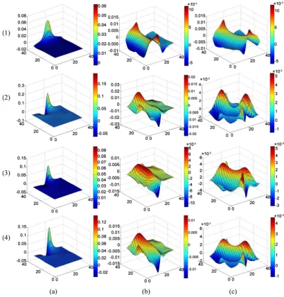
We know that due to the soft field characteristics of the sensitive field, the sensi-tive field will be affected when the working medium is added into the pipeline, which will lead to unsatisfactory imaging results. The results show that the me-thod used in this paper is using the correlation between capacitance and sensitive field, make full use of the soft field characteristic, we can reconstruct the sensi-tive field matrix, and the reconstructed sensisensi-tive field can be regarded as the sen-sitive field after putting into the working medium.

[image:7.595.128.539.279.709.2]

It can be seen from Figure 3, from top to bottom (that is from (1) to (4), of these, (1) is the original sensitive field, (2) to (4) correspond to the case in Figure 2 from (a) to (b)) are the sensitive field between electrodes, from left to right (that is from (a) to (b)) for the sensitive field between the electrodes 1 and 2, electrodes 1 and 6, electrodes 2 and 6. The sensitive field of the working medium

(8)

part is strengthened, so that the imaging effect is better.

3.3. Image Error and Correlation Coefficient

According to the two standards of the image error and image correlation coeffi-cient, a further comparison is made [17]:

ˆ Image error ε ε

ε −

= (13)

(

)

(

)

(

)

1 2

1 1

ˆ Correlation coefficient

ˆ ˆ

n i i

n n

i i

ε ε

ε ε ε ε

=

= =

− =

− −

∑

(14)

where

ε

is the real permittivity distribution,

ε

ˆ is the reconstructed

[image:8.595.207.540.351.729.2]

permit-tivity distribution,

ε

and εˆ are the mean values of

ε

and

ε

ˆ.

Figure 4 is the image error, and Figure 5 is the correlation coefficient. In the

figure, 1 represents Landweber algorithm, 2 represents correlation algorithm, and 3 to 7 represent improved Landweber algorithm based on correlation, the number of iteration is 10, 30, 50, 80, 100. As can be seen from the figure, the im-age error of the correlation algorithm and the improved Landweber significantly

Figure 4. Image error.

(9)

decreased, the correlation coefficient significantly increased. With the increase of the number of iterations, the value of image correlation coefficient tends to be gradual.

4. Conclusion

This paper presents an algorithm based on data analysis and correlation coeffi-cient. The algorithm firstly uses the inverse method to obtain the capacitance value when a certain element is a high dielectric constant working medium, which is simpler and more effective than using the cyclic acquisition method. Comparing with the original sensitive field, it can be found that the recon-structed sensitive field is strengthened in the presence of the working medium, so the imaging effect becomes better. By comparing the image with the Landwe-ber iterative algorithm, it can be seen that the correlation coefficient method has the advantage of reducing the size of the image shape. Improved Landweber al-gorithm based on correlation can improve image quality better, the accuracy of the method of this study is high and the error is small. It is more accurate to de-termine the location of multiple working fluids. It can be seen from the image that the study in the paper is prone to deformation in the diagonal direction, and the future research work should focus on how to modify the image at the di-agonal. And the correlation coefficient method can image the working medium with high dielectric constant, how to make the dielectric constant of the higher working medium imaging better is a key research direction.

References

[1] Yang, W.Q. and Peng, L.H. (2003) Measurement Science and Technology, 14, 1-13. https://doi.org/10.1088/0957-0233/14/1/201

[2] Li, Y. and Holland, D.J. (2013) IEEE Sensors Journal, 13, 446-456. https://doi.org/10.1109/JSEN.2012.2217955

[3] Bai, B.F., Guo, L.J. and Chen, X.J. (2001) Proceedings of the CSEE, 21, 46-50. [4] Lei, J., Liu, S., Li, Z.H. and Sun, M. (2007) Proceedings of the CSEE, 27, 78-83. [5] Han, J., Kamber, M. and Pei, J. (2006) Data Mining: Concepts and Techniques.

Morgan Kaufmann Publishers, San Francisco.

[6] Li, D.R., Wang, S.L. and Li, D.Y. (2013) Spatial Data Mining Theories and Applica-tions. Science Press, Beijing.

[7] Vapnik, V.N. (1995) The Nature of Statistical Learning Theory. Springer-Verlag, New York.

[8] You, J.H., Xu, Q.F. and Zhou, B. (2008) Chinese Annals of Mathematics, 29, 207- 222. https://doi.org/10.1007/s11401-006-0210-8

[9] Li, G.J. and Cheng, X.Q. (2012) Bulletin of Chinese Academy of Sciences, 27, 647- 657.

[10] Liang, J.L., Feng, C.J. and Song, P. (2016) Chinese Journal of Computers, 39, 1-17. [11] Wang, H.X., Tang, L. and Yan, Y. (2007) Chinese Journal of Scientific Instrument,

28, 2014-2018.

(10)

[13] Yang, W.Q., Spink, D.M. and York, T.A. (1999) Measurement Science and Tech-nology, 10, 1065-1069. https://doi.org/10.1088/0957-0233/10/11/315

[14] Guyon, I. and Elisseeff, A. (2003) Journal of Machine Learning Research, 3, 1157- 1182.

[15] Zhang, F., Xie, Z.H. and Cheng, J.T. (2015) Fire Control & Command Control, 40, 83-86.

[16] Landweber, L. (1951) American Journal of Mathematics, 73, 615-624. https://doi.org/10.2307/2372313

[17] Teniou, S. and Meribout, M. (2012) Measurement, 45, 683-690. https://doi.org/10.1016/j.measurement.2011.12.022

Submit or recommend next manuscript to SCIRP and we will provide best service for you:

Accepting pre-submission inquiries through Email, Facebook, LinkedIn, Twitter, etc. A wide selection of journals (inclusive of 9 subjects, more than 200 journals)

Providing 24-hour high-quality service User-friendly online submission system Fair and swift peer-review system

Efficient typesetting and proofreading procedure

Display of the result of downloads and visits, as well as the number of cited articles Maximum dissemination of your research work

Submit your manuscript at: http://papersubmission.scirp.org/