Optimisation in behavioural synthesis using hierarchical expansion: module ripping

Optimisation in behavioural synthesis using hierarchical expansion: module

ripping

A.C. Williams, A.D. Brown and Z. Baidas, Department of Electronics and Computer Science

University of Southampton Hampshire SO17 1BJ

England

Abstract

During behavioural synthesis, an abstract functional description of a system is mapped

automatically onto a physical structure. In a competitive setting, this mapping will be highly

optimised - the dataflow is re-arranged, units and registers are multiplexed and so on - to deliver

a final structure that meets some overall user supplied specification. Ultimately, however, the

physical functional units are drawn from some predefined (human designed) library - these may

be thought of as the leaf-level modules in the design hierarchy.

Design re-use and increasing sophistication of module libraries inevitably leads to leaf

modules becoming larger and more complex. As these modules are, by definition, atomic, a

synthesis system is unable to capitalise on any internal similarities the leaf modules may possess.

This paper describes the design, construction and effects of using a hierarchically defined

module library. The set of leaf-level modules made available to the synthesis environment is

conventional - add, subtract, multiply and so on - but the optimiser is capable of ‘ripping apart’

these modules to manipulate their inner structures.

Two advantages accrue from this technique: (1) it is possible to optimise behavioural

designs far more effectively, with up to a 65% reduction in area, and a 46% reduction in delay

reported, and (2) it is possible to build library modules that have tightly controllable internal

timing relationships. This is essential when designing systems that communicate externally via

low-level protocols, but behavioural synthesis, by its very nature, usually distorts timing

information. Using this technique, it is possible to create ‘islands of fixed timing’ embedded in the

1. Introduction

Behavioural synthesis takes as input a functional description of a design, which specifies the relationship between system input and output in an abstract manner that does not necessarily bear any physical relationship to the final structural physical realisation. The goal of the synthesis system is to translate this behaviour automatically into a structure, optimised such that certain user-specified gross parameters (area, delay, power dissipation) are satisfied.

This paper describes the design and implementation of a hierarchical module expansion capability within the MOODS behavioural synthesis system. Traditionally, each functional (data path) unit in a synthesised design is implemented as a purely combinational logic block taken from a low-level cell/module library. Using ‘expanded modules’ provides a means of

implementing sequential multi-cycle library modules within this model. These modules are defined as technology-independent templates, which are inline expanded into the internal design structure during synthesis. This enables inter-module optimisation to occur at the sub-module level, affording greater opportunities for unit sharing and module binding. The templates also facilitate the development of specialised interface modules - these enable the use of fixed timing I/O protocols for external interfacing, while maintaining maximum scheduling flexibility within the body of the behaviour.

1.1 MOODS (Multiple Objective Optimisation in Data and control path Synthesis)

The MOODS system has been described in detail in [1-5, 16-21]. In summary, MOODS is a system which performs global optimisation of a design dataflow and control graph by the repeated application of small, reversible (behaviour preserving) transforms, controlled by a simulated annealing algorithm. Simulated annealing is used because the problem is a

multivariable optimisation, constrained by a surface (design space) that is discrete, degenerate, discontinuous and contains local minima. Steepest decent type algorithms find this kind of surface notoriously difficult, and taboo search and variations are unsuitable because of the high

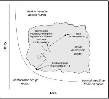
computational cost of back-tracking. The progress of the algorithm may be visualised as a design

space trajectory - the structural design is encapsulated and represented entirely by its coordinates

process is sufficiently fast that the user can sensibly study the various tradeoffs obtainable by exploring the design space.

1.2. Hierarchical module expansion

Early synthesis systems often considered each data path unit to be implemented by a combinational module, executed over a single clock cycle [6]. Later developments utilised more sophisticated characterisation models allowing operations to be either chained together, cascading combinational modules in a single control state, or conversely, multicycling long operations over a number of cycles [7, 8]. In all cases, the modules are treated by synthesis as ‘black boxes’

accompanied simply by area and delay parameters. MOODS handles library modules in a similar manner, treating each as a combinational block with delay, area and power parameters. The transforms applied by the simulated annealing algorithm allow control graph optimisation that results (amongst other things) in operator chaining through the merging of control states, and allows multicycling by means of a user-specified clock period.

Expanded modules are stored as a mixed structural/behavioural description of sub-modules

with their own control and data paths, which are dynamically expanded within the internal design representation at some point during the synthesis process. This enables the use of clocked,

sequential module implementations in-lieu of a single combinational block. The development of a general purpose mechanism for performing hierarchical module expansion also facilitates the implementation of a number of additional features. In particular the ability to pre-define local timing relationships within an expanded module enables the use of macro ports to implement complex interfacing protocols.

1.3 Paper structure

The remainder of the paper is organised as follows: section 2 describes the underlying details of expanded modules and hierarchical expansion, and its effects on the overall optimisation process, while section 3 details the results of an extensive analysis of its operation and

effectiveness on a number of benchmark designs, highlighting the trade-offs and problems encountered. Finally, section 4 identifies key parameters affecting the results of expansion, and describes a semi-automatic algorithm developed to control the process.

2. Expanded modules

descriptions provide performance models, and guide the generation of module structure

independently from the synthesis process. Module expansion, on the other hand, is based on the concept of utilising this hierarchy in the body of the synthesis loop by expanding the sub-structure of a module into its constituent sub-components within the top-level control and data paths. The process involves, by means of a transformation, replacing a given data path unit and its activating control states, by a sub-control and data path that describes the desired module implementation, effectively flattening the module hierarchy. Since expanded modules are described using exactly the same control and data path structures as the rest of the system, there is no restriction on their complexity.

Note that while the majority of transforms employed by MOODS are reversible [1,4], module expansion is only immediately revocable - once any of the substructures have been altered (for example, shared with a unit from another part of the data path either from the top-level

design, or from within another expanded module) the option of ‘unexpanding’ is no longer available (see section 4).

2.1 Sequential module implementation

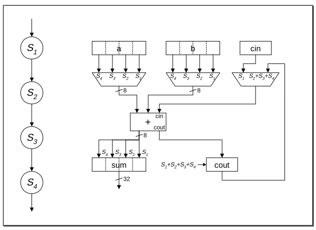
Figure 2 shows a simple example of a single 32-bit combinational adder (executed during a single control state) expanded using a serialised implementation, based around the accumulation of an 8-bit partial sum over four cycles. Three main factors influence the effect a module

expansion such as this has on a synthesised design:

1. The ability to use sequential implementations for a complex operation facilitates an additional level of trade-off between area and delay. This is achieved without any alterations to the low-level module model since the smaller constituent sub-modules are all combinational. The hierarchical nature of the description means that additional trade-offs may be explored by further expanding sub-modules. For example, the 8-bit adder in figure 2 might be further expanded into a serial implementation based around a 2-bit adder, thus increasing the total addition time from 4 to 16 cycles. Clearly, the depth of expansion must be balanced against both the total delay, and the cost of the extra circuitry (multiplexors and intermediate registers) required.

be shorter than the original. This can have a significant impact on the overall speed of the design: by targeting the slowest data path unit for expansion (which dictates the maximum control state delay, and hence the minimum allowed clock period), both the clock period and the amount of unused time in control states can be decreased.

3. Expanded module sub-graphs are merged seamlessly into the top-level design structure, and are treated identically to all other data and control path elements. Further optimisation of the entire design may therefore result in additional improvements through the sharing of sub-modules with other similar data path units. Thus the area cost of a complex operator may in some cases be reduced simply to the overhead incurred by the extra control states, interconnect

(multiplexors) and intermediate registers from the expanded module.

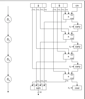
A slightly different approach to the expansion of a 32-bit adder is illustrated in figure 3. Here, the serialised structure is unrolled forming a simple, non-optimal implementation, identical to the initial configuration obtained from a behavioural description of the sequential adder.

At first sight this approach would appear to be more inefficient than before, requiring four separate 8-bit adders and carry registers. However, simply sharing all the adders and all the intermediate carry registers results in a data path structure identical to figure 2. This puts the onus on the synthesis system to draw the maximum benefit from the new configuration through further optimisation, which, while not necessarily the quickest and most computationally efficient

method, possesses a number of advantages over the earlier model:

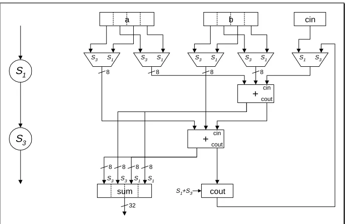
• The expanded modules will be optimised in a manner most suited to the target cost objectives. If this requires maximal unit sharing, the configuration will revert to the original sequential configuration. Alternatively, it may be more appropriate to merge the four control states into two, and similarly share the adders, effectively accumulating a 16-bit partial sum over two cycles, as shown in figure 4. It can therefore be seen that the most important consideration

when designing an expanded module is not its structural efficiency, but the range of

alternative configurations obtainable through further optimisation.

• Feedback loops and unit sharing within the control and data paths makes it much more

difficult for the system to optimise the sub-modules in the context of the whole design, since it would first be necessary to perform data path unit unsharing and control state unrolling

overlapping module execution with other parts of the design is not practical, as the system does not know how many clock cycles it will take for the function to execute - the example in figure 3 makes this parameter explicit by unrolling the calculation loop thus forming a linear control graph whose execution is exactly defined. The system can, however, perform limited functional unit sharing with other parts of the design, thus enabling further area reduction.

• Creation of the expanded module is simply a matter of writing an appropriate behavioural description.

On the negative side, the immediate effect of module expansion on the overall delay and area will almost always be an increase; the expansion process therefore, has to be viewed as a transformation which increases the potential for optimisation at a later date. The problem is complicated by other considerations such as the depth of hierarchy to expand, which units to target, and at what point in the synthesis process the expansion should occur. Section 3 presents experimental data on these issues, and section 4 describes an expansion algorithm developed to tackle them.

2.2 Further uses of expanded modules

As well as the sequential module implementations described above, expansion may be used to provide three additional capabilities: pipelining, macro operators, and macro ports. Traditionally, incorporating these features into a synthesis system would requires specific

modifications to the synthesis algorithms and data structures; using expanded modules, however, enables their inclusion within the structure of the existing system.

2.2.1 Pipelining

Two forms of pipelining applicable to behavioural synthesis are identified in the

literature[8]. Functional pipelining refers to the process of transforming the top-level design into pipelined stages, the execution of which may be overlapped. SEHWA[12], one of the first systems to tackle pipeline synthesis, partitions an acyclic data flow graph into stages separated by stage latches. This increases the rate at which data may be applied to the top-level design, and is best suited to highly repetitive systems such as digital filters. Structural pipelining refers to the use of pipelined modules whose throughput is less than the total module delay. These units require modified scheduling algorithms to overlap pipe stage execution according to the required

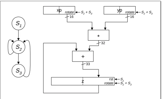
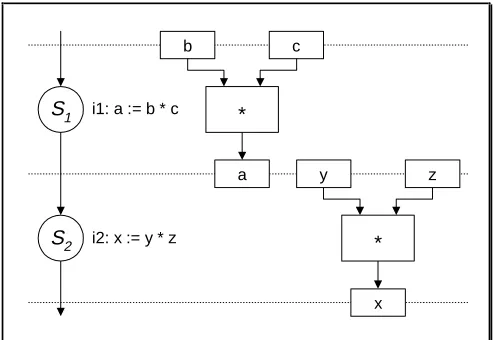
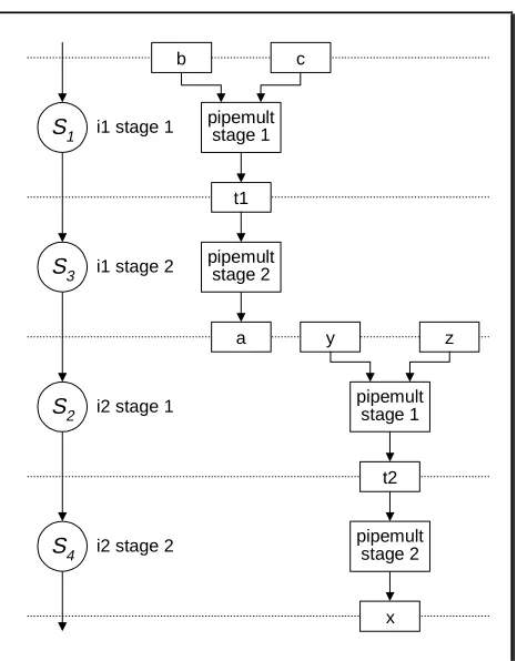
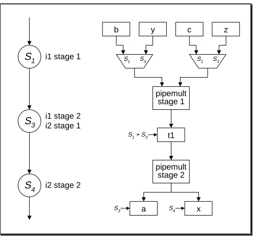
multiply operations (figure 6a) are expanded using a two-stage pipelined multiplier (figure 6b). Given a suitable cost function assigning equal priorities to both area and delay, optimisation results in the configuration of figure 6c, which is the equivalent of performing the two operations on a single pipelined data path unit, overlapping their execution by one cycle.

2.2.2 Macro operators

Expanded modules are also used to implement functions not available in the standard module libraries. These can range from relatively simple individual units, (for example a fixed-point multiplier) to complete complex function libraries, such as to support floating fixed-point arithmetic and transcendental functions. Since the expanded module descriptions are not tied to any specific target library, these macro operators effectively form a high-level function library which seamlessly integrates into the system design flow. This capability is described in detail elsewhere [16-18].

2.2.3 Macro ports

One of the key parameters when controlling module expansion is the point in the

optimisation process at which expansion is performed. This effectively dictates where on the line I-F in figure 1 the expansion is executed (but note that it is not necessary to expand everything at the same time). If this occurs at the end (F in figure 1), just prior to outputting the design as a structural netlist, the expanded control and data path will be directly implemented in the final configuration. This allows the user to exactly specify the local scheduling of operations within the module on a cycle-by-cycle basis (similar to the behavioural templates of [13]).

One of the main drawbacks of behavioural synthesis is the difficulty of interfacing a synthesised design to the outside world, which generally requires the exact specification of operation timing in I/O protocols (for example, memory access control). By encapsulating the required behaviour in an expanded module template with a fixed, pre-defined operation schedule, complex interfaces can be simplified into a single, high-level instruction.

Macro ports also allow a designer to use alternative protocols (for example, faster/slower memory I/O), by simply changing the expanded module used.

This supports a similar interfacing capability to the communication protocol concept found in VHDL+ and SystemC, allowing the body of the design to be optimised without compromising the local timing constraints of the interface.

The operation of an expanded module is coded as a single VHDL process, in an entity whose I/O ports match the pins of the combinational module targeted for expansion. The description should follow standard guidelines for behavioural synthesis, making as little use as possible of signals, except to output the final result at the end of the operation. The use of VHDL enables rapid development in a familiar language, which is easily simulated to ensure correct module operation.

The front end of the synthesis system is, naturally enough, a VHDL parser that translates the input VHDL into an intermediate form, called ICODE: a kind of ‘behavioural assembly language’. Although human readable, in conventional system use this is inspected as frequently as assembly in a high-level software development environment.

The VHDL encoded module is passed through the parser, and translated into ICODE. This may be manually modified to remove unnecessary code or to include additional features with no VHDL parentage, and is then loaded into the synthesis system like any other behavioural design. At this point it can be saved immediately in the expanded module library, or it can be

pre-optimised to obtain any desired structure and schedule. This latter method enables the

development of macro ports with an exactly specified local timing relationship (schedule) that is guaranteed to be maintained in any synthesised design using the module.

Given that the optimisation capabilities of MOODS are underpinned by its ability to manipulate timings, this point is worthy of expansion: In the general course of processing, MOODS modifies the relative timings of operations (without modifying the functionality) within a design unit. In applications, such as those mentioned in section 2.2.3, where fine-grained control over timing is important, MOODS allows the user to 'pin' operations to clock edges by means of special synthesis directives. Syntactically, these look like VHDL procedures, and the library provides simulation models to allow the design to be simulated without modification. (Post optimisation, the procedures have been removed, but the synthesized design is now fully scheduled and obeys the constraints that the pinning procedures imposed at the outset.)

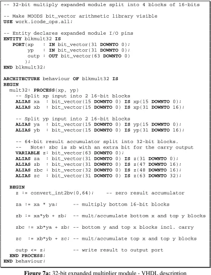
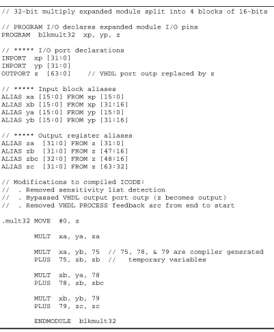
Figure 7 shows an example of this design flow, generating an expanded module for a 32-bit multiplier. Figure 7a shows the generating VHDL, and figure 7b the ICODE equivalent,

modified slightly to remove the sensitivity list detection code, the intermediate output register, and the feedback loop joining the end of the VHDL process to its start. This is then stored as an

unoptimised expanded module with control and data paths as shown in figure 7c.

Using the module structure of figure 7c to expand the multiplier, however, and optimising the entire design for minimum area, the structure of figure 8 is obtained. This has halved the size of the combinational multiplier required, which dominates the size of the implementation. Due to the hierarchical nature of the expansion process, further reduction may be possible by expanding this smaller unit with a similar expanded module, thus decreasing the size of the multiplier to 8 bits. The interaction between this ‘depth of expansion’, and the area and delay figures obtained, is discussed in the next section.

3. Experimental results

The module expansion process must be viewed as a mechanism for enhancing the scope for optimisation, rather than an improvement in its own right. This poses the questions: which modules should be expanded, by how much, and at what stage in the optimisation loop? The results presented here demonstrate the effect various module expansions have on the optimisation of a number of behavioural benchmark designs[14,15]. An analysis of the results shows how the choices made during optimisation affect the final outcome, and examines the interaction with the optimisation algorithm and the effectiveness of the expansion process in general.

From the benchmarks examined, two are analysed in detail here. These designs contain a substantial range of functions of various bit-widths, and are largely data-flow (as opposed to control) oriented. Table 1 describes the two designs in terms of their source code size, and the type and width of operations required. Table 2 lists example area figures for a number of important modules; the size is the number of Cypress FPGA cells (Complex Logic Blocks) required.

Each design is synthesised using a variety of optimisation configurations featuring different expansions of the main arithmetic modules (multiply, add and subtract), and various positions for the expansion operation within the synthesis design flow. These are compared to the non-expanded implementations optimised with respect to area and/or delay. Some multicycled (see section 2.1) optimisations are also included showing the lowest total delay possible through a reduction in the clock period to minimise idle execution time. Tables 3 and 4 summarise selected optimisations for the benchmarks. At various stages in the optimisation, all modules of a particular functional type and bit-width are expanded (or ‘split’). Particular attention is paid to the difference between pre-splitting, that is, expanding modules prior to the first optimisation pass, and

post-splitting, where an initial optimisation is performed before any expansion takes place. For

greater), followed minimal area optimisation; row A3, on the other hand, describes a post-split where first area optimisation is performed, then the multipliers are expanded, all of which is finally followed by a second area optimisation pass.

The execution times are obtained from a P5-100 machine with 32MB memory, running Windows NT 4.0. The total area and delay figures form the performance results, together with the percentage change compared to the non-expanded implementations, i.e. area optimised designs are compared to A1, and delay optimised compared to D1. Breakdowns of these overall figures show the area in terms of the percentage occupied by functional, storage, interconnect and control components, together with the quantity and bit-width of the major arithmetic modules used; and the delay as the critical path length and minimum clock period permitted. The critical path length defines the maximum number of control steps, including loop iterations, in a single execution of the design. In the case of VHDL, this is the time taken by one iteration of the longest process.

The results are summarised in the design spaces of figures 9 and 10. In both designs, the largest functional units are the multiply, add, and subtract modules, are the three types targeted for expansion. The multiplies, in particular, dominate the total area and delay being both the largest and the slowest. Indeed, considering that the largest FPGA used (CY7C387) has only 768 CLBs, it is barely possible to include even a single 16-bit combinational unit (553 CLBs); module expansion is thus essential for any design to fit on a real device of this size.

The design spaces in figures 9 and 10 show the overall effect module expansion can have on the achievable implementations of each design. The non-expanded area and delay points, A1 and D1, delimit the non-expanded optimal design curve. In each case, the expansion process shifts this curve closer to the design space origin, providing a considerably enhanced range of

implementations.

The most obvious characteristic of all the figures is the significant improvement in area of both the area and delay optimised groups, generally, but not always, at the cost of extra delay. The mechanics of this process can be explained by looking at the area distribution between the

functional, storage, interconnect and control components. All the non-expanded implementations (A1, AM, D1, DM) exhibit a substantial functional unit bias comprising between 65% and 95% of the total area. This is primarily due to the large combinational multipliers and the inherent data-centric nature of the designs. Module expansion reduces the size of the functional component due to the reduced complexity of the constituent sub-units, in return for an increase in storage,

cancels out any functional block decreases, rendering the expansion ineffective. A3 and A4 in figure 10 clearly illustrate this point: the first configuration (A3) shows post-split expansion of all 16-bit multipliers achieving a 26% decrease in total area, from a 71% decrease in functional area, and a 28%, 100% and 118% increase in storage, interconnect and control area respectively, compared to the non-expanded A1. Expanding a further level of hierarchy with post-split optimisation of all 16 and 8-bit multipliers (A4), results in a less significant 12% total decrease, this time comprising an 88% drop in functional area, but a 36%, 213% and 596% increase in the other three.

Another, less obvious, effect of expansion is an improvement in the overall clock

utilisation. The longest functional unit propagation delay determines the minimum clock period, leading to the waste of a considerable amount of excess time inside many control states.

Multicycling attacks this inefficiency by allowing combinational modules to evaluate over several cycles, thereby reducing the clock period and improving the overall delay figure. Comparing the original implementations (A1 and D1) with their multicycled equivalents (AM and DM), it can be seen that the decrease in clock period is accompanied by an increase in the critical path length; multicycling serves to balance out these two components, achieving a more even distribution of functional unit execution time across the available control states. The greater number of control states also affects the area, but this is not accompanied by any change in the other area

components as multicycling simply modifies the control graph. Examination of the delay breakdown for the expanded configurations exhibits a similar pattern.

Finally, figure 11 shows the clock utilisation distribution for the system of figure 10. For optimum clock utilisation, the majority of states should occupy the top 95-100% range, but the original non-expanded configuration (A1) falls far short of this target, with over 65% of states having a utilisation of around 60%. The best multicycled implementation (AM) is a far more efficient scenario with 90% of states almost 100% utilised. In between these two extremes appear the expanded implementations demonstrating a varying degree of improvement. Note that figure 11 only shows the utilisation efficiency; better utilisation does not necessarily mean a lower total delay as both the clock period and critical path length may vary, but it does indicate how much time is wasted in a given schedule. It is interesting to note that in every configuration there exists at least one state with a very low utilisation - these represent VHDL wait statements forming points at which a process is idle: no substantial operations will be scheduled here resulting in a low utilisation figure. The subject of clock and module utilisation is discussed further in [2, 21].

In its entirety, MOODS is a highly complex software suite, providing numerous synthesis capabilities not described here [1-5,16-21]. Presenting a unified, comprehensible and useful interface to the user is becoming more and more difficult with each added enhancement. At the outset, the decision was taken to use simulated annealing as the overarching control algorithm, as it is ideally suited to balancing nonlinear, nonmonotonic and occasionally discontinuous tradeoffs between disparate penalty functions. While this has proved to be a wise decision, controlling the system is not simple. Ideally, the control of any complex system is implemented with the

minimum number of independent parameters, each affecting a well defined (and preferably

independent) set of aspects of the output.

In the case of module expansion, there are a number of parameters affecting the process that must be controlled by the optimisation algorithm. Specifically, it must:

• determine which data path units in the design should be expanded

• determine which expanded module implementations should be used

• determine when, during optimisation, expansion should occur (pre/post splitting)

In making these decisions, there are two key problems which must be overcome: first, the initial effect of expanding a module is often an increase in both area and delay, and it is only after

further optimisation that the true effects of the expansion can be ascertained; second, once

expansion has occurred, and the module’s sub-structure has been further optimised and integrated into the top-level control and data-paths, it is unfeasible to undo (ie. backtrack and replace the expanded implementation by the original single functional unit) as this would require the

automatic reconstruction of the module’s control and data-path substructure - a process that would be both difficult to perform, and extremely time consuming, for the following reasons:

A key feature of the system is that a complete (i.e. fully scheduled, bound and allocated) design exists after every transform. The repercussions of each transform, although localised in the control/datapath graph sense, touch large parts of the software data structure, which is extremely complex. For this reason, it is infeasible to maintain a strict backtrace of the system progress, even over short distances. Transforms are reversed by applying the corresponding 'anti-transform', that has the opposite effect on the design (but does not necessarily restore the data structure to its exact original state). The anti-transform corresponding to module expansion would be a subgraph isomorphism problem. Whilst the addition to the transform lexicon of such a process is possible, it would have a completely unacceptable impact on the performance of the synthesis system.

returning the system to the original point in the design space, rather than a new point outside the local minimum.

The expansion process must therefore be viewed as an irreversible transform that increases the potential for further optimisation at a later time.

Despite close scrutiny of the results both in tables 3-5 and elsewhere[3], it has not been possible to derive a sensible detailed heuristic to encapsulate and fully control the expansion process. However, a number of experimental observations can be made:

• There is little to be gained (even using a priori knowledge) from treating the functional units separately.

• Intuitively, it would seem that splitting as early as possible (ie. at the outset) would move the design space closer to the origin, and produce better designs. This means, however, that the initial post-expansion design can be very large and complex, particularly when using large macro operators (such as floating-point units) which can considerably slow down the optimisation process. Results show that multi-stage splitting (ie. performing several expansions at various stages throughout synthesis) can produce comparable results with a much reduced runtime.

• All this notwithstanding, the designs produced using module splitting are demonstrably superior to those produced without (figures 9 and 10).

The approach taken in MOODS is to provide a degree of automatic expansion, but require the user to take ultimate control of the process. This method enables the effects of expansion to be investigated at various stages of the optimisation process. The automatic hierarchical expansion algorithm enables the user to expand all functional units of a particular operation type for a specific bit-width range, and provides the facility to override the expansion for individual units where necessary. The user can also specify how many levels of hierarchy are expanded, thus it is possible to perform a first pass expansion, where only the required top-level functional units are expanded, then perform some optimisation, and then perform more expansion - ie. trade off pre-/post-splitting.

Although it has not been possible to fully automate the optimisation and expansion process in a single algorithm, a general approach to design optimisation, using a mixture of automatic optimisation and manual intervention, can be developed thus:

1. Perform standard non-expanded optimisation to investigate the design space and determine minimum feasible area and delay figures.

3. Perform one-level pre- and post-split optimisations to gauge the possible effects of expansion. If a functional path unit is shared among operations of varying bit-width, it may be necessary to unshare some of these prior to post-splitting.

4. Repeat the expansion process based on the new dominant functional unit, or with more levels of expansion, until the desired area is obtained, the area starts to increase, or the delay exceeds some maximum allowed limit.

These steps should form the basis upon which a more detailed optimisation configuration can be developed, possibly involving the consideration of some individual units, and the

manipulation of cost function target values.

In addition to automatic hierarchical expansion, the system provides the ability to manually expand individual functional units, and also to force the expansion of all macro operators. This is necessary since macro operators generally have no simple functional unit equivalent (ie. combinational implementation), and thus must be expanded before synthesis is complete. Providing the user with the ability to perform this operation means that a multi-pass approach can be taken where early optimisation treats the complex operators as ‘black boxes’, enabling higher-level optimisation, while later, post-expansion stages perform the detailed intra- and inter-module optimisation.

5. Summary

The development of a module expansion capability within the architecture of the existing synthesis system enables further optimisation of a behavioural design, primarily as a mechanism for decreasing the area occupied by the final implementation. It enables the system to utilise sequential clocked modules in place of the original purely combinational units, allowing much more substantial designs to be developed within the constraints imposed by the resources of FPGA devices. Expanding the hierarchical structure of a module within the top-level control and data paths allows the system to perform inter-module optimisations further reducing the area requirements. The expansion process also tends to reduce the complexity (and hence delay) of the slowest functional modules, thus improving the clock utilisation through a lower minimum clock period.

References

1. Baker K.R., Currie A.J. and Nichols K.G., “Multiple Objective Optimisation in a

Behavioural Synthesis System”, IEE Proceedings - Circuits Devices & Systems, Vol. 140, August 1993, pp. 253-260.

2. Brown A.D., Baker K. R. and Williams A.C., “Online Testing of Statically and Dynamically Scheduled Synthesized Systems”, IEEE Transactions on Computer-Aided Design, Vol. 16, No. 1, January 1997, pp. 47-57.

3. Williams A.C., “A Behavioural VHDL Synthesis System using Data Path Optimisation”,

PhD thesis, University of Southampton, UK, October 1997.

4. Baker K.R., Brown A.D. and Currie A.J., “Optimisation Efficiency in Behavioural

Synthesis”, IEE Proceedings - Circuits Devices & Systems, Vol. 141, No. 5, October 1994, pp. 399-406.

5. Baker K.R., “Multiple Objective Optimisation of Data and Control Paths in a Behavioural Silicon Compiler”, PhD thesis, University of Southampton, UK, September 1992.

6. Parker A.C., Mlinar M., Pizarro J., “MAHA: A Program for Datapath Synthesis”,

Proceedings of the 23rd ACM/IEEE Design Automation Conference, July 1986, pp. 461-466.

7. Peng Zebo, “Synthesis of VLSI Systems with the CAMAD Design Aid”, Proceedings of the

23rd ACM/IEEE Design Automation Conference, 1986, pp. 278-284.

8. Paulin P.G., Knight J.P., “Force-Directed Scheduling for the Behavioral Synthesis of ASIC’s”, IEEE Transactions on Computer-Aided Design, Vol. 8, No. 6, June 1989, pp. 661-679.

9. Wolf W., “An Object-Oriented, Procedural Database for VLSI Chip Planning”, Proceedings

of the 23rd ACM/IEEE Design Automation Conference, 1986, pp. 744-751.

10. Müzner A., “Building block Generation Considering the Inherent Hierarchy of Arithmetic Operations”, Proceedings IFIP Working Conference on Logic and Architecture Synthesis, May 1990, pp. 297-306.

11. Müzner A., “BADGE - A Synthesis Tool for Customized Arithmetic Building Blocks”, IFIP

Transactions A - Computer Science and Technology, Vol. A-22, 1993, pp. 359-371.

12. Park N., Parker A.C., “SEHWA: A Software Package for Synthesis of Pipelines from Behavioral Specifications”, IEEE Transactions on Computer-Aided Design, Vol. 7, No. 3, March 1988, pp. 356-370.

13. Ly T., Knapp D., Miller R., MacMillen D., “Scheduling using Behavioral Templates”,

Proceedings of the 32nd ACM/IEEE Design Automation Conference, Session 7, 1995.

15. Vemuri R., Roy J., Mamtora P., Kumar N., “Benchmarks for High Level Synthesis”, Laboratory for Digital Design Environments, University of Cincinnati, 1991.

16. Brown, A.D. and Baidas, Z., EPSRC grant reference GR/L28494 final report, “High level Floating Point Synthesis Library”.

17. Williams, A.C., Brown, A.D., Zwolinski, M., “Simultaneous Optimisation of Dynamic Power, Area and Delay in Behavioural Synthesis”, IEE proceedings on Computers and

Digital Techniques, Vol. 147, No. 6, November 2000.

18. Baidas, Z., Brown A.D. and Williams, A.C., “A VHDL Behavioural Synthesis System with Floating Point Support”, Forum on Design Languages 2000 (FDL 2000)7 ELQJHQ

Germany.

19. Nijhar, T.P.K., and Brown, A.D., “Source Level Optimisation of VHDL for Behavioural Synthesis”, IEE proceedings on Computers and Digital Techniques, Vol. 144, No. 1, January 1997, pp. 1-6.

20. Nijhar, T.P.K., and Brown, A.D., “HDL-Specific Source Level Behavioural Optimisation”,

IEE proceedings on Computers and Digital Techniques, Vol. 144, No. 2, March 1997, pp.

138-144.

Figure and table captions

Figure 1: A two-dimensional projection (area/delay) of behavioural design space Figure 2: Expanded 32-bit serial adder

Figure 3: Expanded 32-bit split adder

Figure 4: Example optimisation of 32-bit split adder Figure 5: 32-bit block multiplier expanded module Figure 6: Pipelined multiply operations

Figure 6a: Two sequentially scheduled multiply operations

Figure 6b: Multipliers expanded using 2-stage pipelined expanded modules Figure 6c: Optimum schedule/sharing forming a single pipelined multiplier Figure 7: Development of a 32-bit multiplier expanded module

Figure 7a: 32-bit expanded multiplier module - VHDL description

Figure 7b: 32-bit expanded multiplier module - modified ICODE description Figure 7c: Initial post-expansion control and data paths for 32-bit multiplier Figure 8: The single multiplier process optimised for area

Figure 9: DIFFEQ expanded design space Figure 10: ELLIP expanded design space

Figure 11: Various ELLIP clock utilisation distributions Table 1: Benchmark design size and operator usage figures Table 2: Sample module sizes for various bit-widths

optimal area/time trade-off curve unachievable design

region

ideal achievable design region

actual achievable

region

Area

De

la

y

initial implementation (I)

final optimised implementation (F) optimisation

trajectory: each point represents a different

structural implementation

b cin

cout S₂

S₁

S₁+S₂+S₃+S₄

+ cin

cout S₃

S₄ S₁

sum S

4 S3 S2 S1

S₂ S₁ a

S₃

S₄ S₂ S₁ S₂+S₃+S₄

S₄ S₃

8 8

8

32

sum

carry

carry

carry b

a

+_coutcin

cin

+ cin

cout

+ cin

cout

+_coutcin

cout S₂

S₃ S₁

S₄

S4 S3 S2 S1

S4

S3

S2

S₁ 8

8 8

8 8 8 8 8

8 8

8 8

32

b

a cin

cout

S₃ S₁

S1+S3

+_coutcin

+ cin cout

S3 S1 S3 S1

S3 S1 S3 S1 S1 S3

sum S3 S3 S1 S1

32 8 8 8 8

8 8 8 8

yp xp

+ *

z rst S1

S₂ S₁

S₃

32

33

16 16

rotate S₂ + S₃ rotate

rotate S₂ + S₃ S₂ + S₃

a

b c

* i1: a := b * c

i2: x := y * z S₁

S₂

x

y z

*

i1 stage 1

i1 stage 2 S₁

S₃

i2 stage 1

i2 stage 2 S₂

S₄

a

b c

pipemult stage 1

pipemult stage 2

x

y z

pipemult stage 1

pipemult stage 2 t1

t2

i1 stage 1

i1 stage 2 i2 stage 1 S₁

S₃

i2 stage 2 S₄

a

pipemult stage 1

pipemult stage 2

t1

x

b y c z

S1 S3 S1 S3

S1 + S3

S3 S4

Figure 7a: 32-bit expanded multiplier module - VHDL description

-- 32-bit multiply expanded module split into 4 blocks of 16-bits

-- Make MOODS bit_vector arithmetic library visible

USE work.icode_ops.all;

-- Entity declares expanded module I/O pins

ENTITY blkmult32 IS

PORT(xp : IN bit_vector(31 DOWNTO 0); yp : IN bit_vector(31 DOWNTO 0); outp : OUT bit_vector(63 DOWNTO 0) );

END blkmult32;

ARCHITECTURE behaviour OF blkmult32 IS BEGIN

mult32: PROCESS(xp, yp)

-- Split xp input into 2 16-bit blocks

ALIAS xa : bit_vector(15 DOWNTO 0) IS xp(15 DOWNTO 0); ALIAS xb : bit_vector(15 DOWNTO 0) IS xp(31 DOWNTO 16);

-- Split yp input into 2 16-bit blocks

ALIAS ya : bit_vector(15 DOWNTO 0) IS yp(15 DOWNTO 0); ALIAS yb : bit_vector(15 DOWNTO 0) IS yp(31 DOWNTO 16);

-- 64-bit result accumulator split into 32-bit blocks. -- Note: zbc is zb with an extra bit for the carry output VARIABLE z: bit_vector(63 DOWNTO 0);

ALIAS za : bit_vector(31 DOWNTO 0) IS z(31 DOWNTO 0); ALIAS zb : bit_vector(31 DOWNTO 0) IS z(47 DOWNTO 16); ALIAS zbc : bit_vector(32 DOWNTO 0) IS z(48 DOWNTO 16); ALIAS zc : bit_vector(31 DOWNTO 0) IS z(63 DOWNTO 32);

BEGIN

z := convert_int2bv(0,64); -- zero result accumulator

za := xa * ya; -- multiply bottom 16-bit blocks

zb := xa*yb + zb; -- mult/accumulate bottom x and top y blocks

zbc := xb*ya + zb; -- bottom y and top x blocks incl. carry

zc := xb*yb + zc; -- mult/accumulate top x and top y blocks

outp <= z; -- write result to output port END PROCESS;

Figure 7b: 32-bit expanded multiplier module - modified ICODE description

// 32-bit multiply expanded module split into 4 blocks of 16-bits

// PROGRAM I/O declares expanded module I/O pins PROGRAM blkmult32 xp, yp, z

// ***** I/O port declarations INPORT xp [31:0]

INPORT yp [31:0]

OUTPORT z [63:0] // VHDL port outp replaced by z

// ***** Input block aliases ALIAS xa [15:0] FROM xp [15:0] ALIAS xb [15:0] FROM xp [31:16] ALIAS ya [15:0] FROM yp [15:0] ALIAS yb [15:0] FROM yp [31:16]

// ***** Output register aliases ALIAS za [31:0] FROM z [31:0] ALIAS zb [31:0] FROM z [47:16] ALIAS zbc [32:0] FROM z [48:16] ALIAS zc [31:0] FROM z [63:32]

// Modifications to compiled ICODE: // . Removed sensitivity list detection

// . Bypassed VHDL output port outp (z becomes output) // . Removed VHDL PROCESS feedback arc from end to start

.mult32 MOVE #0, z

MULT xa, ya, za

MULT xa, yb, 75 // 75, 78, & 79 are compiler generated PLUS 75, zb, zb // temporary variables

MULT xb, ya, 78 PLUS 78, zb, zbc

MULT xb, yb, 79 PLUS 79, zc, zc

S₂ S₁ S₄ S₃ S₆ S₅ S₈ S₇ i1 i2 i3 i4 i5 i6 i7 i8 32 yp xp + * 75 * + * 78 + * 79 z S₅ S₃ S₇ S 2 S

4+S6

S 8 S₆ S₁ cout rst 16 16 16 16 32 32 32 32 16 16 16 16 32 32 32 32 32

16

yp xp

+ * S₂+S₃

S₅+S₇ S₃+S₇ S₂+S₅

z S2

S3+S5

S7

S₅

S1

rst S₃+S₅

S₇ S₂

S₁

S₅ S₃

S₇ i1

i2

cout i3

i4

i5

i6

i7

i8

16

32 32

32

16 16 16 16

16 16 16

16

DIFFEQ - optimised design space

0 5 10 15 20 25

0 1000 2000 3000 4000 5000 6000 7000 8000 9000 10000

Area (CLBs)

Delay (

µ

s)

Original Area optimised Delay optimised Multicycled

A4 A5

A6

A7

A3 A2

A8

A1 D1

DM D9

D10 D2

D8

D3 D6 D4

D7 D5

A9 A11

A10

N(14105,5.7)

ELLIP - optimised design space

0 2 4 6 8 10 12 14 16

0 200 400 600 800 1000 1200 1400 1600

Area (CLBs)

Delay (

µ

s)

Original Area optimised Delay optimised Multicycled

D4

A6 A5

D2

D3 D1

DM D5

D6

A3 A2

A4 A8

A7

A1

D7

AM

N(5712,6.6)

ELLIP - clock utilisation distribution 0 10 20 30 40 50 60 70 80 90 100

0-5 _5-10

10-15 15-20 20-25 25-30 30-35 35-40 40-45 45-50 50-55 55-60 60-65 65-70 70-75 75-80 80-85 85-90 90-95 95-100

Clock utilisation (%)

Number

of contr

o

l states (%)

A1 A6 A7 AM

Design Lines of Operators (quantity x bit-width)

name VHDL Operations plus Minus mult ls le ne

DIFFEQ 108 36 2 × 32 2 × 32 6 × 32 2 × 1 1 × 32

ELLIP 100 50 26 × 16 8 × 16 1 × 16

Bit-width (n) Register 2 input multiplexor Ripple-carry adder Multiplier

8-bit 8 CLBs 2.4 CLBs 12 CLBs 138 CLBs 16-bit 16 CLBs 4.8 CLBs 24 CLBs 553 CLBs 32-bit 32 CLBs 9.6 CLBs 48 CLBs 2212 CLBs 64-bit 64 CLBs 19.2 CLBs 96 CLBs 8847 CLBs

Func Store Inter Cont

unoptimised N - 14105 - 95.7 3.9 0.2 0.2 2x(+,32) 2x(-,32)

6x(*,32) 5.7 - 22 257.3

area optimised A1 1 2856 0.0 81.5 14.6 3.5 0.4 1x(+/-,32) 1x(*,32) 3.1 0.0 9 342.9

pre-split (*,32), area optimised A2 13 1680 -41.2 39.8 36.3 22.0 1.9 1x(+/-,32) 1x(*,16) 7.1 128.7 31 227.7

post-split (*,32), area optimised A3 11 1543 -46.0 43.3 33.4 21.2 2.1 1x(+/-,32) 1x(*,16) 7.3 136.0 32 227.7

pre-split (*,16), area optimised A4 440 1730 -39.4 14.6 37.2 40.7 7.4 1x(+/-,32) 1x(*,8) 20.8 574.0 127 163.8

post-split (*,16), area optimised A5 898 1502 -47.4 16.8 36.5 37.8 8.9 1x(+/-,32) 1x(*,8) 21.6 600.6 132 163.8

post-split (*,32), area optimised, split (*,16), area optimised

A6 416 1607 -43.7 15.8 34.3 41.9 8.0 1x(+/-,32) 1x(*,8) 21.0 579.4 128 163.8

post-split (*,32), (+,32) & (-,32),

area optimised A7 28 1824 -36.1 34.4 32.5 30.0 3.1 1x(+/-,16) 1x(*,16) 11.0 257.8 55 200.7

post-split (+,32) & (-,32), area

optimised A8 1 2881 0.9 79.4 14.7 5.4 0.5 1x(+/-,16) 1x(*,32) 3.8 22.8 12 315.8

pre-split (+,32) & (-,32), area

optimised A9 2 2888 1.1 79.2 14.7 5.6 0.5 1x(+/-,16) 1x(*,32) 4.3 37.7 14 303.6

post-split (*,32_32), area

optimised A10 5 1260 -55.9 53.0 30.7 14.1 2.1 1x(+/-,32) 1x(*,16) 5.9 91.6 26 227.4

post-split (*,16_16), area

optimised A11 117 1023 -64.2 24.7 39.5 26.9 8.9 1x(+/-,32) 1x(*,8) 14.6 374.0 90 162.5

delay optimised D1 1 9630 0.0 94.2 4.7 1.1 0.1 1x(-,32) 1x(+/-,32)

4x(*,32) 1.5 0.0 5 303.6

pre-split (*,32), delay optimised D2 1 2560 -73.4 54.4 24.0 20.4 1.2 3x(+,32) 1x(-,32)

2x(*,16) 4.1 170.6 29 141.7

post-split (*,32), delay

optimised D3 5 2534 -73.7 51.3 26.8 20.7 1.2 2x(+/-,32) 2x(*,16) 4.3 180.0 30 141.7

pre-split (*,16), delay optimised D4 675 2117 -78.0 21.5 29.8 42.8 5.9 2x(+,32) 1x(-,32)

2x(*,8) 9.5 523.7 124 76.4

post-split (*,16), delay

optimised D5 370 2326 -75.9 24.4 28.6 41.6 5.5 2x(+/-,32) 2x(*,8) 11.1 633.6 127 87.7

post-split (*,16), delay

optimised, delay optimised D6 582 2420 -74.9 27.4 27.4 39.9 5.2 2x(+/-,32) 2x(*,8) 9.7 535.8 126 76.6

post-split (*,32), delay optimised, split (*,16), delay optimised, delay optimised

D7 175 2437 -74.7 28.2 28.6 38.8 4.5 1x(+,16) 2x(+/-,32)

2x(*,8) 8.2 442.9 108 76.3

post-split (*,32), (+,32) & (-,32), delay optimised, split (*,16), delay optimised

D8 171 2249 -76.6 17.4 32.8 43.9 5.8 2x(+/-,16) 2x(*,8) 9.9 553.6 130 76.3

post-split (+,32) & (-,32), delay

optimised D9 12 7407 -23.1 92.2 5.8 1.8 0.2

2x(+,16) 3x(-,16)

1x(+/-,16) 3x(*,32) 2.8 86.4 11 257.3

' delay cf. A1,D1 (%) CPU (secs) CPL (states) Clock (ns) Area Breakdown (%)

Module Usage Delay (µs) Optimisation

configuration Ref

Area (CLBs)

' area cf. A1,D1 (%)

Func Store Inter Cont

unoptimised N - 5712 - 88.5 10.7 0.0 0.8 26x(+,16) 8x(*,16) 6.6 - 47 141.4

area optimised A1 9 918 0.0 63.9 24.5 8.6 2.9 1x(+,16) 1x(*,16) 8.6 0.0 27 319.0

pre-split (*,16), area optimised A2 68 826 -10.0 20.8 42.7 29.3 7.1 1x(+,16) 1x(*,8) 6.7 -21.7 59 114.3

post-split (*,16), area optimised A3 69 681 -25.8 25.2 42.5 23.6 8.7 1x(+,16) 1x(*,8) 6.8 -21.6 59 114.4

post-split (*,8), area optimised A4 1868 810 -11.8 8.4 37.7 30.7 23.2 1x(+,16) 1x(*,4) 14.3 66.2 188 76.1

post-split (*,16), target area

optimised (90000) A5 30 726 -20.8 30.6 42.0 18.8 8.5 1x(+,16) 1x(*,8) 4.7 -45.4 62 75.8

post-split (*,16), delay

optimised A6 18 927 1.1 38.3 34.6 22.1 5.0 2x(+,16) 2x(*,8) 4.7 -45.9 46 101.2

post-split (*,16), area optimised, split (*,8), area optimised

A7 1992 1025 11.7 6.6 36.0 39.7 17.7 1x(+,16) 1x(*,4) 13.8 60.1 181 76.2

pre-split (*,8), area optimised A8 3850 925 0.7 7.4 36.5 36.0 20.2 1x(+,16) 1x(*,4) 14.2 65.0 187 76.0

area optimised, multicycled (20

ns) AM 9 1157 26.0 50.7 19.5 6.8 23.0 1x(+,16) 1x(*,16) 5.3 -38.2 266 20.0

delay optimised D1 3 1556 0.0 76.3 14.5 8.2 1.1 3x(+,16) 2x(*,16) 2.4 0.0 17 141.5

pre-split (*,16), delay optimised D2 16 1101 -29.3 34.7 32.1 29.3 3.9 4x(+,16) 2x(*,8) 3.2 35.0 43 75.5

post-split (*,16), delay

optimised D3 12 1080 -30.6 35.4 34.2 26.6 3.9 4x(+,16) 2x(*,8) 3.2 31.8 42 75.5

post-split (*,8), delay optimised D4 527 1101 -29.2 15.8 32.8 36.0 15.4 4x(+,16) 2x(*,8) 7.1 193.6 170 41.6

post-split (*,16), area optimised D5 57 886 -43.1 24.8 39.8 30.1 5.3 3x(+,16) 1x(*,8) 5.4 123.1 47 114.2

post-split (*,16), delay optimised, split (*,8), delay optimised

D6 266 1170 -24.8 15.9 32.2 39.4 12.5 1x(+,8) 4x(+,16)

2x(*,4) 6.0 148.6 146 41.0

pre-split (*,8), delay optimised D7 909 1283 -17.5 15.3 29.4 41.9 13.5 4x(+,16) 2x(*,4) 7.0 189.0 173 40.2

delay optimised, multicycled

(70 ns) DM 4 1577 1.3 75.3 14.3 8.1 2.4 3x(+,16) 2x(*,16) 1.5 -36.8 38 40.0

Area Breakdown (%) Optimisation

configuration Ref

Area (CLBs)

' area cf. A1,D1 (%) CPU (secs) CPL (states) Clock (ns) Delay (µs)

Module Usage ' delay cf. A1,D1 (%)