Proceedings of the NAACL HLT Workshop on Unsupervised and Minimally Supervised Learning of Lexical Semantics, pages 54–62,
Using DEDICOM for
Completely Unsupervised Part-of-Speech Tagging
Peter A. Chew, Brett W. Bader
Sandia National Laboratories
P. O. Box 5800, MS 1012
Albuquerque, NM 87185-1012, USA
{pchew,bwbader}@sandia.gov
Alla Rozovskaya
Department of Computer Science
University of Illinois
Urbana, IL 61801, USA
[email protected]
Abstract
A standard and widespread approach to part-of-speech tagging is based on Hidden Markov Models (HMMs). An alternative approach, pioneered by Schütze (1993), induces parts of speech from scratch using singular value decomposition (SVD). We introduce DEDICOM as an alternative to SVD for part-of-speech induction. DEDICOM retains the advantages of SVD in that it is completely unsupervised: no prior knowledge is required to induce either the tagset or the associations of types with tags. However, unlike SVD, it is also fully compatible with the HMM framework, in that it can be used to esti-mate emission- and transition-probability matrices which can then be used as the input for an HMM. We apply the DEDICOM method to the CONLL corpus (CONLL 2000) and compare the output of DEDICOM to the part-of-speech tags given in the corpus, and find that the cor-relation (almost 0.5) is quite high. Using DEDICOM, we also estimate part-of-speech ambiguity for each type, and find that these estimates correlate highly with part-of-speech ambiguity as measured in the original corpus (around 0.88). Finally, we show how the output of DEDICOM can be evaluated and compared against the more familiar output of supervised HMM-based tagging.
1
Introduction
Traditionally, part-of-speech tagging has been ap-proached either in a rule-based fashion, or stochas-tically. Harris (1962) was among the first to develop algorithms of the former type. The rule-based approach relies on two elements: a dictio-nary to assign possible parts of speech to each word, and a list of hand-written rules – which must be painstakingly developed for each new language or domain – to disambiguate tokens in context. Stochastic taggers, on the other hand, avoid the need for hand-written rules by tabulating probabili-ties of types and part-of-speech tags (which must be gathered from a tagged training corpus), and applying a special case of Bayesian inference (usually, Hidden Markov Models [HMMs]) to dis-ambiguate tokens in context. The latter approach was pioneered by Stolz et al. (1965) and Bahl and Mercer (1976), and became widely known through the work of e.g. Church (1988) and DeRose (1988).
A third and more recent approach, known as ‘distributional tagging’ and exemplified by Schütze (1993, 1995) and Biemann (2006), aims to eliminate the need for both hand-written rules and a tagged training corpus, since the latter may not be available for every language or domain. Distri-butional tagging is fully-unsupervised, unlike the two traditional approaches described above. Schütze suggests analyzing the distributional pat-terns of words by forming a term adjacency matrix, then subjecting that matrix to Singular Value De-composition (SVD) to reveal latent dimensions. He shows that in the reduced-dimensional space im-plied by SVD, tokens do indeed cluster intuitively by part-of-speech; and that if context is taken into account, something akin to part-of-speech tagging
can be achieved. Whereas the performance of sto-chastic taggers is generally sub-optimal when the domain of the training data differs from that of the test data, distributional tagging sidesteps this prob-lem, since each corpus can be considered in its own right. Schütze (1995) notes two general draw-backs of distributional tagging methods: the per-formance is relatively modest compared to that of supervised methods; and languages with rich mor-phology may pose a challenge.1
In this paper, we present an alternative unsuper-vised approach to distributional tagging. Instead of SVD, we use a dimensionality reduction technique known as DEDICOM, which has various advan-tages over the SVD-based approach. Principal among these is that, even though no pre-tagged corpus is required, DEDICOM can easily be used as input to a HMM-based approach (and the two share linear-algebraic similarities, as we will make clear in section 4). Although our empirical results, like those of Schütze (1995), are perhaps still rela-tively modest, the fact that a clearer connection exists between DEDICOM and HMMs than be-tween SVD and HMMs gives us good reason to believe that with further refinements, DEDICOM may be able to give us ‘the best of both worlds’ in many respects: the benefits of avoiding the need for a pre-tagged corpus, with empirical results ap-proaching those of HMM-based tagging.
In the following sections, we introduce DEDICOM, describe its applicability to the part-of-speech tagging problem, and outline its connec-tions to the standard HMM-based approach to tag-ging. We evaluate the use of DEDICOM on the CONLL 2000 shared task data, discuss the results and suggest avenues for improvement.
2
DEDICOM
DEDICOM, which stands for ‘DEcomposition into DIrectional COMponents’, is a linear-algebraic decomposition method attributable to Harshman (1978) which has been used to analyze matrices of
1
We note the latter is also true for languages in which word order is relatively free – usually the same languages as those with rich morphology. While English word order is signifi-cantly constrained by part-of-speech categorizations, this is not as true of, say, Russian. Thus, an adjacency matrix formed from a Russian corpus is likely to be less informative about part-of-speech classifications as one formed from an English corpus. Quite possibly, this is as much of a limitation for DEDICOM as it is for SVD.
asymmetrical directional relationships between objects or persons. Early on, the technique was applied by Harshman et al. (1982) to the analysis of two types of marketing data: ‘free associations’ – how often one phrase (describing hair shampoo) evokes another in the minds of survey respondents, and ‘car switching data’ – how often people switch from one to another of 16 car types. Both datasets are asymmetric and directional: in the first dataset, for example, the phrase ‘body’ (referring to sham-poo) evoked the phrase ‘fullness’ twice as often in the minds of respondents as ‘fullness’ evoked ‘body’. Likewise, the data from Harshman et al. (1982) show that in the given period, 3,820 people switched from ‘midsize import’ cars to ‘midsize domestic’ cars, but only 2,140 switches were made in the reverse direction. Another characteristic of these ‘asymmetric directional’ datasets is that they can be represented in square matrices. For exam-ple, the raw car switching data can be represented in a 16 ×16 matrix, since there are 16 car types.
The objective of DEDICOM, which can be compared to that of SVD, is to factorize the raw data matrices into a lower-dimensional space iden-tifying underlying, idealized directional patterns in the data. For example, while there are 16 car types in the raw car switching data, Harshman shows that under a 4-dimensional DEDICOM analysis, these can be ‘boiled down’ to the basic types ‘plain large-midsize’, ‘specialty’, ‘fancy large’, and ‘small’ – and that patterns of switching among these more basic types can then be identified.
If X represents the original n × n matrix of asymmetric relationships, and a general entry xij in
X represents the strength of the directed relation-ship of object ito object j, then the single-domain DEDICOM model2can be written as follows:
X = ARAT+ E (1)
where A denotes an n×qmatrix of weights of the nobserved objects in q dimensions (where q< n), and R is a dense q×qasymmetric matrix express-ing the directional relationships between the q di-mensions or basic types. ATis simply the transpose
2
of A, and E is a matrix of error terms. Our objec-tive is to minimize E, so we can also write:
X ARAT (2)
As noted by Harshman (1978: 209), the fact that A appears on both the left and right of R means that the data is described ‘in terms of asymmetric relations among a single set of things’ – in other words, when objects are on the receiving end of the directional relationships, they are still of the same type as those on the initiating end.
One difference between DEDICOM and SVD is that there is no unique solution: either A or R can be scaled or rotated without changing the goodness of fit, so long as the inverse operation is applied to the other. For example, if we let  = AD, where D is any diagonal scaling matrix (or, more generally, any nonsingular matrix), then we can write
X ARAT= ÂD-1RD-1ÂT (3) since ÂT= (AD) T = DAT
(In our application, we constrain A and R to be nonnegative as noted below.)
To our knowledge, there have been no applica-tions of DEDICOM to date in computational lin-guistics. This is in contrast to SVD, which has been extensively used for text analysis (for appli-cations other than unsupervised part-of-speech tagging, see Baeza-Yates and Ribeiro-Neto 1999).
3
Applicability of DEDICOM to
part-of-speech tagging
Schütze’s (1993) key insight is that – at least in English – adjacencies between types are a good guide to their grammatical functions. That insight can be leveraged by applying either SVD or DEDICOM to a type-by-type adjacency matrix. With DEDICOM, however, we add the constraint (already stated) that the types are a ‘single set of things’: whether a type ‘precedes’ or ‘follows’ – i.e., whether it is in a row or a column of the ma-trix – does not affect its grammatical function. This constraint is as it should be, and, to our knowledge, sets DEDICOM apart from all previous unsuper-vised approaches including those of Schütze (1993, 1995) and Biemann (2006).
Given any corpus containing n types and k to-kens, we can let X be an n × n token-adjacency
matrix. Let each entry xij in X denote the number
of times in the corpus that type iimmediately pre-cedes type j. X is thus a matrix of bigram frequen-cies. It follows that the sum of the elements of X equals k– 1 (because the first token in the corpus is preceded by nothing, and the last token is fol-lowed by nothing). Any given row sum of X (the type frequency corresponding to the particular row) will equal the corresponding column sum, except if the type happens to occur in the first or last position in the corpus. X will be asymmetric, since the frequency of bigram ij is clearly not the same as that of bigram ji for all iand j.
It can be seen, therefore, that our X represents asymmetric directional data, very similar to the data analyzed in Harshman (1978) and Harshman et al. (1982). If we fit the DEDICOM model to our X matrix, then we obtain an A matrix which represents types by latent classes, and an R matrix which represents directional relationships between latent classes. We can think of the latent classes as induced parts of speech.
With SVD, we believe that the orthogonality of the reduced-dimensional features militates against any attempt to correlate these features with parts of speech. From a linguistic point of view, there is no reason to believe that parts of speech are orthogon-al to one another in any sense. For example, nouns and adjectives (traditionally classified together as ‘nominals’) seem to share more in common with one another than nouns and verbs. With DEDICOM, this is not an issue, because the col-umns of A are not required to be mutually ortho-gonal to one another, unlike the left and right singular vectors from SVD.
Thus, the A matrix from DEDICOM shows how strongly associated each type is with the different induced parts of speech; we would expect types which are ambiguous (such as ‘claims’, which can be either a noun or a verb) to have high loadings on more than one column in A. Again, if the classes correlate with parts of speech, the R matrix will show the latent patterns of adjacency between different parts of speech.
4
Connections between DEDICOM and
HMM-based tagging
part-of-speech tagging, the tags are conceived of as the hidden layer of the HMM and the tokens (each of which is associated with a type) as the visible layer. The emission probabilities are then the prob-abilities of types given the tags, and the transition probabilities are the probabilities of the tags given the preceding tags. If these probabilities are known, then there are algorithms (such as the Vi-terbi algorithm) to determine the most likely se-quence of tags given the visible sese-quence of types. In the case of supervised learning, we obtain the emission and transition probabilities by observing actual frequencies in a tagged corpus. Suppose our corpus, as previously discussed, consists of ntypes and ktokens. Since we are dealing with supervised learning, the number of the tags in the tagset is also known: we denote this number q. Now, the ob-served frequencies can be represented, respective-ly, as n×qand q×qmatrices: we denote these A* and R*. Each entry aij in A* denotes the number of
times type iis associated with tag j, and each entry rij in R* denotes the number of times tag j
imme-diately follows tag i. Moreover, we know some other properties of A* and R*:
• the respective sums of the elements of A* and R* are equal to k– 1;
• each row sum of A* (
=
q
x ix
a
1) corresponds to
the frequency in the corpus of type i;
• each column sum of A*, as well as the corres-ponding row and column sums of R*, are the frequencies of the given tags in the corpus (for
all j,
= =
=
=
= q
x jx q
x xj q
x
xj r r
a
1 1
1
).
If A* and R* contain frequencies, however, we must perform a matrix operation to obtain transi-tion and emission probabilities for use in an HMM-based tagger. In effect, A* must be made column-stochastic, and R* must be made row-stochastic. Since the column sums of A* equal the respective row sums of R*, this can be achieved by post-multiplying both A* and R* by DA, where DA
is a diagonal scaling matrix containing the inverses of the column sums of A (or equivalently, the row sums of R). Then the matrix of emission probabili-ties is given by A*DA, and the matrix of transition
probabilities by R*DA.
We can now make the connection to DEDICOM explicit. Let A = A*DAand R = R*, then we can
rewrite (2) as follows:
X ARAT= (A*DA) R* (A*DA) T
(4) X A*DAR*DAA*
T
(5)
In other words, for any corpus we may compute a probabilistic representation of the type adjacency matrix X (which will contain expected frequencies comparable to the actual frequencies) by multiply-ing the emission probability matrix A*DA, the
transition probability matrix R*DA, and the
type-by-tag frequency matrix A*. (Presumably, the closer the approximation, the better the tagging in the training set actually factorizes the true direc-tional relationships.)
Conversely, for fully unsupervised tagging, we can fit the DEDICOM model to the type adjacency matrix X. The resulting A matrix contains esti-mates of what the tags should be (if a tagged train-ing corpus is unavailable), as well as the emission probability of each type given each tag, and the resulting R matrix is the corresponding transition probability matrix given those tags. In this case, a column-stochastic A can be used directly as the emission probability matrix, and we simply make R* row-stochastic to obtain the matrix of transition probabilities. The only difference then between the output of the fully-unsupervised DEDICOM/HMM tagger and that of a supervised HMM tagger is that in the first case, the ‘tags’ are numeric indices representing the corresponding column of A, and in the second case, they are the members of the tagset used in the training data.
The fact that emission and transition probabili-ties (or at least something very like them) are a natural by-product of DEDICOM sets DEDICOM apart from Schütze’s SVD-based approach, and is for us a significant reason which recommends the use of DEDICOM.
5
Evaluation
in the work described here. The tags are from a 44-item tagset. The CONLL 2000 tags against which we measure our own results are in fact assigned by the Brill tagger (Brill 1992), and while these may not correlate perfectly with those that would have been assigned by a human linguist, we believe that the correlation is likely to be good enough to allow for an informative evaluation of our method.
Before discussing the evaluation of unsuper-vised DEDICOM, let us briefly reconsider the si-milarities of DEDICOM to the supervised HMM model in the light of actual data in the CONLL corpus. We stated in (5) that X A*DAR*DAA*
T
. For the CONLL 2000 tagged data, A* is a 19,440
× 44 matrix and R* is a 44 × 44 matrix. Using A*DA and R*DA as emission- and
transition-probability matrices within a standard HMM (where the entire CONLL 2000 corpus is treated as both training and test data), we obtained a tagging accuracy of 95.6%. By multiplying A*DAR*DAA*
T
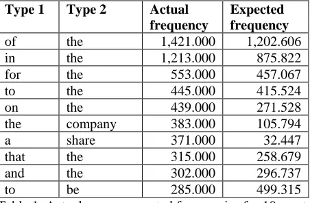
, we expect to obtain a matrix ap-proximating X, the table of bigram frequencies. This is indeed what we found: it will be apparent from Table 1 that the top 10 expected bigram fre-quencies based on this matrix multiplication are generally quite close to actual frequencies. Moreo-ver, the sum of the elements in A*DAR*DAA*
T
is equal to the sum of the elements in X, and if we let
E be the matrix of error terms (X -
A*DAR*DAA* T
), then we find that ||E|| (the Frobe-nius norm of E) is 38.764% of ||X|| - in other words, A*DAR*DAA*Taccounts for just over 60%
of the data in X.
Type 1 Type 2 Actual frequency
Expected frequency
of the 1,421.000 1,202.606 in the 1,213.000 875.822 for the 553.000 457.067 to the 445.000 415.524 on the 439.000 271.528 the company 383.000 105.794
a share 371.000 32.447
[image:5.612.74.300.502.650.2]that the 315.000 258.679 and the 302.000 296.737 to be 285.000 499.315 Table 1. Actual versus expected frequencies for 10 most common bigrams in CONLL 2000 corpus
Having confirmed that there exists an A (=A*DA) and R (=R*) which both satisfies the
DEDICOM model and can be used directly within
a HMM-based tagger to achieve satisfactory re-sults, we now consider whether A and R can be estimated if no tagged training set is available.
We start, therefore, from X, the square 19,440 × 19,440 (sparse) matrix of raw bigram frequencies from the CONLL 2000 data. Using Matlab and the Tensor Toolbox (Bader and Kolda 2006, 2007), we computed the best rank-44 non-negative DEDICOM3 decomposition of this matrix using the 2-way version of the ASALSAN algorithm presented in Bader et al. (2007), which is based on iteratively improving random initial guesses for A and R. As with SVD, the rank of the decomposi-tion can be selected by the user; we chose 44 since that was known to be the number of items in the CONLL 2000 tagset, but a lower number could be selected for a coarser-grained part-of-speech anal-ysis. Ultimately, perhaps the best way to determine the optimal rank would be to evaluate different options within a larger end-to-end system, for ex-ample an information retrieval system; this, how-ever, was beyond our scope in this study.
As already mentioned, there are indeterminacies of rotation and scale in DEDICOM. As Harshman et al. (1982: 211) point out, ‘when the columns of A are standardized… the R matrix can then be in-terpreted as expressing relationships among the dimensions in the same units as the original data.
That is, the R matrix can be interpreted as a ma-trix of the same kind as the original data mama-trix X, but describing the relations among the latent as-pects of the phrases, rather than the phrases them-selves’. Thus, if DEDICOM is constrained so that A is column-stochastic (which is required in any case of the matrix of emission probabilities), then the sum of the elements in R should approximate the sum of the elements in X. R is therefore com-parable to R* (with some provisos which shall be enumerated below), and to obtain the row-stochastic transition-probability matrix, we simply multiply R by a diagonal matrix DR whose
ele-ments are the inverses of R’s row sums.
3
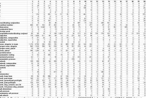
Table 2. Partial confusion matrix of gold-standard tags against DEDICOM-induced tags for CONLL 2000 dataset
With A as an emission-probability matrix and RDR as a transition-probability matrix, we now
have all that is needed for an HMM-based tagger to estimate the most likely sequence of ‘tags’ given the corpus. However, since the ‘tags’ here are nu-merical indices, as mentioned, to evaluate the out-put we must look at the correlation between these ‘tags’ and the gold-standard tags given in the CONLL 2000 data. One way this can be done is by presenting a 44 × 44 confusion matrix (of gold-standard tags against induced tags), and then mea-suring the correlation coefficient (Pearson’s R) between that matrix and the ‘idealized’ confusion matrix in which each induced tag corresponds to one and only one ‘gold standard’ tag. Using A and RDR as the input to a HMM-based tagger, we
tagged the CONLL 2000 dataset with induced tags and obtained the confusion matrix shown in Table 2 (owing to space constraints, only the first 20 col-umns are shown). The correlation between this matrix and the equivalent diagonalized ‘ideal’ ma-trix is in fact 0.4942, which is significantly higher than could have occurred by chance.
It should be noted that a lack of correlation be-tween the induced tags and the gold standard tags can be attributed to at least two independent fac-tors. The first, of course, is any inability of the DEDICOM model to fit the particular problem and data. Clearly, this is undesirable. The other factor to be borne in mind, which works to DEDICOM’s favor, is that the DEDICOM model could yield an A and R which factorize the data more optimally than the A*D and R* implied by the gold-standard tags. There are three methods we can use to try and tease apart these competing explanations of the results, two quantitative and the other subjective. Quantitatively, we can compare the respective er-ror matrices E. We have already mentioned that
38764 . 0 ||
X ||
|| A D R D A X
|| * A * A *T
(6)
Similarly, using the A and R from DEDICOM we can compute
24078 . 0 ||
X ||
|| ARA X
|| T
The fact that the error is lower in the second case implies that DEDICOM allows us to find a part-of-speech ‘factorization’ of the data which fits better even than the gold standard, although again there are some caveats to this; we will return to these in the discussion.
Another way to evaluate the output of DEDICOM is by comparing the number of part-of-speech tags for a type in the gold standard to the number of classes in the A matrix with which the type is strongly associated. We test this by measur-ing the Pearson correlation between the two va-riables. First, we compute the average number of part-of-speech tags per type using the gold stan-dard. We refer to this value as ambiguity coeffi-cient; for the CONLL dataset, this is 1.05. Because A is dense, if we count all non-zero columns for a type in the A matrix as possible classes, we obtain a much higher ambiguity coefficient. We therefore set a threshold and consider only those columns whose values exceed a certain threshold. The thre-shold is selected so that the ambiguity coefficient of the A matrix is the same as that of the gold stan-dard. For a given type, every column with a value exceeding the threshold is counted as a possible class for that type. We then compute the Pearson correlation coefficient between the number of classes for a type in the A matrix and the number of part-of speech tags for that type in the CONLL dataset as provided by the Brill tagger. We ob-tained a correlation coefficient of 0.88, which shows that there is indeed a high correlation be-tween the induced tags and the gold standard tags obtained with DEDICOM.
Finally, we can evaluate the output subjectively by looking at the content of the A matrix. For each ‘tag’ (column) in A, the ‘types’ (rows) can be listed in decreasing order of their weighting in A. This gives us an idea of which types are most
cha-racteristic of which tags, and whether the grouping into tags makes any intuitive sense. These results (for selected tags only, owing to limitations of space) are given in Table 3.
Many groupings in Table 3 do make sense: for example, the fourth tag is clearly associated with verbs, while the two types with significant weight-ings for tag 2 are both determiners. By referring back to Table 2, we can see that many tokens in the CONLL 2000 dataset tagged as verbs are indeed tagged by the DEDICOM tagger as ‘tag 4’, while many determiners are tagged as ‘tag 3’. To under-stand where a lack of correlation may arise, how-ever, it is informative to look at apparent anomalies in the A matrix. For example, it can be seen from Table 3 that ‘new’, an adjective, is grouped in the third tag with ‘a’ and ‘the’ (and ranking above ‘an’). Although not in agreement with the CONLL 2000 ‘gold standard’ tagging, the idea that determiners are a type of adjective is in fact in accordance with traditional English gram-mar. Here, the grouping of ‘new’, ‘a’ and ‘the’ can be explained by the distributional similarities (all precede nouns). It should also be emphasized that the A matrix is essentially a ‘soft clustering’ of types (meaning that types can belong to more than one cluster). Thus, for example, ‘u.s.’ (the abbrevi-ation for United States) appears under both tag 2 (which appears to have high loadings for nouns) and tag 8 (with high loadings for adjectives).
We have alluded above in passing to possible methods for improving the results of the DEDICOM analysis. One would be to pre-process the data differently. Here, a variety of options are available which maintain a generally unsupervised approach (one example is to avoid treating punctu-ation as tokens). However, varipunctu-ations in pre-processing are beyond the scope of this paper.
Tag Top 10 types (by weight) with weightings
1 million share said . year billion inc. corp. years quarter 0.0246 0.0146 0.0129 0.0098 0.0088 0.0069 0.0064 0.0061 0.0058 0.0054 2 company u.s. new first market share year stock . government
0.0264 0.0136 0.0113 0.0095 0.0086 0.0086 0.0079 0.0077 0.0065 0.006 3 the a new an other its any addition their 1988
0.2889 0.1194 0.0121 0.0094 0.0092 0.0085 0.0067 0.0062 0.0062 0.0057 …
[image:7.612.72.559.567.693.2]8 the its his about those their all u.s. . this 0.0935 0.0462 0.0208 0.0160 0.0096 0.0095 0.0088 0.0077 0.0074 0.0071 …
Another method would be to constrain DEDICOM so that the output more closely models the characteristics of A* and R*, the emission- and transition-probability matrices obtained from a tagged training set. In particular, there is one im-portant constraint on R* which is not replicated in R: the constraint mentioned above that for all j,
= =
=
q xjx q
x
xj
r
r
1 1. We note that this constraint can be
satisfied by Sinkhorn balancing (Sinkhorn 1964)4, although it remains to be seen how the constraint on R can best be incorporated into the DEDICOM architecture. Assuming that A is column-stochastic, another desirable constraint is that the rows of A(DR)
-1
should sum to the same as the rows of X (the respective type frequencies). With the implementation of these (and any other) con-straints, one would expect the fit of DEDICOM to the data to worsen (cf. (6) and (7) above), but in-curring this cost could be worthwhile if the payoff were somehow linguistically interesting (for ex-ample, if it turned out we could achieve a much higher correlation to gold-standard tagging).
6
Conclusion
In this paper, we have introduced DEDICOM, an analytical technique which to our knowledge has not previously been used in computational linguis-tics, and applied it to the problem of completely unsupervised part-of-speech tagging. Theoretical-ly, the model has features which recommend it over other previous approaches to unsupervised tagging, specifically SVD. Principal among the advantages is the compatibility of DEDICOM with the standard HMM-based approach to part-of-speech tagging, but another significant advantage is the fact that types are treated as ‘a single set of objects’ regardless of whether they occupy the first or second position in a bigram.
By applying DEDICOM to a tagged dataset, we have shown that there is a significant correlation between the tags induced by unsupervised, DEDICOM-based tagging, and the pre-existing gold-standard tags. This points both to an inherent validity in the gold-standard tags (as a reasonable
4It is also worth noting that Sinkhorn was motivated by the same problem which concerns us, that of estimating a transi-tion-probability matrix for a Markov model.
factorization of the data) and to the fact that DEDICOM appears promising as a method of in-ducing tags in cases where no gold standard is available.
We have also shown that the factors of DEDICOM are interesting in their own right: our tests show that the A matrix (similar to an emis-sion-probability matrix) models type part-of-speech ambiguity well. Using insights from DEDICOM, we have also shown how linear alge-braic techniques may be used to estimate the fit of a given part-of-speech factorization (whether in-duced or manually created) to a given dataset, by comparing actual versus expected bigram frequen-cies.
In summary, it appears that DEDICOM is a promising way forward for bridging the gap be-tween unsupervised and supervised approaches to part-of-speech tagging, and we are optimistic that with further refinements to DEDICOM (such as the addition of appropriate constraints), more in-sight will be gained on how DEDICOM may most profitably be used to improve part-of-speech tag-ging when few pre-existing resources (such as tagged corpora) are available.
Acknowledgements
We are grateful to Danny Dunlavy for contributing his thoughts to this work.
References
Brett W. Bader, Richard A. Harshman, and Tamara G. Kolda. 2007. Temporal analysis of semantic graphs using ASALSAN. In Proceedings of the 7th IEEE In-ternational Conference on Data Mining, 33-42. Brett W. Bader and Tamara G. Kolda. 2006. Efficient
MATLAB Computations with Sparse and Factored Tensors. Technical Report SAND2006-7592, Sandia National Laboratories, Albuquerque, NM and Liver-more, CA.
Brett W. Bader and Tamara G. Kolda. 2007. The MATLAB Tensor Toolbox, version 2.2. http://csmr.ca.sandia.gov/~tgkolda/TensorToolbox/. Ricardo Baeza-Yates and Berthier Ribeiro-Neto. 1999.
Modern Information Retrieval. New York: ACM Press.
L. R. Bahl and R. L. Mercer. 1976. Part of speech as-signment by a statistical decision algorithm. In Pro-ceedings of the IEEE International Symposium on Information Theory, 88-89.
C. Biemann. 2006. Unsupervised part-of-speech tagging employing efficient graph clustering. In Proceedings of the COLING/ACL 2006 Student Research Work-shop, 7-12.
E. Brill. 1992. A simple rule-based part of speech tag-ger. In Proceedings of the Third Conference on Ap-plied Natural Language Processing, 152-155. K. W. Church. 1988. A stochastic parts program and
noun phrase parser for unrestricted text. In ANLP 1988, 136-143.
CONLL 2000. Shared task data. Retrieved Dec. 1, 2008 from http://www.cnts.ua.ac.be/conll2000/chunking/. S. J. DeRose. 1988. Grammatical category
disambigua-tion by statistical optimizadisambigua-tion. Computational Lin-guistics 14, 31-39.
Harris, Z. S. 1962. String Analysis of Sentence Struc-ture. Mouton: The Hague.
Richard Harshman. 1978. Models for Analysis of Asymmetrical Relationships Among N Objects or Stimuli. Paper presented at the First Joint Meeting of the Psychometric Society and The Society for Ma-thematical Psychology. Hamilton, Canada.
Richard Harshman, Paul Green, Yoram Wind, and Mar-garet Lundy. 1982. A Model for the Analysis of Asymmetric Data in Marketing Research. Marketing Science 1(2), 205-242.
Hinrich Schütze. 1993. Part-of-Speech Induction from Scratch. In Proceedings of the 31stAnnual Meeting of the Association for Computational Linguistics, 251-258.
Hinrich Schütze. 1995. Distributional Part-of-Speech Tagging. In Proceedings of the 7th Conference of the European Chapter of the Association for Computa-tional Linguistics, 141-148.
Richard Sinkhorn. 1964. A Relationship Between Arbi-trary Positive Matrices and Doubly Stochastic Ma-trices. The Annals of Mathematical Statistics 35(2), 876-879.