Effects of the Reynolds and Weissenberg’s Numbers on the Stability of Linear Pipe Flow of Viscous Fluid

(1)

ISSN Online: 2164-0181 ISSN Print: 2164-0165

DOI: 10.4236/mme.2018.84018 Nov. 30, 2018 264 Modern Mechanical Engineering

Effects of the Reynolds and Weissenberg’s

Numbers on the Stability of Linear Pipe Flow of

Viscous Fluid

Ibrahima Kama

1*

_{, Mamadou Lamine Sow}

1

_{, Kodjo Kpode}

2

_{, Cheikh Mbow}

1

1_{Department of Physics, University Cheikh Anta DIOP-UCAD, Dakar, Senegal} 2_{Department of Physics, University of Kara, Kara, Togo}

Abstract

A Fourier-Chebyshev Petrov-Galerkin spectral method is described for high accuracy computation of linearized dynamics for flow in a circular pipe. The code used here is based on solenoidal velocity variables and is written in FORTRAN. Systematic studies are presented of the dependence of eigenva-lues and other quantities on the axial and azimuthal wave numbers; the Rey-nolds’ number of up to 107_{and the Weissenberg’s number that is considered}

lower here. The flow will be considered stable if all the real parts of the ei-genvalues obtained are negative and unstable if only one of these values is positive.

Keywords

Viscoelastic Fluids, Oldroyd-B Model, Linear Stability, Petrov-Galerkin, Generalized Eigenvalue Problem

1. Introduction

The flows in the pipes are presented in several industrial applications such as heat exchangers, chemical reactors, gas turbine cooling and heating systems and combustion chambers and mixing systems.

The properties of a flowing fluid vary with the type of fluid. By adding, for example polymers or micro-metric particles that can interact with each other to a liquid under flow; its properties are greatly modified. It can react to hydrody-namic friction forces by changing equilibrium stator conformation through reo-rientation and deformation. A colloidal suspension can react to hydrodynamic forces by modifying the spatial distribution of the particles. It is these deformi-ties and this reorganization which are at the origin of the non-Newtonian

prop-How to cite this paper: Kama, I., Sow, M.L., Kpode, K. and Mbow, C. (2018) Ef-fects of the Reynolds and Weissenberg’s Numbers on the Stability of Linear Pipe Flow of Viscous Fluid. Modern Mechanical Engineering, 8, 264-277.

https://doi.org/10.4236/mme.2018.84018 Received: October 19, 2018

Accepted: November 27, 2018 Published: November 30, 2018 Copyright © 2018 by authors and Scientific Research Publishing Inc. This work is licensed under the Creative Commons Attribution International License (CC BY 4.0).

(2)

DOI: 10.4236/mme.2018.84018 265 Modern Mechanical Engineering

erties of the polymer solutions. When the polymer chains are quite long and flexible, they are added to a fluid, which acquires viscoelastic properties. Viscoe-lastic fluids have eViscoe-lastic properties characterized by a relaxation time. This elas-ticity plays a fundamental role and would be of the same order of magnitude as the characteristic time of the flow.

When a viscoelastic fluid is in flow, the polymer chains are stretched, which generates elastic stresses. These are the function of the history of the movement and the deformations undergone by the fluid particles along their trajectory. It follows a non-linear relationship between the elastic stresses thus generated and the rate of deformation. The conservation equations of the momentum of such a fluid differ from those of Navier-Stokes newtonian fluids by an additional term which involves elastic stresses due to the stretching of polymer chains by hydro-dynamic friction forces.

The motivation for this study is largely related to the fact that viscoelastic flu-ids are the basis of many industrial applications, particularly in the polymer in-dustry, the paper inin-dustry, the food inin-dustry, etc. and the stability of the flow can have consequences on the final product (quality of the product, quantity of production, etc.).

Three classical incompressible shear flows have received attention in connec-tion with phenomenon of instability. Plane poiseuille and plane-Couette channel flows are the most accessible to theoretical analysis and numerical computation. Pipe poiseuille or Hagen-poiseuille flows is so accessible to laboratory experi-ments. It was the context of flow in a pipe that Reynolds in 1883 identified the basic problem of this field: when and how do high-speed flows undergo transi-tion from the laminar state to more complicated states as puffs, slugs, etc. The laminar flow of a fluid through a finite dimensional cylindrical conduit is ma-thematically stable, but in practice such a flow may become unstable if the Rey-nolds is high enough. It is generally accepted that one of the explanations for this phenomenon is that, although the laminar flow is stable for infinitesimal per-turbations of the velocity, certain amplitudes of the perper-turbations are sufficient to generate a large number of Reynolds.

The present paper concerns the numerical simulation of pipe flow. We aim to focus on some of the principal mechanisms by which small perturbations in high speed flow may grow as they flow downstream. Our focus is on the elucidation of key mechanisms involved in the phenomenon of instabilities of the flow of a viscoelastic fluid. On the other hand experience shows that the flow of a viscoe-lastic fluid can become even with a low Reynolds number.

With these aims in mind, and with an acute awareness of the continuity ad-vance of desktop and laptop computers, we have written a Petrov-Galerkin spec-tral code for pipe flow in FORTRAN. In principle we are thus engaged in direct numerical simulation (DNS) of the Navier-Stokes equations.

Meseguer & Trefethen [1] conducted this study with a newtonian fluid. For this kind of fluid the flow is stable up to ₁₀7

e

R = _{. Esmael}_[2]_{and then Carranza}

(3)

de-DOI: 10.4236/mme.2018.84018 266 Modern Mechanical Engineering

scribed by the rheofluidifying fluid model and have comed to the same conclu-sion. For a viscoelastic fluid described by the Oldroyd-B model [4], we try to ex-plain the origin of the instabilities by studying the terms relating respectively to viscous effects Re and elastic effects

ω

.

Previous numerical simulation of (nonlinear) pipe flow has included works of Boberg and Brosa [5], Komminaho and Johasson [6] Zhang et al.[7] and Zika-nov [8]. In addition, various previous authors have simulated linearized pipe flow [9] [10] [11] [12]. Our methods could be summarized as a solenoidal scheme for the pipe of the sort proposed by Leonard and Wray [10].

At our level the problem we are studying has an additive term (divσ ). We try to show the influence of this term on the structure of this flow. To our knowledge, a theoretical study has not been done before for this type of fluid.

2. Equations Governing the Problem

We study the flow of a viscoelastic fluid along a cylinder of circular section of horizontal axis (Oz). Such a flow can be described by a cylindrical coordinates system

(

r, ,θ z

)

_.

The flow of a viscoelastic fluid can be described using three main equations: the momentum conservation equation, the mass conservation Equation (or con-tinuity equation), and the behavioral equation of the extra-constraint (Chupin 2003 [13] and Oldroyd [4]). We consider the flow an incompressible viscoelastic fluid with dynamic viscosity η and density ρ driven by an extremal constant axial pressure gradient.

(

)

{

(

) ( )

}

( )

2 1 0 2

P f div D div

t div t

D _D

Dt

ρ η ω σ

ρ _ρ

σ σ ηω

λ λ  ∂ ₊ _{⋅ ∇} _{= −∇ + +} ₋ ₊    __∂ _  ∂ ₊ ₌  ∂   ₊ ₌  

u _u _u _u

u u  _ _ _ _   (1)

The equations of conservation of momentum, continuity, and constitutive form in dimensionless form are used by using the maximum speed W0 in the established threshold regime, the radius R of the pipe and the quantity 2

0

W

ρ _as

a speed scale, length and Pessure/stress respectively:

0

2 2

0

0 0

; ; ; ; ; tW ,

p r z

p u r z t R

W R R R

W W

σ σ

ρ ρ

= = = u = = = ∇ = ∇

     

By introducing these dimensionless parameters into the equations governing the problem, we obtain the following dimensionless equations:

( )

(

)

( )

1 0 2 e e e e e

u _u _u _p _u

t R

u D

R R D u

Dt W W

ω

σ

σ σ ω

(4)

We will omit the sign ~ voluntarily to lighten the scriptures.

We focus here on studying the flow of a viscoelastic fluid described by the Ol-droyd-B model and subjected to disturbances.

This disturbed flow is considered as the superposition of a disturbance

(

)

{

u v w p′ ′ ′, , ; ;′ ′

σ

}

_{and of basic flow}

{

(

0,0,W Pb

)

, ,b

σ

b

}

. Disturbance equations

are obtained by subtracting the written conservation equations for the disturbed flow

{

u v W′, ,′ b+w P′, b+ p′,σb+σ′

}

, those satisfied by the basic flow. We obtain

after calculation:

(

b

)

(

)

b

(

1

)

e W W R u _p t ω σ − ′ ′ ′ − ∇ ∇ − ∇ ′ ∂ _′ _′ = ⋅ − + ∆

∂ u u ⋅ u +

 _ _  _

div (2)

divu′ =0 (3)

(

,

)

(

,

)

2

( )

b

b a b a b

e e e

u W g g W D

t r z W R W

σ

σ′ ∂ σ′ _σ _σ σ ω

∂ ∂ _′ _′

+ ′ + + + ′ + ′ =

∂ ∂ ∂ u u



  ₍₄₎

where

(

,

)

( )

(

( )

)

g_a

σ

u =

σ

W u −W u

σ

+a D u

σ σ

+ D u (5)

( )

(

₂

)

D = ∇ + ∇

t

u u

u

 



Is the tensor of deformation rates and

( )

(

₂

)

W = ∇ − ∇

t

u u

u

 



is the vorticity tensor. a is defined as a parameter which value is between −1 and +1.

Considering in addition that the elastic contribution of the extra stress σ′_is

a perturbation of the Newtonian one σ ′s which is equal to 2

( )

e

D R

ω _′

u , it comes:

(

b

)

(

)

b e

e

W W p

t R

u′ ₋ _∇ _′ _′ _∇ ₋ ω _′ _σ_′

∂ _′

∇ +

= ⋅ − ⋅ ∆

∂ u u u +

 _ _  _

div (6)

( )

2

{

( )

}

s s e e

b e

b b z b

e e

e

W W W D D W

t z W R

σ′ σ′ σ′ _σ ω

∂ ∂ _′ _′ _′

+ + + ∇ = − ∂ + ∇

∂ ∂ u u

 _ _ 

(7) By u, we define the none-dimensional velocity field of the fluid whose radial, azimuth and axial components are given in the order by the triple

(

u v w, ,

)

,

σ

is an additional term called extra stress and

ω

is the parameter of delay de-fined by

1 λ

ω λ

= − ′₍₈₎

The system is closed with the following boundary and initial conditions:

0 if 1

u= r= ₍₉₎

where RW0 _Re

ν = is defined as the Reynolds number with

η

ν

ρ

(5)

kine-DOI: 10.4236/mme.2018.84018 268 Modern Mechanical Engineering

matic viscosity of the fluid, _We W0

R λ

= _{is the Weissenberg’s number.}

3. Procedure and Numerical Bases

We consider that the variation of the perturbation of the fields of velocity, pres-sure and extra stress is periodic along the azimuthal and axial directions. These considerations make it possible to approximate

u



in the following form.

(

)

( )

( 0)

0

, , ; L N M ei n lk z mnl mnl

l Ln N m

r_θ z t _α t _φ r θ+

=− =− =

=

∑ ∑ ∑

s

u (10)

This approximation was used by Meseguer & Trefethen (2001) [14].

The continuity equation leads to a linear dependence between the three com-ponents of u_s

(

r, ,θ z

)

leading to a system with two degrees of freedom. There-fore we note:

(

)

( )

_{( )}

( )

_{( )}

( 0)

0

, , ; L N M j j ei n lk z mnl mnl

l Ln N m

r_θ z t _α t _φ r θ+

=− =− =

 

=

_{∑ ∑ ∑}

_ _

s

u (11)

For long periods, this approximation can be written in the form:

(

)

( )

_{( )}

( 0)

0

, , , L N M e t j ei n lk z mnl

l Ln N m

r_θ z t χ_φ r θ+

=− =− =

 

=

∑ ∑ ∑

_ _

s

u (12)

For j=

( )

1, 2 the substitution of Equation (12) in the Equation (6) the prob-lem result in a system of ordinary differential equations of coefficients ( )j

( )

m t

α

_.

This substitution is followed by a projection based on the scalar product:

(

)

1

( )

*

1

, d

F g w z F g z −

⋅ =

_∫

where _F*_{designates the conjugated function of}_F_.

The basic functions will be chosen so that integrand is even, which will result in:

( )

1 1

1 0

d 2 d

G r r G r r −

=

∫

(13)

The basic functions are also chosen so that the projection of the pressure term is zero. For this purpose functions based on Chebyshev polynomial were consi-dered. This choice imposes two essential criteria. The first consists of choosing weights associated with Chebyshev polynomials, which makes it easier to calcu-late the scalar product. The second criterion recalcu-lates to the approximation of the integral by a Gauss-Chebyshev-Lobatto quadrature of the form:

(

)

1

( )

*

( ) ( )

*

( )

0 0

, d M _j _j _i

j

F g w r F g r w r F r g r =

=

_∫

⋅ ≈

_∑

₍₁₄₎

( )1,2 ( )1,2

, , and , ,

m n l m n l

F =

φ

g=

ψ

₍₁₅₎

We define,

( )

(

₂

)

( )

(

₂

)

2

2 2

1 ; 1

m m m m

(6)

2m

T is the Chebyshev polynomial defined by T2m =cos 2

(

mθ

)

The basic functions and tests were proposed by Leonard & Wray 1982 [10]

then used by Meseguer & Trefethen 2001 [14] and are defined as follows: Basic functions

1st_case: _n₌₀

( )

_{( )}

( )

0 1 2 , , , , 0 ₀ ; 0 0 0 m

m l n m m l n

m

ik lrg r

rh r _{D rg r} _{si l}

h r si l

φ φ +           =_ _ _{= } _    ≠      _    _ _ =    (17)

2nd_case: _n_≠₀

( )

_{( )}

( )

1

1 2 1

, , , , 0

0 ;

0

m

m l n m m l n m

m inr g r

ik lr h r D r g r

inr h r

δ δ δ δ φ φ − + −      _ _ = _ _ =_− _       _ _   (18)

2 if is even 1 if is odd

n n

δ _{= }

 (19)

Test functions 1st_case: _n₌₀

( )1

_{( )}

, , ₂

0 1 1 0

m l n h rm

r ψ     =   ₋     (20) ( )

( )

2 0 2

, , 2 3 ₂

0 ₁

( ) _{0 1}

0

m

m l n

m m

m

ik lr g r

D r g r r h r si l _r rh r si l

ψ +  −      = _ _ ₊ _ _≠   − _     ₌     (21)

2nd_case: _n_≠₀

( )

1 1 2

, , 1 ₂

1 0

m

m l n m m

inr g r D r g r r h r

r

β

β β

ψ + +

 −    = _ + _ −       (22) ( )

( )

2 0 2 1

, , ₂

1 0 1 0 1 0 m m l n

m

ik lr h r

inr h r si l _r r h r si l

β β β ψ + + −       = _₋ _ _≠   −        _ ₌    (23)

0 if is even 1 if is odd

n n

β= 

 (24)

Using the Fourier representation, the continuity equation becomes

( )

in

( )

0

( )

0

Du r v r i w r

r λ

(7)

1

D D

r

+ = + (26)

4. Numerical Implementation

Let

( )

(

)

1

b b e

e

u _u _W _W _u _p _u

t R σ

∂ _{= − ⋅ ∇} ₋ _{⋅ ∇} _{− ∇ +} _{∆ + ∇ ⋅} _′

∂



 _ _ __ _ _ _ _ _

(27) Replacing u by the basic funct:ions and projecting on the basis of the test functions, it comes:

(

)

(

)

1

, b b e,

e

W W p

t

ψ

R

σ ψ

  ∂  _{= −} _⋅∇ ₋ _⋅∇ _{− ∇ +} _{∆ + ∇ ⋅} _′    _∂      s

s s s

u _u     _u  _u 

(28) The numerical method chosen is adapted from work in the early 1980 by Leo-nard & Wray [10].

With this Petrov-Galerkin procedure that was then used by Meseguer & Tre-fethen 2000 [15] and Meseguer & Mellibovesky 2007 [16], we obtain:

(

) (

)

(

) (

)

(

) (

)

(

) (

)

1 1 2 1 ₁

, , , , , , , , _{, ,} 2

1 2 2 2

, , , , , , , , , ,

1 1 2 1 ₁ ₁

, , , , , , , , _{, ,}

2 2

1 2 2 2

, , , , , , , , , , , , , , , , 1 , ,

m n l m n l m n l m n l _{m n l}

m n l m n l m n l m n l m n l

e _{m n l} _{m n l} _{m n l} _{m n l} m n l c

R c

φ ψ φ ψ _α

α

φ ψ φ ψ

φ ψ φ ψ _α

α

φ ψ φ ψ

 _ _  _ _    _ _    ∆ ∆ _ _{  }   = _ __  _+ ∆ ∆         1 2 d d   +      (29) where

(

)

(

)

(

)

(

)

1,2 1,2 1,2 1,2

, , , ,

, ; ,

b b m n l e m n l

c = − u_s⋅∇ W− W⋅∇ u_sψ d = ∇⋅σ ψ′ (30) The matrices _c1,2_and _d1,2_{derive from the projection of the nonlinear} terms and can be calculated with a pseudo-spectral method by Fast Fourier Transform (FFT).

By posing:

(

) (

)

(

) (

)

1 1 2 1 ₁ ₁ ₁

, , , , , , , , _{, ,}

2 2 2

1 2 2 2

, , , , , , , , , ,

Δ , Δ ,

1

Δ , Δ ,

e _{m n l} _{m n l} _{m n l} _{m n l} m n l

c d

A

R c d

φ ψ φ ψ _α

α

φ ψ φ ψ

 _ _{    }   = _ __     _+ +         (31) And

(

) (

)

(

) (

)

1 1 2 1

, , , , , , , ,

1 2 2 2

, , , , , , , ,

, ,

m n l m n l m n l m n l

B φ ψ φ ψ

φ ψ φ ψ

 

 

=_ _

 

(32) The problem obtained is a problem with the generalized eigenvalues

(

Av B v= χ

)

that we will solve numerically with QZ algorithm used by J. P. Ber-lioz [17]. To implement this method, we will use Housholder’s unitary reflection matrices and Givens rotation matrices (A. Quarteroni, R. Sacco and F. Saleri [18]) and (L. Amodei and J.P. Dedieu [19]).

5. Results and Discussions

(8)

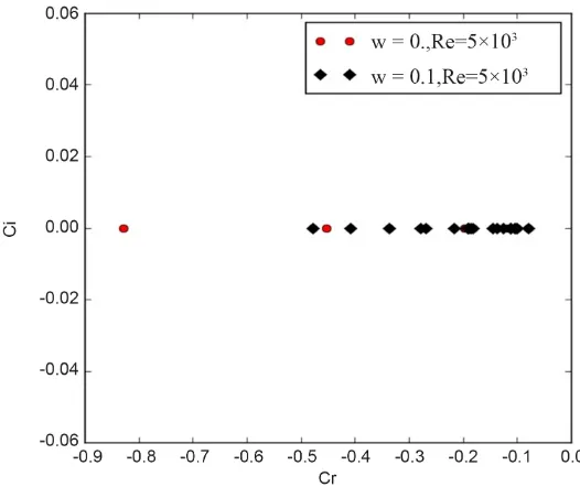
5.1. Case of One-Dimensional Disturbance (

n

= 0;

l

= 0)

Let us first note that for such a flow, the radial component of the velocity is zero

(

u=0

)

. On the other hand, the Figure 1 clearly shows that the fluid is Newto-nian

(

ω

=0

)

_{or viscoelastic}

(

ω

>0

)

_{, the eigenvalues are purely real and}

nega-tive that it’s worth the Reynolds’ number Re. For both types of fluid, the flow re-mains stable whatever the Reynolds number.

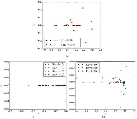
5.2. Case of Homogeneous Disturbance (

n

≠ 0;

k

0

= 0)

The eigenvalues related to this flow are real and negative for the case of the Newtonian fluid. The result does not change when increasing the number of Reynolds up to values close to 107₍_{Figure 2(b)}_{). On the other hand, this is not}

always the case for a viscoelastic fluid. For this type of fluid the real part of some eigenvalues is positive for even for a Reynolds number equal to _{5 10}3

e

R = × _.

However, instability occurs with a higher Reynolds number when the Weissen-berg’s number We decreases (Figure 2(c)). The flow of a Newtonian fluid is sta-ble whereas that of a viscoelastic fluid is unstasta-ble for a Reynolds number ( _{5 10}3

e

R = × _).

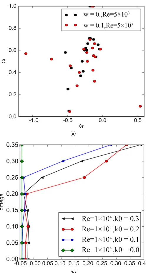
5.3. Case of an Axisymmetric Disturbance (

n

= 0;

k

0

≠

0)

[image:8.595.241.504.452.673.2]

The real parts of the eigenvalues remain negative for the Newtonian fluids, whe-reas for the same flow conditions, the real parts of the eigenvalues are not all negative for a viscoelastic fluid, which testifies to the appearance of instabilities in flow. It is also noted that beyond a certain value of the Reynolds number, in-stabilities appear in the flow itself for the Newtonian fluid, which is not the case

Figure 1. Spectrum of the eigenvalues of a one-dimensional disturbance

(

n=0,k0=0

)

,

case of Newtonian fluid (in red), case of viscoelastic fluid (black), with Reynolds’ number

3

5 10 e

(9)

DOI: 10.4236/mme.2018.84018 272 Modern Mechanical Engineering (a)

[image:9.595.64.539.71.484.2]

(b) (c)

Figure 2. (a) Spectrum of the eigenvalues of a homogeneous disturbance along the axis with n=1;k0=0, case of a Newtonian

fluid (black), case of a viscoelastic fluid (red) with Reynolds number _{5 10}3

e

R = × and Weissenberg’s number _We₌₁₀−2_{; (b)}

Spectrum of the eigenvalues of a homogeneous disturbance along the axis with for different values of the Reynolds number: case of a Newtonian fluid

(

ω =0

)

; (c) Spectrum of the eigenvalues of a homogeneous disturbance along the axis with n=1;k0=0 for

different values of the Reynolds number: case of a viscoelastic fluid with _We₌₁₀−3

.

for one-dimensional and homogeneous flows. Indeed, the term convection

(

u⋅ ∇

)

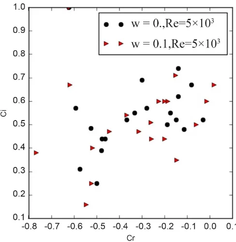
u, responsible for the exchanges between the base flow and the disturbed flow, is a source of instabilities, a term which is also nil for the Newtonian one-dimensional and homogeneous flows. In addition, it is noted (Figure 3(b)) that the greater the elasticity of the fluid, the greater the instability is important. From this it can be deduced that elasticity is also a source of instability.

5.4. Case of Three-Dimensional Perturbation (

n

≠ 0;

l

≠ 0)

(10)

DOI: 10.4236/mme.2018.84018 273 Modern Mechanical Engineering (a)

[image:10.595.248.496.69.531.2]

(b)

Figure 3. (a) Spectrum of the eigenvalues of an axisymmetric disturbance with

0

0; 0.1

n= k = , case of the Newtonian fluid (black), case of the viscoelastic fluid (red) with

3

5 10 e

R = × and _We₌₁₀−2_{; (b) Evolution of the most unstable eigenvalue according to}

the delay parameter ω with Reynolds’ number _Re₌₁₀4_{and Weissenberg’s number} 2

10

We₌ − _{; (b) shows that the one-dimensional flow of a viscoelastic fluid with a Reynolds} number _Re₌₁₀4_{is stable for a delay parameter ranging from 0 (Newtonian fluid) to}

0.35. The homogeneous flow of a viscoelastic fluid remains stable as long as the retarda-tion parameter is less than 0.2 and then becomes unstable beyond this value, but this flow remains stable until ω=0.25 for k0=0.1. However at beyond k0=0.1, this

thre-shold of instability is reached from ω=0.2.

the eigenvalues are not negative and would indicate that the fluid flows unstable for the same Reynolds number _{5 10}3

e

(11)

[image:11.595.249.493.71.321.2]

Figure 4. Spectrum of the eigenvalues of a three-dimensional perturbation n=1;k0=0.1

case of the Newtonian fluid (black), case of viscoelastic fluid (red) with Reynolds number

3

5 10

Re= × _{and Weissenberg’s number}_We₌₁₀−2_.

6. Conclusion

The analysis of the different results shows that the linear flow of a Newtonian fluid is stable, whereas that of a viscoelastic fluid with a number of Weissenberg

2

10

We₌ − _{and for a delay parameter (}_ω₌_0.1_{) is unstable at from} _{5 10}3

e

R = ×

except for the one-dimensional case. Indeed, for the one-dimensional and ho-mogenous cases, the term relating to the convection which is responsible for the exchange of energies between the base flow and the disturbed flow is almost nil. It can therefore be said that viscoelasticity and the term convection are at the origin of the instabilities observed.

Conflicts of Interest

The authors declare no conflicts of interest regarding the publication of this pa-per.

References

[1] Meseguer, A. and Trefethen, L.N. (2003) Linearized Pipe Flow to Reynolds Number 107_._Journal_of_{Computational}_Physics_{, 186, 178-197.}

https://doi.org/10.1016/S0021-9991(03)00029-9

[2] Esmael, A. (2008) Transition to Turbulence for a Flow through Fluid in a Cylin-drical Pipe. PhD thesis, INPL, Nancy.

[3] Carranza, L. (2012) Laminar-Turbulent Transition in Cylindrical Pipe for a Non-Newtonian Fluid. PhD Thesis, INPL, Nancy.

(12)

Pro-DOI: 10.4236/mme.2018.84018 275 Modern Mechanical Engineering

ceedingsoftheRoyalSocietyA, 200, 523-541.

https://doi.org/10.1098/rspa.1950.0035

[5] Bergstrom, L. and Brosa, U. (1988) Onset of Turbulence in a Pipe. Zeitschrift für Naturforschung, 43a, 696.

[6] Komminaho, J. and Johansson, A.V. (2000) Development of a Spectrally Accurate DNS Code for Cylindrical Geometries, Part V of J. Komminaho, Direct Numerical Simulation of Turbulent Flow in Plane and Cylindrical Geometries. Docoral Thesis, Royal Institute of Technology, Stockholm.

[7] Zhang, Y., Gandhi, A., Tomboulides, A.G. and Orzag, S.A. (1994) Simulation of Pipe Flow. In: Application of Direct and Large Eddy Simulation to Transition and Turbulence, AGARD Conference, Crete, 17.1-17.9.

[8] Zikanov, O.Yu. (1996) On the Instability of Pipe Poiseuille Flow. Physics of Fluids, 8, 2923. https://doi.org/10.1063/1.869071

[9] Bergstrom, L. (1997) Optimal Growth of Small Disturbances in Pipe Poiseuille Flow. Physics of Fluids, 9, 1043.

[10] Leonard, A. and Wray, A. (1982) A New Numerical Method for the Simulation of Three-Dimensional Flow in a Pipe. In: Krause, E., Ed., Proceedings of the 8th In-ternational Conference on Numerical Methods in Fluid Dynamics onNumerical MethodsinFluidDynamics, Springer, Berlin, 335-342.

https://doi.org/10.1007/3-540-11948-5_40

[11] Schmid, P.J. and Henningson, D.S. (1994) Optimal Energy Grothin Hagen-Poiseuille Flow. Journal of Fluid Mechanics, 277, 197.

https://doi.org/10.1017/S0022112094002739

[12] Trefethen, A.E., Trefethen, L.N. and Schmid, P.J. (1999) Spectra and Pseudospectra for pipe Poiseuille Flow. Computer Methods in Applied Mechanics and Engineer-ing, 175, 413-420. https://doi.org/10.1016/S0045-7825(98)00364-8

[13] Chupin, L. (2003) Contribution to the Study of Mixtures of Viscoelastic Fluids. Doctoral Thesis, The Mathematical Institute of Bordeaux, 177 p.

[14] Meseguer, A. and Trefethen, L.N. (2001) A Spectral Petrov-Galerkin Formulation for Pipe Flow II: Nonlinear Transitional Stages. Numerical Analysis Group, Oxford University, Rep. 01/19.

[15] Meseguer, A. and Trefethen, L.N. (2000) A Spectral Petrov-Galerkin Formulation for Pipe Flow (I): Linear Stability and Transient Growth. Numerical Analysis Group, Computing Lab, Oxford University, Rep. 00/18.

[16] Meseguer, A. and Mellibovsky, F. (2007) On a solenoidal Fourier-Chebyshev Spec-tral Method for Stability Analysis of the Hagen-Poiseuille Flow. AppliedNumerical Mathematics, 57, 920-938. https://doi.org/10.1016/j.apnum.2006.09.002

[17] Berlioz, J.P. (1979) A propos de l’algorithme QZ. RAIRO-AnalyseNumérique, 13, 21-30. https://doi.org/10.1051/m2an/1979130100211

[18] Quarteroni, A., Sacco, R. and Saleri, F. (2004) Méthodes Numériques: Algorithmes, analyse et applications. Springer-Verlag, Italia, Milano.

(13)

Appendix Code

The algorithm QZ makes possible to determine the eigenvalues and optionally the eigenvectors of the problem with generalized eigenvalues

(

Av=χBv

)

. The idea is to transform the matrices A and B into similar upper triangular matrices. If A and B

are respectively upper hessenberg and triangular matrices respectively. We call the QZ decomposition of pair

(

A B,

)

, the double factorization 

_{( )}

QA R_{QB Z T}= ₌

 with Q

unitary matrix, Z upper Hessenberg, R and T upper triangular. We will note later on

QAZ A QBZ B

 =

 

= 



 we can construct a unitary decomposing matrix A, as a product of

1

n− matrices of elementary rotation: _{Q Q}₌ (n−1) _{Q Q}( ) ( )2 1

 where each _Q( )i _is

a complex rotation matrix. _Q( )i _{modifies the first and second lines of}_B_possibly

creating a non-zero element in position

( )

2,1 which will have to be cancelled by a complex rotation matrix Z1 modifying only the first and the second col-umn of _{Q B}( )1 _{. Note} _B( )1 ₌_B_and _B( )2 ₌_{Q B Z}( ) ( ) ( )1 1 1 _.

( )2

B is triangular superior.

Let _B( )k _{be the upper triangular, let} _Q( )k _{be the rotation matrix modifying}

only the kth and (k + 1)th row of _B( )k _{possibly creating a non-zero element in}

position

(

k+1,k

)

_{which will have to be canceled by a matrix complex rotation}

( )k

Z only modifying the kth and (k + 1)th columns of _{Q B}( ) ( )k k _.

Let’s say _B(k+1)_{is upper triangular, the process stops for}_{k n}_{= −}₁_{and we} can write_{B QBZ B}_₌ ₌ ( )n _, _{Z Z}₌ ( )1 _×_Z( )2 _{× ×}_Z( )n−1

 .

If B is invertible, it is obvious that Q realizes a unitary and triangular decom-position of _AB−1_and _Z*_{a unitary decomposition of} _{B A}−1 _{, in fact:}

* 1 * 1 *

Z B A Z B Q QA BQA− ₌ − ₌ 

(14)

Nomenclature

Greek letters

θ: Azimuthal coordinate

λ: Relaxation time of the fluid

λ′_{: delay time}

ν: Kinematic viscosity of the fluid

ρ: Density of the fluid

σ: Tensor of extra stress

σ′_{: Disturbance of extra-stress} s

σ : Newtonian contribution of the disturbance of the extra-stress

e

σ : Elastic contribution of the disturbance of the extra-stress

η: Dynamic viscosity of the fluid

ϕ: Basis function

ψ: Test function

ω: delay parameter

Latin letters

Ci: imaginary part of the eigenvalue

Cr: real part of the eigenvalue

f: density force

l: axial mode

k0: Axial wave number

n: Azimuthal mode

r: radial coordinate

R: radius of the cylinder

Re: Reynolds number

W0: Maximum speed of the base flow, it has for direction that of the axis of the cylinder

We: Weissenberg’s number

Wb: Axial velocity of the base flow

s b

W : Newtonian contribution of basic flow velocity

e b

W : Elastic contribution of basic flow velocity