Multilayer Hex-Cells: A New Class of Hex-Cell
Interconnection Networks for Massively Parallel Systems
Mohammad Qatawneh
Computer Science Department, University of Jordan, Amman, Jordan E-mail: [email protected]
Received September 22, 2011; revised October 13, 2011; accepted November 10, 2011
Abstract
Scalability is an important issue in the design of interconnection networks for massively parallel systems. In this paper a scalable class of interconnection network of Hex-Cell for massively parallel systems is intro-duced. It is called Multilayer Hex-Cell (MLH). A node addressing scheme and routing algorithm are also presented and discussed. An interesting feature of the proposed MLH is that it maintains a constant network degree regardless of the increase in the network size degree which facilitates modularity in building blocks of scalable systems. The new addressing node scheme makes the proposed routing algorithm simple and ef-ficient in terms of that it needs a minimum number of calculations to reach the destination node. Moreover, the diameter of the proposed MLH is less than Hex-Cell network.
Keywords: Multilayer Hex-Cell, Interconnection Network, Parallel System
1. Introduction
The interconnection network strongly affects the per-formance of parallel machines. Many interconnection networks were proposed, from theslow but inexpensive single bus, to the extremely fast and very expensive cross-bar network [1-4]. In an interconnection network, degree related to hardware cost and diameter related to massage passing time is correlated with each other. In general, as degree of an interconnection network is in-creased, diameter is dein-creased, which can increase throughput in the interconnection network, however, it increases hardware cost with the increased number of links of the processors when parallel system is designed [2,5-7].
Among the wide variety of interconnection networks structures proposed for parallel computing systems is hex-cell which received much attention due to the attrac-tive properties such as embeddability and simple routing [8]. However, in an identical hex-cell network the di-ameter increases with the increase of the network size, which can decrease throughput of the network. Ideally, we would like to construct a new network that combines features such as less communication, efficient routing and capability of embedding other static topologies. This gives the motivation to develop a new interconnection network to meet the demands of highly parallel systems.
In this paper, a new interconnection network called Multilayer Hex-Cells network (MLH), which requires less diameter than a comparable size hex-cell network and with a constant network degree, is proposed. An-other advantage of the MLH network is that it is hierar-chical network, which makes it suitable for the connec-tionist models of computations, which requires a very large number of processors and its applications are hier-archical in nature. This paper concentrates on a network that enjoys the same ease of routing as in the hex-cell network.
The organization of this paper is as follows. Section 2 describes the definition of Hex-Cell network. Section 3 introduces the proposed Multilayer Hex-Cell network. Section 4 presents the routing algorithm of MLH and Section 5 summarizes and concludes the paper.
2. Definition of Hex-Cell Network
d
shown in Figure 1. Each level i has Ninodes, where Ni
= 6(2i – 1) and the total number of nodes in a Hex-Cell network HC(d) is N = 6d2. Each node in the HC is identi-fied by a pair (X.Y), where X denotes the line number in which the node exists, and Y denotes the location of the node in the line as in Figure 2. A node with the address 1.1 is the first node that exists at line number 1. 1.2 refers to the second node that exists at line number 1, and so on.
3. Multilayer Hex-Cells Interconnection
Network
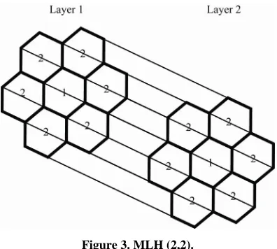
The Multilayer Hex-Cell (MLH) is a modular intercon-nection network that consists of layers of identical Hex-Cell networks connected together in a hierarchical fashion as shown in Figure 3. The MLH is denoted by MLH(k,d), where k denotes the layer number, and d de-notes the depth of the identical Hex-Cell. Each Layer k has Ni nodes, where Ni = 6d2 and the total number of
nodes in MHL network is 6 kd2. Lemma 1:
The total number of nodes in a MLH(k,d) with k layers is:
2
6 MLH
N k . (1)
Proof:
Using the previous definition of HC(d), it can be eas-ily seen that the total number of nodes at level 1 as shown in Figure 1 is N1 = 6 nodes, since there is a single
[image:2.595.325.523.76.254.2]Figure 1. (a) HC (one level); (b) HC (two levels); (c) HC (three levels).
Figure 2. Addressing nodes in HC.
Figure 3. MLH (2,2).
hexagon cell with six nodes. Level 2 introduces six hexagon cells (one at each side of the hexagon at level 1). It can be seen that level (i + 1) has 12 nodes in addition to corresponding nodes to those at level i. Therefore, the total number of nodes at level i is:
6 1 *12 6 2 1 i
N i i
(2)The total number of nodes in an identical Hex-Cell network HC(d) with d levels can be expresses as follows:
16 2 1d
h c i
N
i
(3)Therefore,
2 12 6 1 6 9 1 6 6
N
i
d d d d (4)The total number of nodes in MLH(k,d) with k layers can be expresses as follows:
2
6 MLH
N kd . (5)
3.1. Node Degree
[image:2.595.59.286.451.577.2] [image:2.595.61.286.619.704.2]3.2. Diameter
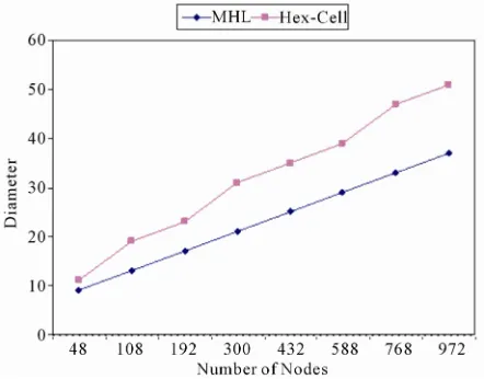
The diameter (D) of a network is the maximum shortest path between any two nodes. If the source and destina-tion nodes are located in the same layer (i.e. in the iden-tical HC(d) the diameter is equal to 4d – 1 [8], but if the source and destination nodes are located in different lay-ers in MLH(k,d), the number of k (layer) steps required to reach the destination node as shown in Case 1 and Case 2 in the proposed routing algorithm in the section 4. so the diameter of MLH(k,d) is 4d – 1 + k. Figure 4 shows, that the diameter against network size of the MLH is less than Hex-Cell network.
4. Proposed Routing Algorithm
In order to explain the following algorithm, we use the layer and line numbering scheme as follows. Each node in the MLH is identified by a pair (K.X.Y), where k de-notes the layer number, X denotes the line number in which the node exists, and Y denotes the location of the node in the line as in Figure 5. A node with the address 1.1.1 is the first node that exists at layer 1 and line num-ber 1. The Node1.1.2 refers to the second node that exists at layer and 1 and line number 1, and so on.
The proposed addressing node scheme can make the proposed routing algorithm simple and efficient in term of the number of operations needed to calculate the next node, especially when the source and destination nodes are located in different layers as discussed in the Exam-ples 1 and 2. The number of calculations is equal to n (n = the difference between the source and destination layer numbers).
[image:3.595.316.531.76.245.2]In the proposed routing algorithm for MLH as shown in Figure 6, the movement from one node to another node can be done by using one of the following three cases:
Figure 4. Diameter against the network size.
Figure 5. Addressing nodes in MLH(2,2).
moveUp(Ks,Xs,Ys, Kd, Xd,Yd)
if(Xs≠Xd)
if(Xs > depth)
if(Xs-1 = depth && Ys is odd) → moveUp(Ks,Xs-1,Ys, Kd, Xd Yd)
else if (Ys is even)
if (Ys > Yd) → moveUp (Ks,Xs,Ys-1, Kd, Xd Yd)
else → moveUp(Ks,Xs,Ys+1, Kd, Xd Yd)
else → moveUp(Ks,Xs-1,Ys+1, Kd, Xd Yd)
else if (Ys is odd)
if ( Ys > Yd)→ moveUp (Ks,Xs,Ys-1, Kd, Xd Yd)
else → moveUp(Ks,Xs,Ys+1, Kd, Xd Yd)
else→ moveUp(Ks,Xs-1,Ys-1, Kd, Xd Yd)
else if (Ys≠ Yd)→ moveHorizontal(Ks,Xs,Ys, Kd, Xd Yd)
else → Destination Reached
moveDown(Ks,Xs,Ys, Kd, Xd,Yd)
if(Xs≠Xd)
if(Xs > depth)
if (Ys is even) moveDown(Ks,Xs+1,Ys-1,Kd,Xd,Yd)
if (Ys > Yd) → moveDown (Ks,Xs,Ys-1, Kd, Xd Yd)
else → moveDown(Ks,Xs,Ys+1, Kd, Xd Yd)
else if (Ys is odd)
if (Xs < depth) moveDown((Ks,Xs+1,Ys+1,Kd,Xd,Yd)
else → moveDown(Ks,Xs+1,Ys, Kd, Xd Yd)
else→ (Ys > Yd) → moveUp(Ks,Xs,Ys-1,Kd,Xd,Yd)
else→ moveDown (Ks,Xs,Ys+1,Kd,Xd,Yd)
else if (Ys≠ Yd) → moveHorizontal(Ks,Xs,Ys,Kd,Xd,Yd)
else → Destination Reached
moveHorizontal (Ks,Xs,Ys, Kd, Xd,Yd)
if(Ys≠ Yd)
if(Ys> Yd) → moveHorizontal(Ks,Xs,Ys-1, Kd, Xd,Yd)
else → moveHorizontal(Ks,Xs,Ys+1, Kd, Xd,Yd)
[image:3.595.309.537.258.557.2]else→Destination Reached.
Figure 6. Routing algorithm for MLH(k,d).
CASE 1: If (Ks = Kd) & (Xs > Xd) then moveUp (Ks, Xs,
Ys, Kd, Xd, Yd)
else if (Ks= Kd) & (Xs < Xd) then moveDown(Ks, Xs, Ys,
Kd, Xd, Yd)
else if ((Ks = Kd) & (Xs = Xd) then moveHorizontal(Ks,
Xs, Ys, Kd, Xd, Yd).
CASE 2: If (Ks > Kd) then (Ks – 1, Xs, Ys, Kd, Xd, Yd).
CASE 3: If (Ks < Kd) then (Ks + 1, Xs, Ys, Kd, Xd, Yd).
where, Ks is the layer number of source node, Xs is the
line number of source node, and Ys is the location of
source node in line the number, Kdis the layer number of
[image:3.595.62.283.534.707.2]node, and Yd is the location of destination node in the
line number. One of the previous cases will be called recursively until the destination has been reached.
Discussions via Examples
The following examples explain the above routing cases. For this purposed, we consider a network of a MLH(2,2) as shown in Figure 7.
Example 1: If (Ks < Kd).
Let (1.1.4) and (2.2.5) be the address of the source and destination nodes respectively. CASE 3 of the routing algorithm (i.e. source layer + 1) and moveDown will use the following path: (2.1.4) → (2.1.5) → (2.2.5) as shown in Figure 6. From Example 1, it can be easily seen that, in order to forward a message to the next node, the rout- ing algorithm performs only one operation (subtraction) to the source layer (Ks – 1) and so on until the message
reaches its destination layer. When the source and desti- nation layers are equal, the routing algorithm forwards the message by applying the moveDown procedure as shown in the Figure 7.
Example 2: If (Ks> Kd).
Let (2.3.7) and (1.1.4) be the address of the source and destination nodes respectively. CASE 2 of the routing algorithm (i.e. source layer –1) and moveUp will use the following path: (1.3.7) → (1.2.7) → (1.2.6) → (1.1.5) →
(1.1.4) as shown in Figure 6. From Example 2, it can be easily seen that, in order to forward a message to the next node, the routing algorithm performs only one operation (addition operation) to the source layer (Ks + 1) and so on
until the message reaches its destination layer. When the source and destination layers are equal, the routing algo-rithm forwards the message by applying the moveUp procedure as shown in the Figure 7.
Example 3: If (Ks = Kd).
Let (1.4.5) and (1.4.1) be the address of the source and destination nodes respectively.
CASE 1 of the routing algorithm (i.e. Ks= Kd). From
the address of the source and destination nodes, it is clear that they are located at the same level (level 4). Applying the routing algorithm the moveHorizontal will be used.
Figure 7. MLH(2,2).
The move Horizontal procedure will use the following path: (1.4.4) → (1.4.3) → (1.4.2) → (1.4.1).
5. Conclusions
This paper introduced a new interconnection topology called Multilayer Hex-Cells. Additionally, the paper proposed an efficient routing algorithm for MLH which requires no detailed knowledge of the network. The new addressing node scheme makes the proposed routing algorithm simple and efficient in terms of that it needs a minimum number of calculations to reach the destination node. The proposed MLH maintains a constant network degree regardless of the increase in the network size de-gree which facilitates modularity in building blocks of scalable systems. Moreover, the diameter of the proposed MLH is less than Hex-Cell.
While the proposed topology has been analyzed ma- thematically and discussed through examples, it can be tested as an underlining network for many applications in distributed systems area.
6. References
[1] A. Mokhtar, “Multi-Level Hypercube Network,”
Pro-ceedings of the 5th International Conference in Parallel Processing Symposium, Anaheim, 30 April - 2 May 1991,
pp. 475-480.
[2] S. Huyn, O. Jae-Chul and L. Hyeong-Ok, “Multiple
Re-duced Hypercube (MRH): A New Interconnection Net-work Reducing Both Diameter and Edge of Hypercube,”
International Journal of Grid and Distributed Computing,
Vol. 3, No. 1, 2010, pp. 19-30.
[3] Y. Y. Liu and J. G. Han, “Double-Loop Hypercube: A
New Scalable Interconnection Network for Massively
Parallel Computing. Computing,” Proceedings of the
ISECS International Colloquium on Computing, Commu- nication, Control, and Management, Guangzhou, 3-4 Au-
gust 2008, pp. 170-174. doi:10.1109/CCCM.2008.45
[4] T. Chan and Y. Saad, “Multigrid Algorithms on the
Mul-tiprocessor,” IEEE Transactions on Computers, Vol. C-35, No. 11, 2002, pp. 969-977.
doi:10.1109/TC.1986.1676698
[5] S. Syed, K. Rizvi, M. Elleithy and A. Riasat, “An
Effi-cient Routing Algorithm for Mesh-Hypercube (M-H)
Networks,” Proceedings of the International Conference
on Parallel and Distributed Processing Techniques and Applications, Las Vegas, 14-17 July 2008, pp. 69-75.
[6] C. Decayeux and D. Seme, “3D Hexagonal Network:
Modeling, Topological Properties, Addressing Scheme,
and Optimal Routing Algorithm,” IEEE Transaction on
Parallel and Distributed Systems, Vol. 16, No. 9, 2005,
pp. 875-884. doi:10.1109/TPDS.2005.100
[7] K. Day and A. Al-Ayyoub, “Topological Properties of
Distributed Systems, Vol. 13, No. 4, 2002, pp. 359-366.
doi:10.1109/71.995816
[8] A. Sharieh, M. Qatawneh, W. Almobaideen and A. Sliet,
“Hex-Cell: Modeling, Topological Properties and
Rout-ing Algorithm,” European Journal of Scientific Research,