ISSN Online: 2160-0481 ISSN Print: 2160-0473
DOI: 10.4236/jtts.2019.91001 Nov. 8, 2019 1 Journal of Transportation Technologies
Estimating Elasticities for Freight Transport
Using a Network Model: An Applied
Methodological Framework
Bart Jourquin
Université Catholique de Louvain, Louvain School of Management (LSM), Center for Operations Research and Econometrics (CORE), Louvain-la-Neuve & Mons, Belgium
Abstract
This paper presents a general framework that can be used to estimate direct and cross elasticities for freight transport using a network model. This me-thodology combines operational research (network assignments in a geo-graphical information system) with more classical econometrics (multinomial logit choice models). The application of the method to a real-world case is il-lustrated by a simple model that relies on the generalized cost of transport as the only explanatory variable in the utility function. The methodological framework allows, however, for the implementation of more complex func-tions. Beside the generalized cost functions for road, rail and inland water-ways transport, the network model needs origin-destination matrixes and di-gitized networks. They are imported from ETIS Plus, a European transport policy information system. A set of direct and cross elasticities is presented. The estimated values are obtained using two methods: the first computes standard elasticities, while the second estimates arc elasticities. Figures are presented for Europe and for a large region around the Benelux countries, where more competition exists between the three modes of interest.
Keywords
Elasticity Estimations, Freight Transport, Network Model, Conditional Logit, Model Validation
1. Introduction
Elasticities are often used in the context of transport policy decisions, to estimate the impacts of a new infrastructure on traffic or on modal split for instance. Published multi-mode analyses of freight transport elasticities provide estimates How to cite this paper: Jourquin, B. (2019)
Estimating Elasticities for Freight Transport Using a Network Model: An Applied Me-thodological Framework. Journal of Trans-portation Technologies, 9, 1-13.
https://doi.org/10.4236/jtts.2019.91001
Received: September 19, 2018 Accepted: November 5, 2018 Published: November 8, 2018
Copyright © 2019 by author and Scientific Research Publishing Inc. This work is licensed under the Creative Commons Attribution International License (CC BY 4.0).
http://creativecommons.org/licenses/by/4.0/
DOI: 10.4236/jtts.2019.91001 2 Journal of Transportation Technologies that cover a wide range of values. This diversity of results occurs because of dif-ferences in methodologies and available data, and difdif-ferences between transport markets. Spatial scope and zoning may also affect estimates. These factors must be kept in mind for a fair understanding of the estimated elasticities, their ap-propriate use in further modeling, as well as benchmark references in further studies. It goes behind the scope of this paper to present an extensive review of the relevant literature, but a recent overview and in-depth discussion can be found in Beuthe et al. [1]. The methodology presented in this paper uses aggre-gate cross section data and considers a range of several commodities. Surpri-singly, the interest for the estimation of elasticities for freight transport seems to be unequal over the past 40 years. As shown in Table 4, several researches were conducted at the end of the 70’, beginning of the 80’. Another series of papers were published around 2010.
In this paper, the dataset provided by the ETIS Plus European project is ex-tensively used. Among other stuff, this database provides origin-destination (OD) matrixes for the 10 NSTR “chapters” (groups) of commodities, both at the NUTS-2 and NUTS-3 regional levels. It also provides digitized road, inland wa-terways (IWW) and railway networks.
In order to compute the generalized cost (GC) of transport for each mode, OD pair and group of commodities, the Nodus transportation modeling soft-ware (http://nodus.uclouvain.be, Jourquin and Beuthe [2]) is used. After a Box-Cox transformation (Box and Cox [3]), these costs are used as input for a conditional logit modal choice analysis.
Once calibrated, the models are validated (comparison of the results against observed data) at three different levels, similarly to what is described in Jourquin [4].
The calibrated model is further used to estimate a series of direct and cross elasticities, that are discussed and compared to other values presented in the li-terature.
Beside the fact that the results presented in this paper are obtained using ex-clusively open access data (the ETIS database) and open source and cross-platform software (Nodus, R, MariaDB…), the key contribution of this work is the flexibility of the described framework and the attention paid to the validation of the model.
2. Model Setup
To start with, a calibrated multimodal reference scenario must be set up, which is based on the demand, embedded in OD matrixes, and the generalized cost of transport for each mode that can be used to perform the transportation tasks (OD cells). Therefore, generalized cost functions and digitized networks are needed.
DOI: 10.4236/jtts.2019.91001 3 Journal of Transportation Technologies format and can thus easily be handled. The matrixes are available for the three transport modes of interest and contain data for 10 categories of commodities (NSTR main chapters).
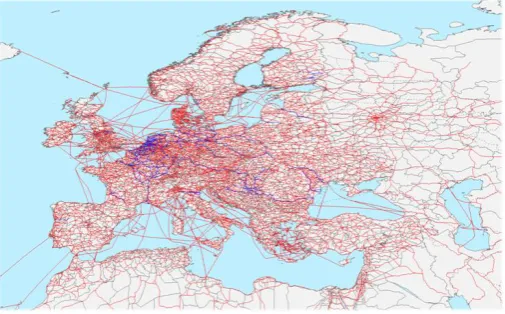
The digitized networks are available via a bulk download of the ETIS-NETTER data, in the ESRI shapefile format. Even if the downloaded files can be visualized directly in a GIS software, the networks cannot be used for as-signments. They are indeed not conceived for this, and some important mani-pulations are needed to make them “assignment compatible”. A description of the main operations to perform in order to obtain useable networks for trans-port assignment can be found in Jourquin [5]. The result is illustrated by Figure 1.
Generalized costs of transport are defined for each mode and each group of commodities. Obviously, it is not always possible to use the three transportation modes between every OD pair. Indeed, if road transport is generally possible, railways and, especially, inland waterways are not available everywhere. Nodus is useful here as it allows retrieving the GC of transport for each OD pair, each mode that can be used between O and D and each NST-R group of commodities for which a demand exists. The GC considers the costs of labor and capital, fuel, maintenance, …as explained in Beuthe et al. [1].
The loading and unloading costs ld and ul are fixed costs, while traveling cost mv depend on length L and speed S. The unit mv costs are defined for an aver-age speed S per mode. Thus, for a given link l belonging to a network of mode M, the moving cost is computed as:
M
l l M
l
mv S l C
S
= ∗ ∗ (1)
CM being the unit moving cost.
[image:3.595.248.501.547.704.2]As several types of vehicles m can sometimes be used on the links l of a modal network M (different types of barges on the IWW network for instance), and that the cost may differ for the different groups of commodities g, Equation (1) can be rewritten as:
DOI: 10.4236/jtts.2019.91001 4 Journal of Transportation Technologies
, ,
g m g
l m l m
l m
S
mv l C
S
= ∗ ∗ (2)
The generalized cost g m
GC of a route between an origin and a destination for a vehicle of type m transporting commodities of type g is thus equal to:
,
L
g g g g
m m m l m
l
GC =ld +ul +
∑
mv (3)where L is the set of successive links representing the route.
For the case presented in this paper, costs are defined for one type of truck and train, but for six types of barges (CEMT classes 2, 3, 4, 5a, 5b and 6). Note that all these barges cannot be used everywhere on the inland waterways net-work, as their usage is limited by the gage of the rivers.
The GC values are gathered from an assignment of the OD matrix on the digi-tized multimodal network. Thus, for each OD relation and each group of com-modities, a total generalized cost of transport is available for each mode that can be used, along with the total quantity (tonnage) to move. When several types of barges can be used on a relation, the one with the cheapest GC is retained for further use in the modal choice model.
These generalized costs of transport can further be used as explanatory varia-ble in a modal choice model. Classically (Ortúzar and Willumsen [6]), some kind of logit formulation can be used, but a few important characteristics must be considered:
As the generalized costs and, even more important, the spatial distribution of the demand and the supply are different for each group of commodities, spe-cific parameters should be estimated for each group.
The GC of transport is a choice (i.e. mode) specific, and not an individual
specific, variable. Therefore, a McFadden conditional logit (McFadden [7]) must be used. If g
m
U is the utility associated to a vehicle of mode m trans-porting goods of type g, the conditional logit formulation can be written as:
(
)
(
)
1
exp exp
g g
m g
m n g g
j j
U Pr
U
α α = =
∑
(4) where gm
Pr is the probability to choose mode m to transport commodity g, and n represents the number of modes in the choice set. The conditional logit differs from the multinomial logit as αg, the parameter to estimate, is not mode specific. As the model is solved separately for each group of commodities, this parameter varies, however, from group to group.
The OD matrix contains aggregated data. Indeed, each OD pair contains the
total transported tons per year for each mode and group of commodities, and not a specific transportation task. Hence, a weighted conditional logit must be estimated (Rich et al. [8]).
DOI: 10.4236/jtts.2019.91001 5 Journal of Transportation Technologies
(
)
g g g g
m m m
U =α −GC +δ (5)
g m
δ being an estimated intercept.
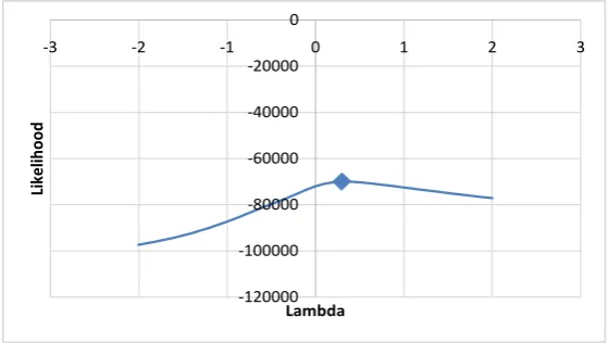
Note that, in order to maximize the likelihood of the estimated models, a Box-Cox (Box and Cox [3]) transformation can be applied to GC.
(
)
(
)
1, if 0 ,
log , if 0
g g
g m
g g
m
g g
m
GC B GC
GC
λ λ
λ λ
λ
− ≠
=
=
(6)
For each group of commodities g, a series of
λ
g values in the range [2,2]with a step of 0.1 are tested, and the value that maximizes the likelihood of the model is retained, as illustrated in Figure 2.
The utility function for each mode and group of commodities can thus be re-written as:
(
)
(
,)
g g g g g
m m m
U =α −B GC λ +δ (7)
Two models, based on different subsets of the ETIS Plus database, are esti-mated:
1) A model corresponding to the whole area covered by ETIS Plus (Figure 1, “Europe”).
2) The Benelux countries and their surrounding regions (“Benelux+”), inside which more competition between the three modes exists.
The
α
g and g mδ coefficients and the values of
λ
g are estimated using the“mnLogit” R package (Hasan et al. [9]), a faster and parallelized version of the well-known mLogit R package (Croissant [10]). All the estimated parameters all have the expected sign and are highly significant. This is true for all the groups of commodities in the two models.
3. Validation of the Models
The most straightforward way to check if a model fits is to compare the global estimated modal shares to the observed ones. To perform this check, the modal choice model (McFadden conditional logit with the estimated parameters) is ap-plied to the “merged” OD matrix1 and the resulting market shares are compared to those obtained from the three modal matrixes (before the merge). It comes out that, for both models, the estimated global market shares are equal to the observed ones for the three modes.
However, even if the estimated and observed market shares are identical, these figures are average values, and correct global market shares could very well be estimated while huge estimation errors are observed at the OD cell level. Further validation is therefore needed.
Once the modal choice model applied, the observed and estimated quantity transported by mode m between each origin O, destination D and for each
DOI: 10.4236/jtts.2019.91001 6 Journal of Transportation Technologies Figure 2. Example of best lambda identification (Europe, NSTR-3).
group of commodities g is available. This dataset can be used to compute a series of correlation coefficients r, given by Table 1.
It appears that, given the fact that the generalized cost of transport is the only explanatory variable used in the modal choice analysis, the model performs rea-sonably well when r is computed at the aggregated level (all modes together), but that it is sometimes much lower when computed for a single mode. This is par-ticularly the case for inland waterways transport in the European model. This is most probably linked to the fact that this mode is available in a few regions only. It is, for instance, much more present in the Benelux+ area, for which the cor-responding r value is noticeably higher.
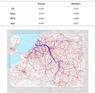
These first two validations are performed at the demand (node) level, but the network topology is still completely ignored. As no observed count data is avail-able along the segments of the networks, one could consider the results of the modal assignments (the OD matrix for a mode assigned to its own network) as a proxy. The correlation between the flow on some links2 resulting from these as-signments and the flow assigned to the same links by the multimodal model can be computed. The corresponding r values are published in Table 2 and show that, even with a simple univariate modal choice model using only generalized costs, the correspondence of the estimated flows on the networks with the “ob-servations” is more than satisfactory, the lowest value of r being 0.84.
Figure 3 illustrates the calibrated multimodal assignment for the Benelux+ region, which will be further used as input for elasticity estimations.
4. Estimating Elasticities
4.1. Methodology
The values of the direct and cross elasticities can be derived from the formula-tion of a McFadden condiformula-tional logit. With GC as the only explanatory variable, this logit specification can be written as:
-120000 -100000 -80000 -60000 -40000 -20000 0
-3 -2 -1 0 1 2 3
Lik
elih
oo
d
Lambda
2In order not to bias the correlation coefficient, links that are connected to two other links of the
DOI: 10.4236/jtts.2019.91001 7 Journal of Transportation Technologies Table 1. r values at the OD level.
Europe Benelux+
All 0.882 0.787
Road 0.932 0.864
IWW 0.570 0.726
Rail 0.841 0.767
Table 2. r values at the link level.
Europe Benelux+
All 0.943 0.912
Road 0.976 0.940
IWW 0.839 0.868
Rail 0.947 0.871
Figure 3. Calibrated assignment for the Benelux + region.
(
)
(
)
1
exp exp
g g
m g
m n g g
j j
GC Pr
GC
α α =
⋅ ⋅ =
∑
(8) The probabilities to choose mode/means m and mode/means j when com-modities of group g must be transported can be used to compute:(
)
ln mg g g g
m j
g j
Pr GC GC
Pr
α
= −
⋅ (9) Thus,
( )
2g
g g g g
m
m m
g m
Pr Pr Pr
GC α ⋅ α
∂
= −
[image:7.595.208.538.205.527.2]DOI: 10.4236/jtts.2019.91001 8 Journal of Transportation Technologies From which the direct elasticity can be derived as:
(
1)
g g
g g g
m m
m m
g g
m m
Pr GC GC Pr
GC ⋅ Pr α ⋅ ⋅
∂
= −
∂ (11)
Similarly,
0 g
g g g
m
m j
g j
Pr Pr Pr
GC α
∂
= − ⋅ ⋅
∂ (12)
From which the cross elasticity can be derived as:
g g
j g g g
m
j j
g g
j m
GC
Pr GC Pr
GC Pr
α
∂ ⋅ = − ⋅ ⋅
∂ (13)
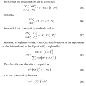
However, as explained earlier, a Box-Cox transformation of the explanatory variable is introduced, so that Equation (8) is replaced by:
(
)
(
)
(
)
(
)
1 exp exp g g m g m n g g j j GC Pr GC λ λ α α = ⋅ = ⋅∑
(14)Therefore, the own elasticity is computed as:
(
) (
1)
g g g
m m
GC λ Pr
α
⋅ ⋅ − (15)And the cross elasticity becomes:
(
)
g g g
j j
GC λ Pr
α
⋅− ⋅ (16)
Beside these standard elasticities, it is also possible to use Nodus to compute arc elasticities. Indeed, once the model calibrated, one just has to modify the transportation costs for one of the modes before running a new modal choice/assignment procedure. The elasticities can then be computed from the quantities Q assigned to each mode before (1) and after (2) the cost modifica-tion: 1 2 , 1 2 ln ln ln ln g g
g m m
m j g g
j j
Q Q
GC GC
ε = −
− (17)
Such arc elasticities3 computed with the network model offer more flexibility as it is easy to modify the total generalized cost or only one of its components. For instance, when the speed on the network links for a mode is modified, the influence of a change of travel time in GC can be estimated.
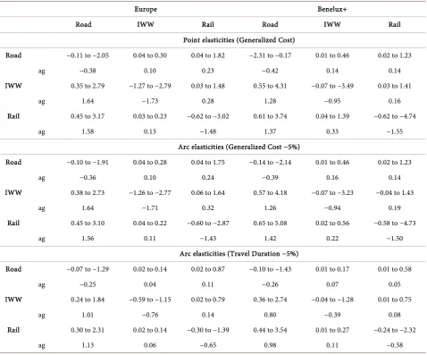
[image:8.595.201.546.73.417.2]4.2. Computed Elasticities
Table 3 summarizes the estimated elasticities. For each model, the standard and arc elasticities on GC and the arc elasticities when travel speed is changed on the networks are presented. Both the extreme values and the aggregated (all the groups of commodities together, “ag”) are published.
3The use of logarithms is not mandatory. They are used here in order to remain in line with the
DOI: 10.4236/jtts.2019.91001 9 Journal of Transportation Technologies Table 3. Set of estimated elasticities (Univariate Box-Cox Conditional logit model).
Europe Benelux+
Road IWW Rail Road IWW Rail
Point elasticities (Generalized Cost)
Road −0.11 to −2.05 0.04 to 0.30 0.04 to 1.82 −2.31 to −0.17 0.01 to 0.46 0.02 to 1.23
ag −0.38 0.10 0.23 −0.42 0.14 0.14
IWW 0.35 to 2.79 −1.27 to −2.79 0.03 to 1.48 0.55 to 4.31 −0.07 to −3.49 0.03 to 1.41
ag 1.64 −1.73 0.28 1.28 −0.95 0.16
Rail 0.45 to 3.17 0.03 to 0.23 −0.62 to −3.02 0.61 to 3.74 0.04 to 1.39 −0.62 to −4.74
ag 1.58 0.13 −1.48 1.37 0.33 −1.55
Arc elasticities (Generalized Cost −5%)
Road −0.10 to −1.91 0.04 to 0.28 0.04 to 1.75 −0.14 to −2.14 0.01 to 0.46 0.02 to 1.23
ag −0.36 0.10 0.24 −0.39 0.16 0.14
IWW 0.38 to 2.73 −1.26 to −2.77 0.06 to 1.64 0.57 to 4.18 −0.07 to −3.23 −0.04 to 1.43
ag 1.64 −1.71 0.32 1.26 −0.94 0.19
Rail 0.45 to 3.10 0.04 to 0.22 −0.60 to −2.87 0.65 to 5.08 0.02 to 0.56 −0.58 to −4.73
ag 1.56 0.11 −1.43 1.42 0.22 −1.50
Arc elasticities (Travel Duration −5%)
Road −0.07 to −1.29 0.02 to 0.14 0.02 to 0.87 −0.10 to −1.43 0.01 to 0.17 0.01 to 0.58
ag −0.25 0.04 0.11 −0.26 0.07 0.05
IWW 0.24 to 1.84 −0.59 to −1.15 0.02 to 0.79 0.36 to 2.74 −0.04 to −1.28 0.01 to 0.75
ag 1.01 −0.76 0.14 0.80 −0.39 0.08
Rail 0.30 to 2.31 0.02 to 0.14 −0.30 to −1.39 0.44 to 3.54 0.01 to 0.27 −0.24 to −2.32
ag 1.13 0.06 −0.65 0.98 0.11 −0.58
A few lessons can be drawn from this table. Firstly, the methods used to com-pute standard and arc elasticities result in almost the same figures. This is inter-esting, meaning that, using a network transport model, it is easy to measure the impact of a change of any variable composing of the generalized cost. This is il-lustrated in this paper by a change in travel time (speed on the links for a mode increased by 5%).
The range of estimated values is sometimes large among groups of commodi-ties. For instance, the direct GC elasticity for truck transport in the Benelux+ scenario varies from −2.31 to −0.17. However, the aggregated elasticity in this case is −0.42, indicating that the “extreme” values are obtained for categories of goods that are less representative. In this particular case, the −2.14 value is ob-tained for NSTR-2 (solid fuel), which represent only 1% of the total transported volume by road in the scenario. In all the cases, the aggregate elasticities are little affected by the extreme values.
DOI: 10.4236/jtts.2019.91001 10 Journal of Transportation Technologies the networks, one of the components of the generalized cost of transport. They are thus not the result of a specific modal choice model in which travel time is the/an explanatory variable. This being said, it comes out that the “travel time” elasticities represent roughly 50% of the values of the total generalized cost elas-ticities.
Finally, it is interesting to compare the cost elasticities presented in Table 3 with other values found in the literature. As outlined in the introduction, the di-versity of published values occurs because of differences in methodologies and available data, and differences between transport markets. Spatial scope and zoning may also affect estimates. These factors must be kept in mind for a fair understanding of the estimated elasticities, their appropriate use in further mod-eling, as well as benchmark references in further studies. Table 4 synthesizes the published estimates when aggregate cross section data and a range of several commodities are considered.
5. Conclusions
This paper presents a general methodology is able to obtain elasticity estimates for freight transport using a network model. Compared to similar approaches presented in the literature (Beuthe et al. [2] for instance), the presented method offers much more flexibility, as the modal choice model and the specification of the used utility function can be tailored. A special attention is also paid to the ca-libration and the validation of the model.
[image:10.595.208.537.500.741.2]The case that illustrates the method is based on a weighted conditional logit model, with a univariate utility function. A refinement is introduced as a Box-Cox transformation of the chosen explanatory variable (the generalized cost of transport) is used.
Table 4. Multi-modes direct price/cost elasticities (cross section).
Road IWW Rail
Levin (1978) [11] − − −0.25 to −0.35
Oum (1979) [12] −0.41 to −1.07 − −0.46 to −1.20 Friedlander and Spady (1980) [13] −0.14 to −1.72 − −1.45 to −4.01 Friedlander and Spady (1981) [14] −0.83 to −1.81 − −0.37 to −1.16 Kim (1987) [15] −0.10 to −1.24 − −0.12 to −1.73
Oum (1989) [16] −0.69 − −0.60
Beuthe et al. (2001) [17] 0.00 to −3.61 −0.04 to −10.5 −0.06 to −4.42 de Jong (2003) [18] −0.40 to −1.01 − −1.40 to −3.87 Rich et al. (2011) [19] −0.01 to −0.13 − −0.10 to −0.40 Beuthe et al. (2014) [1] −0.01 to −0.83 −0.39 to −0.99 −0.54 to −1.00 This paper (Benelux+) −2.31 to −0.17 −0.07 to −3.49 −0.62 to −4.74
DOI: 10.4236/jtts.2019.91001 11 Journal of Transportation Technologies The way elasticities can directly be derived from the logit model is explained, along with a method that estimates arc elasticities from a network model. The flexibility of the latest method is also demonstrated as elasticities can be esti-mated while only one component of the generalized costs is modified.
A set of elasticities is presented and compared to other values found in the li-terature.
This general framework opens the way to the use of more complex, multiva-riate utility functions, such as functions that combine (generalized) cost and transit time, which are often considered as the two most important drivers for a modal choice decision. Even if this bivariate approach sounds straightforward to apply, the important correlation between both variables cannot be underesti-mated, as is can lead to unexpected signs for the estimated parameters. This can be solved using Box-Cox transformations on both variables, with different lambdas. But this is another story...
Acknowledgements
I would like to thank my colleague Michel Beuthe for the stimulating discussions we had about the way to derive elasticity formulas from different logit model specifications.
Conflicts of Interest
The authors declare no conflicts of interest regarding the publication of this pa-per.
References
[1] Beuthe, M., Jourquin, B. and Urbain, N. (2014) Estimating Freight Transport Price Elasticity in Mode Studies: A Review and Additional Results from a Multi-modal Network Model. Transport Reviews, 34, 626-644.
https://doi.org/10.1080/01441647.2014.946459
[2] Jourquin, B. and Beuthe, M. (1996) Transportation Policy Analysis with a GIS: The Virtual Network of Freight Transportation in Europe. Transportation Research C, 4, 359-371. https://doi.org/10.1016/S0968-090X(96)00019-8
[3] Box, G. and Cox, D. (1964) An Analysis of Transformations. Journal of the Royal Statistical Society, Series B, 26, 211-252.
[4] Jourquin, B. (2016) Calibration and Validation of Strategic Freight Transportation Planning Models with Limited Information. Journal of Transportation Technolo-gies, 6, 239-256. https://doi.org/10.4236/jtts.2016.65023
[5] Jourquin, B. (2017) Estimation of Travel Time Elasticities with a Multimodal Freight Transport Model Calibrated and Validated on Publicly Available Regional Data. 14th International Nectar Conference, Madrid, 31 May-2 June 2017.
https://www.researchgate.net/publication/317580054_Estimation_of_travel_time_el
astici-ties_with_a_multimodal_freight_transport_model_calibrated_and_validated_on_p
ublicly_available_regional_data
DOI: 10.4236/jtts.2019.91001 12 Journal of Transportation Technologies [7] McFadden, D. (1973) Conditional Logit Analysis of Quantitative Choice Behavior.
In: Zarembka, P., Ed., Frontiers in Econometrics, Academic, New York.
[8] Rich, J., Holmblad, P. and Hansen, C. (2009) A Weighted Logit Freight Mode-Choice Model. Transportation Research Part E, 45, 1006-1019.
https://doi.org/10.1016/j.tre.2009.02.001
[9] Hasan, A., Zhiyu, W. and Mahani, A.S. (2016) Mnlogit: Multinomial Logit Model. R Package Version 1.2.5. https://cran.r-project.org/web/packages/mnlogit
[10] Croissant, Y. (2013) Mlogit: Multinomial Logit Models. R Package Version 0.2-4.
http://CRAN.R-project.org/package=mlogit
[11] Levin, R.C. (1978) Allocation in Surface Freight Transportation: Does Rate Regula-tion Matter? The Bell Journal of Economics, 9, 18-45.
https://doi.org/10.2307/3003610
[12] Oum, T.H. (1979) A Cross-Sectional Study of Freight Transport Demand and Rail-Truck Competition in Canada. The Bell Journal of Economics, 10, 463-482. https://doi.org/10.2307/3003347
[13] Friedlander, A. and Spady, R. (1980) A Derived Demand Function for Freight Transportation. The Review of Economics and Statistics, 62, 432-444.
https://doi.org/10.2307/1927111
[14] Friedlander, A. and Spady, R. (1981) Freight Transport Regulation: Equity, Effi-ciency and Competition. MIT Press, Cambridge, MA.
[15] Kim, B. (1987) The Optimal Demand for Freight Transportation in Strategic Logis-tics and Intermodal Substitution in the United States. Ph.D. Dissertation, Depart-ment of Economics, Northwestern University, Evanston Ill.
[16] Oum, T. (1989) Alternative Demand Models and Their Elasticity Estimates. Journal of Transport Economics and Policy, 23, 163-187.
[17] Beuthe, M., Jourquin, B., Geerts, J.-F. and Koul à Ndjang’ha, Ch. (2001) Freight Transportation Demand Elasticities: A Geographic Multimodal Transportation Network Analysis. Transportation Research Part E, 37, 253-266.
https://doi.org/10.1016/S1366-5545(00)00022-3
[18] de Jong, G. (2003) Elasticities and Policy Impacts in Freight Transport in Europe. European Transport Conference 2003, Strasbourg, 8-10 October 2003.
https://aetransport.org/en-gb/past-etc-papers/conference-papers-pre-2009/conferen
ce-papers-2003?abstractId=1566&state=b
DOI: 10.4236/jtts.2019.91001 13 Journal of Transportation Technologies
Symbols
C: Standard unit cost (per ton and kilometer for instance) GC: Generalized cost of transport
L: Set of successive links representing a route ld: Loading cost
mv: Moving cost Pr: Choice probability Q: Quantity to transport S: Speed
U: Utility function ul: Unloading cost
Indices
g: Group (category) of commodities l: Link (edge) ID in a network M: Transportation mode
m: Transportation means (type of vehicle within a mode) n: Available transportation modes
Parameters to Estimate
α: Coefficient to apply to a utility function (Logit model) δ: Intercept for a Logit model