GRAPHS OF TYPICAL CONTINUOUS FUNCTIONS
B. Adam-Day
e-mail: [email protected]
C. Ashcroft
e-mail: [email protected]
L. Olsen
Department of Mathematics University of St. Andrews St. Andrews, Fife KY16 9SS, Scotland
e-mail: [email protected]
N. Pinzani
e-mail: [email protected]
A. Rizzoli
e-mail: [email protected]
J. Rowe
e-mail: [email protected]
2000Mathematics Subject Classification.28A78, 28A80.
Key words and phrases: box dimension, continuous function, H¨older mean, Cesaro mean, Riesz-Hardy mean, Baire category.
Abstract. LetX be a bounded subset of Rd and write Cu(X) for the set of uniformly continuous functions on X equipped with the uniform norm. The lower and upper box dimensions, denoted by dimB(graph(f)) and dimB(graph(f)), of the graph graph(f) of a functionf∈Cu(X) are defined by
dimB(graph(f)) = lim inf
δ&0
logNδ(graph(f)) −logδ ,
dimB(graph(f)) = lim sup δ&0
logNδ(graph(f)) −logδ ,
whereNδ(graph(f)) denotes the number ofδ-mesh cubes that intersect graph(f). Hyde et al have recently proved that the box counting function
logNδ(graph(f))
−logδ (∗)
of the graph of a typical functionf∈Cu(X) diverges in the worst possible way asδ&0. More precisely, Hyde et al showed that for a typical functionf ∈ Cu(X), the lower box dimension of the graph off is as small as possible and ifX has only finitely many isolated points, then the upper box dimension of the graph off is as big as possible.
In this paper we will prove that the box counting function (∗) of the graph of a typical function
f ∈ Cu(X) is spectacularly more irregular than suggested by the result due to Hyde et al. Namely, we show the following surprising result: not only is the box counting function in (∗) divergent asδ&0, but it is so irregular that it remains spectacularly divergent asδ&0 even after being “averaged” or “smoothened out” using exceptionally powerful averaging methods includingallhigher order H¨older and Cesaro averages andallhigher order Riesz-Hardy logarithmic averages. For example, if the box dimension ofXexists, then we show that for a typical functionf ∈Cu(X),allthe higher order lower H¨older and Cesaro averages of the box counting function (∗) are as small as possible, namely, equal to the box dimension ofX, and if, in addition,X has only finitely many isolated points, thenallthe higher order upper H¨older and Cesaro averages of the box counting function (∗) are as big as possible, namely, equal to the box dimension ofX
plus 1.
1. Statements of the Main Results.
1.1. Introduction. Recall that in a metric space X, a set E is called co-meagre if its com-plement is meagre, and we say that a typical element x ∈ X has property P if the set E ={x ∈ X |xhas propertyP}is co-meagre, see Oxtoby [Ox] for more details.
For a bounded subsetXofRd, we letC
u(X) denote the set of uniformly continuous functions onX. It is well-known, and easy to see, that a uniformly continuous functionf :X→Ron a bounded subset X of Rd is bounded, and the spaceC
u(X) of uniformly continuous functions on X can be equipped with the uniform normk·k∞to form a normed space (Cu(X),k·k∞). It is well-known that the normed
space (Cu(X),k·k∞) is a Banach space, and below we will always equipCu(X) with the uniform norm.
We emphasise that the set X, except from being bounded, is completely arbitrary; for example, we are not assuming thatXis compact or Borel. Hyde et al [HyLaOlPeSh] have recently investigated the lower and the upper box dimension of the graph of a typical (in the sense of Baire) functionf ∈Cu(X). More precisely, Hyde et al [HyLaOlPeSh] proved that for a typical functionf ∈Cu(X), the lower box dimension of the graph off is as small as possible, namely, equal to the lower box dimension ofX, and ifX has only finitely many isolated points, then the upper box dimension of the graph off is as big as possible, namely, equal to the upper box dimension of X plus 1, see Theorem A below. The Hausdorff and packing dimensions of the graph of a typical continuous function f : [0,1]→ R
have also been studied by Mauldin & Williams [MaWi] and Humke & Petruska [HuPe], respectively. Indeed, Mauldin & Williams [MaWi] proved that the Hausdorff dimension of the graph of a typical continuous functionf : [0,1]→Ris as small as possible, namely, equal to 1, and Humke & Petruska
[HuPe] proved that the packing dimension of the graph of a typical continuous functionf : [0,1]→R
is as big as possible, namely, equal to 2. The purpose of this paper is to study this dichotomy in more detail. More precisely, we prove that the box dimension of the graph of a typical functionf ∈Cu(X) is spectacularly more irregular than suggested by the results in [HuPe,HyLaOlPeSh,MaWi]. However, we first recall that the box dimensions of a subset E of Euclidean space is defined as the lower and upper limits of the box counting function logNδ(E)
informal version of your main result. This result says, somewhat surprisingly, that the box counting function logNδ(graph(f))
−logδ of the graph graph(f) of a typical function f ∈Cu(X) is dramatically more irregular than suggested by the results in [HuPe,HyLaOlPeSh,MaWi].
Informal version of Theorems 1.1, 2.1 and 3.1. The box counting function
Λf(δ) = logNδ(graph(f))
−logδ (1.1)
of the graph graph(f) of a typical function f ∈ Cu(X) is so irregular that it remains spectacularly divergent as δ & 0 even after being “averaged” using very general and powerful averaging methods including higher order H¨older and Cesaro averages and higher order Riesz-Hardy logarithmic averages. For example, if we define then’th order H¨older averages, denoted byΛn
f(t), of the box counting function
in (1.1) inductively by
Λ0f(t) = Λf(e− t
), Λnf(t) =
1 t
Z t
1
Λnf−1(s)ds ,
forn∈Nandf ∈Cu([0,1]d), then a typical continuous functionf : [0,1]d→Rsatisfies
lim inf t→∞ Λ
n
f(t) =d , lim sup
t→∞
Λnf(t) =d+ 1,
for alln∈N∪ {0}.
1.2. Statement of the main results. We start by recalling the definition of the lower and upper box dimensions of subsets ofRm. Forδ >0, let
Qm δ =
( m
Y
i=1
[niδ,(ni+ 1)δ]
n1, . . . , nm∈Z
)
(1.2)
denote the standardδ-grid in Rm, and for a bounded subsetE of
Rmwrite
Nδ(E) =
n
Q∈ Qmδ
Q∩E6=∅ o
(1.3)
for the number of cubes inQm
δ that intersectE. The lower and upper box dimensions ofE are now defined by
dimB(E) = lim inf δ→0
logNδ(E)
−logδ , (1.4)
and
dimB(E) = lim sup δ→0
logNδ(E)
−logδ , (1.5)
respectively. If the lower and upper box dimensions of E coincide, then we will say that the box dimension ofE exists, and we will denote the common value by dimB(E), i.e. if dimB(E) = dimB(E), then we will write
dimB(E) = dimB(E) = dimB(E).
The reader is referred to Falconer [Fa] for a thorough discussion of the properties of the box dimensions. Forf ∈Cu(X), we will write graph(f) for the graph off, i.e.
graph(f) =n(x, f(x)) x∈X
o
.
Theorem A [HyLaOlPeSh]. Let X be a bounded subset of R.
(1) For all f ∈Cu(X), we have
dimB(X)≤dimB(graph(f))
≤dimB(graph(f))
≤ sup
ϕ∈Cu(X)
dimB(graph(ϕ))≤dimB(X) + 1.
(2) For a typical function f ∈Cu(X), we have
dimB(graph(f)) = dimB(X). (3) (i)For a typical functionf ∈Cu(X), we have
dimB(graph(f)) = sup ϕ∈Cu(X)
dimB(graph(ϕ))≤dimB(X) + 1.
(ii) If, in addition, X only has finitely many isolated points, then for a typical function f ∈
Cu(X), we have
dimB(graph(f)) = dimB(X) + 1.
Theorem A says that for a typicalf ∈Cu(X), the lower and upper box dimensions are as big and as small as they can be, respectively. In order to analyse this dichotomy in more detail, we introduce the following notation. Namely, for a bounded subset E of Rd, we define the box counting function
∆E : (0,∞)→[0,∞] ofE by
∆E(t) =logNe−t(E)
−loge−t =
logNe−t(E)
t . (1.6)
Then
dimB(E) = lim inf t→∞ ∆E(t)
and
dimB(E) = lim sup t→∞
∆E(t),
and Theorem A therefore shows that for typical f ∈ Cu(X), the box counting function ∆graph(f)(t)
of the graph of f diverges in the worst possible way ast→ ∞. In this paper we will prove that the behaviour of the box counting dimension function
t→∆graph(f)(t) =
logNe−t(graph(f))
t
of the graph of a typical functionf ∈Cu(X) is spectacularly more irregular than suggested by Theorem A. Namely, there are standard techniques, known as averaging methods, that (at least in some cases) can assign limiting values to divergent functions (the precise definitions will be given below), and the purpose of this paper is to show the following surprising result: not only is ∆graph(f)(t) divergent as
t → ∞, but the function ∆graph(f)(t) diverges so badly ast→ ∞, that even exceptionally powerful
averaging methods, including, for example, higher order H¨older and Cesaro averages and higher order Riesz-Hardy logarithmic averages, are not able to “smoothen out” the irregularities in ∆graph(f)(t) as
t→ ∞.
Definition. Average system. An averaging system is a familyΠ = (Πt)t≥t0 witht0>0such that:
(i) Πtis a finite Borel measure on [t0,∞);
(ii) Πthas compact support;
(iii) The Consistency Condition: Iff : [t0,∞)→[0,∞)is a positive measurable function and there
is a real number asuch that f(t)→aas t→ ∞, thenR
f dΠt→aast→ ∞.
Iff : [t0,∞)→[0,∞)is a positive measurable function, then we define lower and upperΠ-average of
f by
AΠf = lim inf t→∞
Z
f dΠt
and
AΠf = lim sup
t→∞ Z
f dΠt,
respectively.
The reader is referred to Hardy’s excellent classical text [Ha] for a detailed and thorough discussion of average systems, and examples that demonstrate when averaging methods do assign limiting values to divergent functions.
We will now apply various averaging methods to the box counting function ∆graph(f)(t) of f ∈
Cu(X). Namely, for a bounded subset E of Rm and a positive averaging method Π = (Πt)t
≥t0, we
define the lower and upper Π-average box dimensions ofE by dimΠ,B(E) =AΠ∆E
= lim inf t→∞
Z logN
e−s(E)
s dΠt(s),
and
dimΠ,B(E) =AΠ∆E
= lim sup t→∞
Z logN
e−s(E)
s dΠt(s),
respectively. The next statement, i.e. Theorem 1.1, is the main result in the paper. This result shows that the behaviour of a typical (in the sense of Baire category) function f ∈Cu(X) is so irregular that the box counting function t→∆graph(f)(t) of the graph off remains divergent ast → ∞even
after being “averaged” using very general and powerful averaging methods Π including, for example, higher order H¨older and Cesaro averages and higher order Riesz-Hardy logarithmic averages.
Theorem 1.1. Let Π = (Πt)t≥t0 be an averaging system and letX be a bounded subset ofR
d.
(1) For all f ∈Cu(X), we have
dimΠ,B(X)≤dimΠ,B(graph(f))
≤dimΠ,B(graph(f))
≤ sup
ϕ∈Cu(X)
dimΠ,B(graph(ϕ))≤dimΠ,B(X) + 1.
(2) For a typical function f ∈Cu(X), we have
dimΠ,B(graph(f)) = dimΠ,B(X). (3) (i)For a typical functionf ∈Cu(X), we have
dimΠ,B(graph(f)) = sup
ϕ∈Cu(X)
dimΠ,B(graph(ϕ))≤dimΠ,B(X) + 1.
(ii) If, in addition, X only has finitely many isolated points, then for a typical function f ∈
Cu(X), we have
The proof of Theorem 1.1 is given in Sections 5–8. Note that the statements in Theorem 1.1.(1) are trivial, and are merely included for completeness. Section 5 contains various preliminary results. The proof of Theorem 1.1.(2) is given in Section 6. The proof of Theorem 1.1.(3).(i) is given in Section 7, and the proof of Theorem 1.1.(3).(ii) is given in Section 8.
Remark. Note that if we let Π denote the average system defined by Π = (δt)t≥1 (whereδt denotes
the Dirac measure concentrated att), then
dimΠ,B(E) = dimB(E), dimΠ,B(E) = dimB(E),
for all subsetsEofRm. Hence, if we apply Theorem 1.1 to the average system defined by Π = (δt)t≥1,
then the statement in Theorem 1.1 simplifies to Theorem A.
If the box dimension ofX exists andX only has finitely many isolated points, then the statement in Theorem 1.1 simplifies considerably; this is the content of the next corollary.
Corollary 1.2. Let Π = (Πt)t≥t0 be an averaging system and let X be a bounded subset of R
d.
Assume that the box dimension of X exists and that X only has finitely many isolated points.
(1) For all f ∈Cu(X), we have
dimB(X)≤dimΠ,B(graph(f))≤dimΠ,B(graph(f))≤dimB(X) + 1.
(2) For a typical function f ∈Cu(X), we have
dimΠ,B(graph(f)) = dimB(X), dimΠ,B(graph(f)) = dimB(X) + 1.
In Sections 2–3, we present several applications of Theorem 1.1 to different averaging methods Π, namely:
• In Section 2 we apply Theorem 1.1 to H¨older and Cesaro averages. This allows us to compute the higher order H¨older and Cesaro averages of the box counting function ∆graph(f)(t) of a
typical functionf ∈Cu(X).
• In Section 3 we apply Theorem 1.1 to higher order Riesz-Hardy logarithmic averages. This allows us to compute the higher order Riesz-Hardy logarithmic averages of the box counting function ∆graph(f)(t) of a typical functionf ∈Cu(X).
2. H¨older and Cesaro averages of the box dimension of the graph of a typical function.
Two of the most commonly used averaging method are H¨older averages and Cesaro averages. We will now define these average methods and apply them to the box counting functiont→∆graph(f)(t)
of the graph off. We first recall the definitions of the H¨older and Cesaro averages. Fora >0 and a measurable functionf : (a,∞)→[0,∞), we defineM f : (a,∞)→[0,∞) by
(M f)(t) =1 t
Z t
a
f(s)ds .
For a positive integern, we now define the lower and uppern’th order H¨older averages off by Hnf = lim inf
t→∞ (M
nf)(t), Hnf = lim sup
t→∞
The Cesaro averages are defined as follows. First, we defineIf : (a,∞)→[0,∞) by
(If)(t) =
Z t
a
f(s)ds .
For a positive integern, we now define the lower and uppern’th order Cesaro averages off by Cnf = lim inf
t→∞
n! tn(I
nf)(t),
Cnf = lim sup t→∞
n! tn(I
n f)(t).
It is well-known that that the H¨older and Cesaro averages satisfy the following inequalities, namely, lim inf
t→∞ f(t) =H0f ≤H1f ≤H2f ≤. . .≤H2f ≤H1f ≤H0f = lim supt→∞ f(t),
lim inf
t→∞ f(t) =C0f ≤C1f ≤C2f ≤. . .≤C2f ≤C1f ≤C0f = lim supt→∞ f(t),
(2.1)
and
Cnf ≤Hnf ≤Hnf ≤Cnf . (2.2)
It is also well-known that the H¨older and Cesaro averages are averaging methods in the sense of the definition in Section 1.2. Indeed, if we for a positive integer n, define the averaging method ΠHn = (ΠHn,t)t≥a by
ΠHn,t(B) = 1 (n−1)!t
Z
[a,t]∩B
(logt−logs)n−1ds for Borel subsetsB of [a,∞), then
Hnf = lim inf t
Z
f dΠHn,t,
Hnf = lim sup t
Z
f dΠHn,t,
see, for example, [Ja, p. 675]. Similarly, if we for a positive integer n, define the averaging method ΠC
n= (ΠCn,t)t≥a by
ΠCn,t(B) = n tn
Z
[a,x]∩B
(t−s)n−1ds then
Cnf = lim inf t
Z
f dΠCn,t,
Cnf = lim sup t
Z
f dΠCn,t,
see, for example, [Ha, pp. 110-111]. For example, this shows that the n’th order lower H¨older and Cesaro averages off are given by
Hnf = lim inf t→∞
1 (n−1)!t
Z t
a
(logt−logs)n−1f(s)ds and
Cnf = lim inf t→∞
n tn
Z t
a
(t−s)n−1f(s)ds .
There are similar formulas for then’th order upper H¨older and Cesaro averages off.
Using H¨older and Cesaro averages we can now introduce average H¨older and Cesaro box dimensions by applying the definitions of the H¨older and Cesaro averages to the functiont→∆graph(f)(t). This
Definition. Average H¨older and Cesaro box dimensions. For a bounded subset E of Rm, we define the lower and uppern’th order average H¨older box dimension ofE, denoted bydimHB,n(E)and
dimHB,n(E), as the lower and uppern’th order H¨older average of the functiont→∆E(t)fort≥1, i.e.
we put
dimHB,n(E) =Hn∆E, dimHB,n(E) =Hn∆E.
Similarly, we define the lower and upper n’th order average Cesaro box dimension of E, denoted by
dimCB,n(E)anddimCB,n(E), by
dimCB,n(E) =Cn∆E, dimCB,n(E) =Cn∆E.
The higher order average H¨older and Cesaro box dimensions form a double infinite hierarchy in (at least) countably infnite many levels, namely, we have (using (2.1))
dimB(E) = dimHB,0(E)≤dimHB,1(E)≤. . .≤dimHB,1(E)≤dimHB,0(E) = dimB(E),
dimB(E) = dimCB,0(E)≤dimCB,1(E)≤. . .≤dimCB,1(E)≤dimCB,0(E) = dimB(E).
(2.3)
As an application of Theorem 1.1, we will now show that the behaviour of a typical functionf ∈Cu(X) is so irregular that not even the hierarchies in (2.3) formed by taking H¨older and Cesaro averages of all orders are sufficiently powerful to “smoothen out” the behaviour of the box counting function ∆graph(f)(t) ast→ ∞.
Theorem 2.1. Let X be a bounded subset of Rd with finitely many isolated points. Then a typical function f ∈Cu(X)satisfies:
dimHB,n(graph(f)) = dimHB,n(X), dimHB,n(graph(f)) = dimHB,n(X) + 1, dimCB,n(graph(f)) = dimCB,n(X), dimCB,n(graph(f)) = dim
C
B,n(X) + 1,
for alln∈N∪{0}. In particular, if, in addition, the box dimension ofX exists, then a typical function
f ∈Cu(X) satisfies:
dimHB,n(graph(f)) = dimCB,n(graph(f)) = dimB(X), dimHB,n(graph(f)) = dimCB,n(graph(f)) = dimB(X) + 1,
for alln∈N∪ {0}. Proof.
3. Riesz-Hardy averages of the box dimension of the graph of a typical function.
Higher order Riesz-Hardy logarithmic averages were introduced into the study of fractal properties of sets and measures by Fisher [Fi1] and Bedford & Fisher [BeFi] in the early 1990’s (see also [ArDeFi]), and has since been investigated further by a large number of authors, including Graf [Gr], M¨orters [M¨o1,M¨o2,M¨o3] and Z¨ahle [Z¨a]; the precise definition of the higher order Riesz-Hardy logarithmic averages will be given below. Motivated by this, we will now study the higher order Riesz-Hardy logarithmic averages of the box counting functiont→∆graph(f)(t) of the graph off. We first recall the
definition of higher order Riesz-Hardy logarithmic averages. Define log+:R→Rby log+(t) = log(t)
fort >0 and log+(t) = 0 fort≤0, and for a functionf :R→R, define the functionsEf, Lf :R→R
by
(Ef)(t) =f(et), (Lf)(t) =f(log+(t)).
Next, for a positive measurable functionf :R→[0,∞), we define the function Λf :R→Rby (Λf)(u) =e−u
Z u
−∞
etf(t)dt;
i.e. Λf is the convolution product betweenf and the functionλ:R→Rdefined byλ(t) = 0 fort≤0
andλ(t) =e−tfor 0< t. The higher order Riesz-Hardy logarithmic averages of a positive measurable functionf :R→[0,∞) are now defined as follows. Namely, for a positive integer n∈N, the lower
and uppern’th order Riesz-Hardy logarithmic averages are defined by Rnf = lim inf
t→∞ (L
nΛEnf)(t), Rnf = lim sup
t→∞
(LnΛEnf)(t).
It is well-known that that the Riesz-Hardy logarithmic averages satisfy the following inequalities, namely,
lim inf
t→∞ f(t) =R0f ≤R1f ≤R2f ≤. . .≤R2f ≤R1f ≤R0f = lim supt→∞
f(t) ; (2.4) the reader is referred to [BeFi, pp. 98–99, Property (1)] for a discussion of the proof of various special cases of (2.4), and note that [BeFi] refers the reader to [Fi2] for further discussions of the proof of (2.4) for an arbitrary positive measurable function f. It is also well-known that the Riesz-Hardy logarithmic averages are averaging methods in the sense of the definition in Section 1.2. Indeed, if we for a positive integern, define the averaging method ΠR
n= (ΠRn,t)t≥a fora >0 by ΠRn,t(B) = 1
logn+−1(t) Z
[a,t]∩B
logn+−1(s) n−1
Y
k=0
logk+(s) ds
for Borel subsetsB of [a,∞), then
Rnf = lim inf t
Z
f dΠRn,t,
Rnf = lim sup t
Z
f dΠRn,t,
see, for example, [BeFi]. For example, this shows that then’th order lower Riesz-Hardy logarithmic averages off are given by
Rnf = lim inf t→∞
1 logn+−1(t)
Z t
a
logn+−1(s)
n−1 Y
k=0
logk+(s)
f(s)ds
There is a similar formula for then’th order upper Riesz-Hardy logarithmic averages off.
Using Riesz-Hardy averages we can now introduce average Riesz-Hardy box dimensions by applying the definitions of the Riesz-Hardy averages to the function t →∆graph(f)(t). This is the content of
Definition. Average Riesz-Hardy box dimension. For a bounded subset E of Rm, we define the lower and upper n’th order average Riesz-Hardy box dimension of E, denoted by dimRB,n(E) and
dimRB,n(E), as the lower and upper n’th order Riesz-Hardy average of the function t → ∆E(t) for t≥1, i.e. we put
dimRB,n(E) =Rn∆E, dimRB,n(E) =Rn∆E.
The higher order average Riesz-Hardy box dimensions form a double infinite hierarchy in (at least) countably infnite many levels, namely, we have (using (2.4))
dimB(E) = dimRB,0(E)≤dimRB,1(E)≤. . .≤dimRB,1(E)≤dimRB,0(E) = dimB(E). (2.5)
As a further application of Theorem 1.1, we will now show that the behaviour of a typical func-tion f ∈ Cu(X) is so irregular that not even the hierarchy in (2.5) formed by taking higher order Riesz-Hardy averages is sufficiently powerful to “smoothen out” the behaviour the box counting of ∆graph(f)(t) ast→ ∞.
Theorem 3.1. Let X be a bounded subset of Rd with finitely many isolated points. Then a typical
function f ∈Cu(X)satisfies:
dimRB,n(graph(f)) = dimRB,n(X), dimRB,n(graph(f)) = dimRB,n(X) + 1,
for alln∈N∪{0}. In particular, if, in addition, the box dimension ofX exists, then a typical function
f ∈Cu(X) satisfies:
dimRB,n(graph(f)) = dimB(X), dimRB,n(graph(f)) = dimB(X) + 1,
for alln∈N∪ {0}. Proof.
This statement follows immediately from Theorem 1.1.
4. An Example.
Of course, ifX is a bounded subset ofRdwith finitely many isolated points and such that the box
dimension of X exists, then it follows from Theorem 1.1 that the lower Π-average box dimension of the graph of a typical function f ∈Cu(X) equals the box dimension of X for allaverage systems Π, i.e.
dimΠ,B(graph(f)) = dimB(graph(f)) = dimB(X)
forallaverage systems Π, and the upper Π-average box dimension of the graph of a typical function f ∈Cu(X) equals the box dimension of X plus 1 forallaverage systems Π, i.e.
dimΠ,B(graph(f)) = dimB(graph(f)) = dimB(X) + 1
for all average systems Π. However, we believe that the real novelty of Theorem 1.1 is that it also provides detailed information about the average box dimensions of the graph of a typical function f ∈Cu(X) even when the box dimension ofX fails to exist. Of course, in this case the Π-average box dimensions and the box dimensions of the graph of a typical functionf ∈Cu(X) may differ for some average system Π, i.e. it may happen that
or
dimΠ,B(graph(f))<dimB(graph(f)),
for some average system Π. It seems to us that this substantially more subtle scenario is the far most important and interesting case, and we believe that it is useful and illustrative to present a concrete example of this situation. Specifically, we will present an example of a (compact) subsetX of Rfor
which the box dimensions and the 1’st order average H¨older box dimensions of a graph typical function f ∈Cu(X) are all different, i.e. we will give an example of a (compact) subsetX of Rwithout any
isolated points such that
dimB(graph(f))<dimHB,1(graph(f))<dimHB,1(graph(f))<dimB(graph(f))
for a typical functionf ∈Cu(X). Of course, in order to construct such an example, the setX must satisfy dimB(X)<dimHB,1(X)<dimHB,1(X)<dimB(X), and this requirement is the reason behind the
somewhat intricate construction of X. We now construct the set X. For i = 0,1,2,3,4, define the mapSi: [0,1]→[0,1] bySi(x) = 15x+5i. Let N1, N2,· · · ∈Nbe defined byN1= 1 andNn = 2n−2
forn≥2, and for a positive integern, write
Σn=
n
i1. . . iNn
ij∈ {0,4} for allj o
ifnis even;
n
i1. . . iNn
ij∈ {0,2,4} for allj o
ifnis odd,
i.e. Σn is the family of all finite stringsi=i1. . . iNn of lengthNn with entriesij from {0,2,4}ifnis
odd, and with entriesij from{0,4}ifnis even. Fori=i1. . . iNn∈Σn, we writeSi=Si1◦ · · · ◦SiNn.
The setX is now defined as follows. For a positive integern, let Xn =
[
ii∈Σ1,... ,in∈Σn
Si1◦ · · · ◦Sin([0,1]),
and put
X=\ n
Xn. (4.1)
Finally, for brevity we write
a= log 2log 5, b= log 3log 5.
The box dimensions and the 1’st order H¨older average box dimensions of the graph of a typical function inCu(X) are given by Theorem 4.1 below.
Theorem 4.1. Let X be given by (4.1). Then a typical functionf ∈Cu(X)satisfies dimB(graph(f)) = dimB(X) = 32a+13b ≈0.51465, dimHB,1(graph(f)) = dimHB,1(X) = 2
2 3 3 a+
1−223 3
b≈0.54930,
dimHB,1(graph(f)) = 1 + dim
H
B,1(X) = 1 +
1−223 3
a+2
2 3
3 b≈0.56398,
dimB(graph(f)) = 1 + dimB(X) = 1 +13a+ 2
3b ≈0.59863.
In particular, a typical function f ∈Cu(X)satisfies
dimB(graph(f))<dimHB,1(graph(f))<dimHB,1(graph(f))<dimB(graph(f)).
that even the 1’st order H¨older average of ∆graph(f)(t) fails to exists. Before proving Theorem 4.1, we
present some numerical calculations illustrating this remarkable oscillatory behaviour of ∆graph(f)(t).
We first introduce the following notation. ForE⊆Rmandδ >0, write
Πδ(E) = n
Q∈ Qm δ
◦
Q∩E6=∅o ,
whereQ◦ denotes the interior ofQ. The reason for introducing the numbers Πδ(E) is twofold, namely: (1) while the box-dimensions of a general subset E of Rm cannot be computed using the numbers Πδ(E) (for example, if m= 2 and E =R× {0}, then dimB(E) = dimB(E) = 1, but Πδ(E) = 0 for all δ > 0), it is, nevertheless, true that the box dimensions of X, and hence the box dimensions of a typical functionf ∈Cu(X), can be expressed in terms of the numbers Πδ(X), (see (4.3) and (4.6) below), and (2) there are simple explicit formulas for Πδ(X) forδ= 5−n (see (4.10) below) allowing us to obtain explicit expressions for the box dimensions ofX, and hence explicit expressions for the box dimensions of a typical functionf ∈Cu(X) (on the other hand, we have been unable to obtain similarly simple explicit formulas forNδ(X) forδ >0). We start by showing that the box dimensions ofX can be expressed in terms of the numbers Πδ(X). For brevity, we writern= 5−n and put
νn =logNrn(X)
−logrn .
πn =log Πrn(X)
−logrn .
(4.2)
Lemma 4.2. If X is a bounded subset of R without any isolated points, then we have dimB(X) = lim infn
log Πrn(X)
−logrn and dimB(X) = lim supn
log Πrn(X)
−logrn . In particular, if X denotes the set in (4.1),
then
dimB(X) = lim inf n πn,
dimB(X) = lim sup n
πn. (4.3)
Proof.
It is trivially clear that Πδ(X) ≤ Nδ(X) for all δ > 0, whence lim infn
log Πrn(X)
−logrn ≤ dimB(X) and
lim supnlog Πrn(X)
−logrn ≤dimB(X). Next, we prove the reverse inequalities. ForQ∈ Q 1
δwithQ= [aQ, bQ] foraQ, bQ∈R, writeQ−= [aQ−δ, bQ−δ] andQ+ = [aQ+δ, bQ+δ], i.e.Q− andQ+are theδ-grid
cubes in Rimmediately to the left and to the right of Q, respectively. Since X does not have any
isolated points, it is easily seen that ifQ∈ Q1
δ withQ∩X 6=∅, then there isP ∈ {Q−, Q, Q+}such that P◦ ∩X 6=∅, and so Nδ(X)≤3Πδ(X). This clearly implies that dimB(X)≤lim infn
log Πrn(X)
−logrn
and dimB(X)≤lim supn
log Πrn(X)
−logrn .
Next, fort >0, let ntbe the unique integer such that rnt+1≤e−t< rnt and note that a straight
forward albeit somewhat lengthy calculation shows that (for the details of this argument, the reader may consult Lemma 5.6 where a more general result is proved)
dimHB,1(X) = lim inf t
1 t
Z t
1
logNrns(X)
−logrns
ds= lim inf t
1 t
Z t
1
νnsds ,
dimHB,1(X) = lim sup t
1 t
Z t
1
logNrns(X)
−logrns
ds= lim sup t
1 t
Z t
1
νnsds .
(4.4)
Also, it is not difficult to see that
lim inf t 1 t Z t 1
νnsds= lim inf
n 1 n n X i=1
νi= lim inf n 1 n n X i=1
πi,
lim sup t 1 t Z t 1
νnsds= lim sup
n 1 n n X i=1
νi= lim sup n 1 n n X i=1
πi.
Combining (4.4) and (4.5) now shows that the average box dimensions dimHB,1(X) and dimHB,1(X) are given by
dimHB,1(X) = lim inf n
1 n
n
X
i=1
πi,
dimHB,1(X) = lim sup n
1 n
n
X
i=1
πi.
(4.6)
It follows from (4.3) and (4.6) that the box dimensions of X, namely dimB(X) and dimB(X), and the average box dimension ofX, namely dimHB,1(X) and dimHB,1(X), equal the lower and upper limits of the sequences (πn)n and (1nP
n
i=1πi)n, respectively. Below we sketch the graphs of the sequences (πn)n and (n1Pn
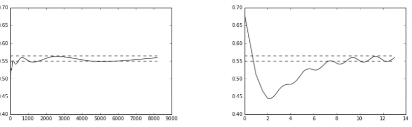
[image:13.595.92.498.308.436.2]i=1πi)n illustrating their oscillatory behaviour.
Figure 4.1. The figure on the left shows the points (n, πn) forn∈ {1,2,3, . . . ,213},
and the figure on the right shows the points (loglog 2n, πn) forn∈ {1,2,3, . . . ,213}; the
numbers πn are computed using formula (4.10). The two horizontal dashed lines intersect the vertical axis at lim infnπn = 23a+31b ≈ 0.51465 and lim supnπn =
1 3a+
2
3b≈0.59863, respectively.
Figure 4.2. The figure on the left shows the points (n,1
n
Pn
i=1πi) for n ∈ {1,
2,3, . . . ,213}, and the figure on the right shows the points (logn
log 2, 1
n
Pn
i=1πi) for n∈ {1,2,3, . . . ,213}; the numbersπ
nare computed using formula (4.10). The two
horizontal dashed lines intersect the vertical axis at lim infnn1Pni=1πi=2 2 3
3 a+ (1− 223
3 )b≈0.54930 and lim supnn1
Pn
i=1πi= (1−2 2 3
3 )a+ 223
[image:13.595.93.500.526.652.2]We will now prove Theorem 4.1.
Proof of Theorem 4.1.
To prove Theorem 4.1, it clearly suffices to show that the box dimensions dimB(X), dimB(X), dimHB,1(X) and dimHB,1(X) are given by the formulas in the statement of Theorem 4.1. Indeed, If we can show that the box dimensions dimB(X), dimB(X), dimHB,1(X) and dim
H
B,1(X) are given by
the formulas in the statement of Theorem 4.1, then the remaining statements in Theorem 4.1 follow immediately from Theorem 2.1. The formulas for the lower and upper box dimensions of X follow from routine arguments and the proofs are therefore omitted. We will now prove the formulas for the 1’st order average box dimensions ofX, i.e. we will prove that
dimHB,1(X) =223 3 a+
1−223 3
b ,
dimHB,1(X) =
1−223 3
a+2
2 3 3 b .
Recall, that it follows from (4.6) that
dimHB,1(X) = lim inf K 1 K K X k=1 πk,
dimHB,1(X) = lim sup K 1 K K X k=1
πk.
(4.7)
Below we will compute the numbers lim infKK1
PK
k=1πk and lim supK
1
K
PK
k=1πk. We start by introducing the following notation. Let
Mn =
X
k≤n
Nk = 2n−1, Mno=
X
k≤n kis odd
Nk, Mne =
X
k≤n kis even
Nk,
We first note that straight forward calculations show that there are bounded sequences (ρen)n and (ρo
n)n such that Mne =
1 32
n+ρe
n ifnis even;
1 62
n+ρo
n ifnis odd,
Mno=
1 62
n+ρe
n ifnis even;
1 32
n+ρo
n ifnis odd.
(4.8)
Similarly, straight forward calculations show that there are sequences (σne)n and (σno)n with σen 2n →0
and σon
2n →0 such that X
i<n iis even
Mne =
1 92
n+σe
n ifnis even;
2 92
n+σo
n ifnis odd,
X
i<n iis odd
Mno=
2 92
n+σe
n ifnis even;
1 92
n+σo
n ifnis odd.
(4.9)
Next, write
λn=
b ifnis even;
a ifnis odd;
recall, thata= log 2log 5 andb=log 3log 5. Finally, we note that a straightforward calculation shows that:
ifMn ≤k≤Mn+1,then πk =
Mne(a−λn) +Mno(b−λn)
k +λn (4.10)
We can now compute the numbers lim infK K1 P K
k=1πk and lim supK
1
K
PK
k=1πk. We begin by deriving an explicit expression for the sum K1 PK
k=1πk. LetK be a positive integer and letn(K) be
the unique integer such that
We now have 1 K K X k=1
πk =AK+BK (4.11)
where
AK = 1 K
Mn(K)−1 X
k=1
πk, BK= 1 K
K
X
k=Mn(K)
πk.
We will now analyse the sumsAK andBK; this is the contents of Claim 1 and Claim 2, respectively.
Claim 1. There is a sequence(sK)K with sK→0 such that
AK =
(
(13b+2 log 29 (b−a) +32a)2n(K)K−1 +sK ifn(K)is even;
(23b−2 log 29 (b−a) +31a)2n(K)K−1 +sK ifn(K)is odd. Proof of Claim 1. Writeui =P
Mi+1−1
k=Mi 1
k and note thatui =
RMi+1
Mi 1
xdx+εi = log( Mi+1
Mi ) +εi =
log 2 +εi where εi→0. Hence, using (4.10), we have
AK= 1 K
X
i<n(K)
(Mie(a−λi) +Mio(b−λi))ui+ 1 K
X
i<n(K)
λiNi+1
= 1 K
X
i<n(K)
iis odd
(Mie(a−λi) +Mio(b−λi))ui+a 1 K
X
i<n(K)
iis odd
Ni+1
+ 1 K
X
i<n(K)
iis even
(Mie(a−λi) +Mio(b−λi))ui+b1 K
X
i<n(K)
iis even
Ni+1
=b 1 KM
o
n(K)+ (b−a)
1 K X
i<n(K)
iis odd
Mioui− X
i<n(K)
iis even
Mieui
+a1 KM
e n(K)
=b 1 KM
o
n(K)+ (b−a)
1 K X
i<n(K)
iis odd
Mio(log 2 +εi)− X
i<n(K)
iis even
Mie(log 2 +εi)
+a1 KM
e n(K)
=b 1 KM
o
n(K)+ (b−a)(log 2)
1 K X
i<n(K)
iis odd
Mio−
X
i<n(K)
iis even
Mie
+a1 KM
e
n(K)+σK, (4.12)
whereσK = (b−a)K1(
P
i<n(K)
iis odd
Mo
iεi−Pi<n(K)
iis even
Me
iεi). Since it follows from (4.9) that supK
1
K
P
i<n(K)
iis odd
Mo i <
∞and supK K1
P
i<n(K)
iis even
Mie<∞, we now conclude that
σK →0. (4.13)
Finally, the desired result follows from a lengthy but straight forward calculation using (4.8), (4.9), (4.12) and (4.13). This completes the proof of Claim 1.
Claim 2. There is a sequence(tK)K withtK →0 such that
BK =
( 2
3(b−a) 2n(K)−1
K log
2n(K)−1
K +b−b
2n(K)−1
K +tK ifn(K)is even;
−2 3(b−a)
2n(K)−1
K log
2n(K)−1
K +a−a
2n(K)−1
Proof of Claim 2. Put vK =P K k=Mn(K)
1
k and note that vK =
RK
Mn(K) 1
xdx+δK = log( K
Mn(K)) +δK
whereδK →0. A simple calculation using (4.8) shows that
BK = 1 K(M
e
n(K)(a−λn(K)) +Mno(K)(b−λn(K)))vK+λn(K)
1
K(K−Mn(K)) = (Mne(K)(a−λn(K)) +Mno(K)(b−λn(K)))
1 K
log
K
Mn(K)
+δK
+λn(K)
1− 1
KMn(K)
= (Mne(K)(a−λn(K)) +Mno(K)(b−λn(K)))
1 Klog
K
Mn(K)
+λn(K)
1− 1
KMn(K)
+τK (4.14) whereτK = (Mne(K)(a−λn(K))+Mno(K)(b−λn(K)))K1δK. Since it follows from (4.8) that supK K1M
e n(K)<
∞and supK K1Mo
n(K)<∞, we now conclude that
τK →0. (4.15)
Finally, the desired result follows from a lengthy but straight forward calculation using (4.8), (4.14) and (4.15). This completes the proof of Claim 2.
We will now combine the expressions for AK and BK in Claim 1 and Claim 2, respectively, to derive an explicit expression for K1 PK
k=1πk=AK+BK. Definef : (0,∞)→Rby
f(x) =−2(3−9log 2)(b−a)x+23(b−a)xlogx . Combining Claim 1 and Claim 2 now shows that
1 K
K
X
k=1
πk =AK+BK=
(
f(2n(K)−1
K ) +b+sK+tK ifn(K) is even;
−f(2n(K)−1
K ) +a+sK+tK ifn(K) is odd.
(4.16)
It follows easily from (4.16) that
lim inf K 1 K K X k=1
πk= min inf
1 2≤x≤1
f(x) +b ,− sup
1 2≤x≤1
f(x) +a
! , lim sup K 1 K K X k=1
πk= max sup
1 2≤x≤1
f(x) +b ,− inf
1 2≤x≤1
f(x) +a
!
.
(4.17)
Finally, a routine calculus argument shows that
min inf
1 2≤x≤1
f(x) +b ,− sup
1 2≤x≤1
f(x) +a
!
= 2
2 3 3 a+
1−223 3
b ,
max sup
1 2≤x≤1
f(x) +b ,− inf
1 2≤x≤1
f(x) +a
!
=
1−223 3
a+2
2 3 3 b .
(4.18)
5. Proof of Theorem 1.1: Preliminary results.
In this section we prove five technical auxiliary lemmas that will be used extensively in Sections 6–8. Recall, that ifE is a subset ofRm andδ >0, then Nδ(E) is the number ofδ-mesh cubes that
intersectE, see (1.2) and (1.3). Also, E denotes the closure ofE in Rm. Lemma 5.1. Fix a bounded subset E of Rm. Letc >1.
(1) For all δ >0, we have Nδ(E)≤(c+ 2)mNcδ(E). (2) For all δ >0, we have Ncδ(E)≤2mNδ(E).
Proof.
This follows from standard arguments, and for the sake of brevity we have therefore decided to omit
the proof.
Lemma 5.2. Let Π = (Πt)t≥t0 be an averaging system. Fix a bounded subset E of R
m. Then we
have
dimΠ,B(E) = dimΠ,B(E), dimΠ,B(E) = dimΠ,B(E).
Proof.
It is easily seen thatNδ(E)≤Nδ(E)≤3mNδ(E) for all δ >0, whence
Z logN
e−s(E)
s dΠt(s)≤
Z logN
e−s(E)
s dΠt(s)≤k
Z
f dΠt+
Z logN
e−s(E)
s dΠt(s), (5.1) wherek= log(3m) and where the functionf : (0,∞)→[0,∞) is defined byf(t) = 1
t. Sincef(t)→0 as t → ∞, we conclude from the Consistency Condition (i.e. Condition (iii)) in the definition of an average system thatR
f dΠt→0 ast→ ∞, and the desired result now follows from this and (5.1). Lemma 5.3. Fix a bounded subsetX of Rd. Letf ∈Cu(X)and r >0. Then there is a polynomial
p:Rd→Rsuch that kf−p|Xk∞< r. Proof.
Since f is uniformly continuous onX, it follows from [Si, p. 78] that there is a continuous function F : X → R such that F|X = f. Next, since X is compact, we conclude from Stone-Weierstrass’ Theorem that there is is a polynomialp:Rd→Rsuch thatkF−p|Xk∞< r, see, for example, [Ca, p. 198, Exercise 24]. In particular, we now conclude thatkf−p|Xk∞=kF|X−p|Xk∞≤ kF−p|Xk∞< r.
Lemma 5.4. Fix a bounded subsetX ofRd. Letf ∈C
u(X)and let p:Rd→Rbe a polynomial. Let
λ∈Rwith λ6= 0. Then there are constantsc >1 andC >1 such that for all δ >0, we have
1
CNcδ graph(p|X+λf)
≤Nδ graph(f)
≤C Nδ
c graph(p|X+λf)
.
Proof.
DefineF : graph(f)→graph(p|X+λf) byF(x, f(x)) = (x, p(x) +λf(x)) and note thatF is bijective withF−1(x, p(x) +λf(x)) = (x, f(x)). An easy calculation shows that bothF andF−1are Lipschitz
maps, and it is not difficult to see that this implies that are constantsc, C >1 such that for allδ >0, we have
1
CNcδ F(graph(f))
≤Nδ graph(f)
≤C Nδ
c F(graph(f))
.
Since clearlyF(graph(f)) = graph(p|X+λf), the desired conclusion follows from the above
Lemma 5.5. LetΠ = (Πt)t≥t0 be an averaging system. Fix a bounded subsetX ofR
d. Letf ∈Cu(X)
and letp:Rd→
Rbe a polynomial. Let λ∈Rwithλ6= 0.
(1) We have
dimΠ,Bgraph p|X+λf
= dimΠ,B graph f, dimΠ,B
graph p|X+λf
= dimΠ,B graph f
.
(2) We have
dimΠ,B graph p|X
= dimΠ,B(X), dimΠ,B graph p|X
= dimΠ,B(X).
Proof.
(1) It follows from Lemma 5.4 that there are constantsc >1 andC >1 such that 1
CNcδ graph(p|X+λf)
≤Nδ graph(f)≤C Nδ
c graph(p|X+λf)
for allδ >0, and Lemma 5.1.(1) therefore implies that 1
C(c+ 2)dNδ graph(p|X+λf)
≤Nδ graph(f)≤C(c+ 2)dNδ graph(p|X+λf)
for allδ >0. We conclude from the above inequality that
−k
Z 1
sdΠt(s)+
Z logN
e−s graph(p|X+λf)
s dΠt(s)
≤
Z logN
e−s graph(f)
s dΠt(s)
≤k
Z 1
sdΠt(s) +
Z logN
e−s graph(p|X+λf)
s dΠt(s), (5.2)
wherek= log(C(c+2)d). Finally, since1
t →0 ast→ ∞, we conclude from the Consistency Condition (i.e. Condition (iii)) in the definition of an average system that R 1sdΠt(s)→0 as t → ∞, and the desired result now follows immediately from this and (5.2).
(2) This statement follows from Part (1) by puttingf = 0 andλ= 1. Lemma 5.6. Let Π = (Πt)t≥t0 be an averaging system. Fix a bounded subsetX of R
d. Let (r n)n be
a strictly decreasing sequence of positive real numbers withrn→0 and logrn
logrn+1 →1. Fort >0, let nt
be the unique positive integer such that
rnt+1≤e−t< rnt.
Then
dimΠ,B(E) = lim inf t
Z logNr ns(E)
−logrns dΠt(s), dimΠ,B(E) = lim sup
t
Z logNr ns(E)
−logrns
dΠt(s).
Proof.
We first note that it follows from Lemma 5.1 that Ne−t(E)≤
rnt e−t + 2
d
Nrnt(E)≤
3 rnt
rnt+1 d
Nrnt(E), Nrnt(E)≤2dNrnt+1(E)≤2dre−t
nt+1 + 2 d
Ne−t(E)≤
6 rnt
rnt+1 d
for allt >0. It follows from this that logNe−t(E)
t ≤
log((3 rnt
rnt+1)
dNr
nt(E))
−logrnt
=f(t) +logNrnt(E)
−logrnt
,
logNrnt(E)
−logrnt ≤
log((6 rnt
rnt+1)
dN e−t(E))
−logrnt =g(t) +
logNe−t(E)
−logrnt
≤g(t) +logrnt+1
logrnt
logNe−t(E)
t =g(t) +h(t) +
logNe−t(E)
t ,
for allt >0, and so
−
Z
f dΠt+
Z logN
e−s(E)
s dΠt(s)
≤
Z logN
rns(E)
−logrns dΠt(s)
≤
Z
g dΠt+
Z
h dΠt+
Z logN
e−s(E)
s dΠt(s), (5.3)
where the functions f, g, h : (0,∞) → [0,∞) are defined by f(t) = −d(loglog 3r
nt + 1−
logrnt+1 logrnt ), g(t) = −d(loglog 6r
nt + 1−
logrnt+1
logrnt ) and h(t) = (
logrnt+1 logrnt −1)
logNe−t(E)
t . Since
logrn+1
logrn → 1 and
lim suptlogNe−t(E)
t = dimB(E)≤d, we conclude thatf(t)→0,g(t)→0 andh(t)→0, whence
Z
f dΠt→0,
Z
g dΠt→0,
Z
h dΠt→0. (5.4)
The desired conclusion follows from combining (5.3) and (5.4).
6. Proof of Theorem 1.1.(2).
The purpose of this section is to prove Theorem 1.1.(2). We first prove three auxiliary lemmas. The first lemma (i.e. Lemma 6.1) is standard and is a suitable version of the reverse Fatou’s lemma. Lemma 6.1. The reverse Fatou’s Lemma [St, Theorem 3.2.3]. Let (M,E, µ) be a measure space and let(ϕn)n be a sequence of positive measurable functionsϕn:M →[0,∞]. IfR supnϕndµ <
∞, thenlim supn
R
ϕndµ≤R
lim supnϕndµ.
Lemma 6.2. Fix a bounded subset X of Rd. Letf ∈Cu(X)andδ >0. Then there is a positive real
numberr >0 such that ifg∈B(f, r), then
Nδ graph(g)≤Nδ graph(f).
Proof.
Let
r=1
2 Q0∈Qinfd+1 δ
Q0∩graph(f)6=∅
inf Q00∈Qd+1
δ
Q00∩graph(f) =∅
dist(Q0∩ graph(f), Q00)
(recall, that forδ >0, the familyQd+1
δ of δ-cubes inR
d+1 is defined in (1.2)). First note that since
graph(f) is compact, we haver >0. Next, we prove that if g∈B(f, r), then Nδ graph(g)
≤Nδ graph(f)
. (6.2)
Indeed, let Letg∈B(f, r). Sincekf−gk∞< r, it follows from the definition ofrthat n
Q∈ Qd+1
δ
Q∩graph(g)6=∅ o
⊆nQ∈ Qd+1
δ
Q∩ graph(f)6=∅ o
,
Lemma 6.3. Let Π = (Πt)t≥t0 be an averaging system. Fix a bounded subset X of R
d. Let c ∈
R andt≥t0. Then the set
(
f ∈Cu(X)
Z logN
e−s graph(f)
s dΠt(s)< c
)
is open in Cu(X).
Proof.
Write
F =Cu(X)\
(
f ∈Cu(X)
Z logN
e−s graph(f)
s dΠt(s)< c
)
=
(
f ∈Cu(X)
Z logN
e−s graph(f)
s dΠt(s)≥c
)
.
We must now prove that F is closed. We therefore fix a sequence (fn)n in F and f ∈ Cu(X) with
kfn−fk∞→0. We must now prove thatf ∈F, i.e. we must prove that Z logN
e−s graph(f)
s dΠt(s)≥c . (6.3)
For brevity define functions ϕ, ϕn : [t0,∞) → [0,∞) by ϕ(s) =
logNe−s graph(f)
s and ϕn(s) =
logNe−s graph(fn)
s . We now prove the following three claims.
Claim 1. We haveR
supnϕndΠt<∞.
Proof of Claim 1. The measure Πthas compact support, and we can therefore choose T0≥t0, such
that supp Πt⊆[t0, T0]. Also, the setX is bounded, and we can therefore find a real numbera with
X ⊆[−a, a]d. Next, note that sincef is bounded andkf
n−fk∞→0, there is a constantM >0 such
that|fn| ≤M for alln. From the above we now deduce that graph(fn)⊆[−a, a]d×[−M, M] for all n, whenceNe−s(graph(fn))≤Ne−s([−a, a]d×[−M, M])≤(2a+ 2)d(2M + 2)e(d+1)s for allnand all
s, and so
ϕn(s) = logNe−s graph(fn)
s ≤
log((2a+ 2)d(2M+ 2)e(d+1)s)
s ≤
log((2a+ 2)d(2M+ 2)e(d+1)T0)
t0
for all n and all s ∈ [t0, T0]. In particular, since supp Πt ⊆ [t0, T0], we therefore conclude that R
supnϕndΠt = RT0
t0 supnϕndΠt ≤
log((2a+2)d(2M+2)e(d+1)T0)
t0 Πt([t0, T0]) < ∞ This completes the
proof of Claim 1.
Claim 2. We havec≤R
lim supnϕndΠt.
Proof of Claim 2. Sincefn ∈F, we conclude that c≤R logNe−s(graph(fn))
s dΠt(s) =
R
ϕndΠt for all n, whence
c≤lim sup n
Z
ϕndΠt. (6.4)
We also note that it follows from Claim 1 and Lemma 6.1 (i.e. the reverse Fatou’s Lemma) that
lim sup n
Z
ϕndΠt≤
Z
lim sup n
ϕndΠt. (6.5)
The desired result now follows from (6.4) and (6.5). This completes the proof of Claim 2.
Proof of Claim 3. Fixs≥t0. We first note that it follows from Lemma 6.2 that there is a positive
number rs>0 such that ifg ∈B(f, rs), thenNe−s(graph(g))≤Ne−s(graph(f)). Also, since kfn−
fk∞ → 0, there is a positive integer ns such that fn ∈ B(f, rs) for all n ≥ ns. In particular, we conclude thatNe−s(graph(fn))≤Ne−s(graph(f)) for all n≥ns, and so
ϕn(s) =
logNe−s graph(fn)
s ≤
logNe−s graph(f)
s =ϕ(s) for alln≥ns, This clearly implies that lim supnϕn(s)≤ϕ(s). This completes the proof of Claim 3.
Finally, we deduce from Claim 2 and Claim 3 that
c≤
Z
lim sup n
ϕndΠt≤
Z
ϕ dΠt=
Z logN
e−s graph(f)
s dΠt(s).
This proves (6.3).
We now turn towards the proof of Theorem 1.1.(2).
Proof of Theorem 1.1.(2).
We must prove that for a typicalf ∈Cu(X), we have dimΠ,B(graph(f)) = dimΠ,B(X). Because of Part (1) in Theorem 1 it clearly suffices to prove that for a typicalf ∈Cu(X), we have dimΠ,B(graph(f))≤
dimΠ,B(X), i.e. it suffices to prove that the set
M =nf ∈Cu(X)
dimΠ,B(graph(f))>dimΠ,B(X) o
is meagre.
Foru >0, write
Mu=
n
f ∈Cu(X)
dimΠ,B(graph(f))>dimΠ,B(X) +u o
.
Since
M = [ u∈Q
u>0
Mu,
it suffices to show that Mu is meagre for allu∈Qwith u >0. We therefore fix u∈Q withu >0.
Since Cu(X) is a complete metric space when equipped with the uniform norm, it suffices to show that there is a countable family (Gn)nof open and dense subsets ofCu(X) with∩nGn ⊆Cu(X)\Mu.
Fort≥t0, let
Lt=
(
f ∈Cu(X)
Z logN
e−s graph(f)
s dΠt(s)<dimΠ,B(X) +u
)
,
and for a positive integern, put
Gn =
[
t≥n Lt.
Below we show that the family (Gn)n consists of open and dense subsets of Cu(X) with ∩nGn ⊆
Cu(X)\Mu; this is the contents of the following three claims.
Claim 1. The setGn is open in Cu(X).
Proof of Claim 1. Indeed, since it follows from Lemma 6.3 thatLtis open for allt≥t0, we immediately
conclude thatGn=∪t≥nLtis open. This completes the proof of Claim 1
Proof of Claim 2. Letf ∈Cu(X) and letr >0. We must now findg∈Cu(X) such thatkg−fk∞< r
andg∈Gn. We first note that it follows from Lemma 5.3 that there is a polynomialp:Rd →Rsuch
thatkf−p|Xk∞< r. Putg=p|X. It is clear that gis uniformly continuous and thatkg−fk∞< r.
We will now prove thatg∈Gn. It follows from Lemma 5.2 and Lemma 5.5 that
lim inf t→∞
Z logN
e−s graph(g)
s dΠt(s) = dimΠ,B graph(g)
= dimΠ,B graph(g)
= dimΠ,B graph(p|X)
= dimΠ,B(X) <dimΠ,B(X) +u .
This inequality shows that we can findt≥nsuch thatR logNe−s( graph(g) )
s dΠt(s)<dimΠ,B(X) +u, whenceg∈Lt⊆Gn. This completes the proof of Claim 2.
Claim 3. We have∩nGn⊆Cu(X)\Mu.
Proof of Claim 3. Let f ∈ ∩nGn. Hence for each positive integer n, we can find tn ≥ n such that f ∈ Ltn, whence
R logNe−s( graph(f) )
s dΠtn(s) < dimΠ,B(X) +u for all positive integers n, and so lim inft→∞R
logNe−s( graph(f) )
s dΠt(s) ≤ lim infn
R logNe−s( graph(f) )
s dΠtn(s) ≤ dimΠ,B(X) +u. It follows from this thatf ∈Cu(X)\Mu. This completes the proof of Claim 3.
Combining Claim 1, Claim 2 and Claim 3, we now conclude thatMu is meagre.
7. Proof of Theorem 1.1.(3).(i)
The purpose of this section is to prove Theorem 1.1.(3).(i). We start by providing an alternative characterization of the box dimension (see Lemma 7.1) based on open cubes (as opposed to the usual definition (1.2)-(1.5) based on closed cubes). The motivation for introducing this characterization is the following. Namely, the proof of Theorem 1.1.(3).(i) requires a lower bound for the upper box dimension of the graph of a typical function, and methods for establishing good lower bounds for the box dimension of subsetsE ofRmare often sensitive to the number of cubes from the grid Qmδ who only intersectE by their boundaries. It is to overcome this problem that we provide an alternative characterization of the box dimension based on open cubes. We first introduce some notation. For δ >0 andu∈Rm write
Q◦u,m,δ =
( m
Y
i=1
(niδ,(ni+ 1)δ)
(n1, . . . , nm)∈u+Zm
)
. (7.1)
Also, for a subset E of Rm, we will write N◦
u,δ(E) for the number of open boxes from Q
◦,m
u,δ that intersectE, i.e.
Nu◦,δ(E) =
n
Q∈ Q◦u,m,δ
Q∩E6=∅ o
.
Finally, we write
Um=
n
(u1, . . . , um)
ui= 0,
1 2 o
.
and put
Nδ◦(E) =
X
u∈Um
Lemma 7.1. Fix a bounded subset E of Rm.
(1) For all δ >0, we have Nδ◦(E)≤3mNδ(E).
(2) For all δ >0, we have Nδ(E)≤3mNδ◦(E).
(3) Let Π = (Πt)t≥t0 be an averaging system. We have
dimΠ,B(E) = lim inf t
Z logN◦
e−s(E)
s dΠt(s),
dimΠ,B(E) = lim sup
t
Z logN◦
e−s(E)
s dΠt(s).
Proof.
(1)-(2) This follows from standard arguments, and for the sake of brevity we have therefore decided to omit the proof.
(3) It follows from (1) and (2) that
−k
Z
f dΠt+
Z logN
e−s(E)
s dΠt(s)≤
Z logN◦
e−s(E)
s dΠt(s)≤k
Z
f dΠt+
Z logN
e−s(E)
s dΠt(s), (7.3) wherek= log(3m) and where the functionf : (0,∞)→[0,∞) is defined byf(t) = 1t. Sincef(t)→0 as t→ ∞, we deduce thatR
f dΠt→0 as t→ ∞, and the desired result now follows from this and
(7.3).
Lemma 7.2. Fix a bounded subset X of Rd. Letf ∈C
u(X)andδ >0. Then there is a positive real
numberr >0 such that ifg∈B(f, r), then
Nδ◦(graph(f))≤Nδ◦(graph(g)).
Proof.
For eachu= (u1, . . . , ud+1)∈Ud+1, write
Eu,δ=
[
m∈ud+1+Z
Rd× {mδ}
,
i.e. theEu,δ’s denote the “horizontal” hyperplanes that outline the gridQ◦ ,d+1
u,δ . For eachQ∈ Q
◦,d+1 u,δ withQ∩graph(f)6=∅, choosexQ∈Q∩graph(f) and put
r=1 2u∈minUd+1
min Q∈Q◦,d+1
u,δ
Q∩graph(f)6=∅
dist(xQ, Eu,δ).
We first prove thatr >0. Indeed, for allu∈Ud+1 andQ∈ Q◦
,d+1
u,δ withQ∩graph(f)6=∅we have xQ ∈Q∩graph(f)⊆Q, whencexQ 6∈Eu,δ. We conclude from this that dist(xQ, Eu,δ)>0, and so
r >0. Next we prove that ifg∈B(f, r), then
Nδ◦(graph(f))≤Nδ◦(graph(g)). (7.4) Indeed, letg∈B(f, r). Sincekf−gk∞< r, the definition ofr implies that ifu∈Ud+1, then
n
Q∈ Q◦u,d,δ+1
Q∩graph(f)6=∅ o
⊆nQ∈ Q◦u,d,δ+1
Q∩graph(g)6=∅ o
.
Lemma 7.3. Let Π = (Πt)t≥t0 be an averaging system. Fix a bounded subset X of R
d. Let c ∈
R andt≥t0. Then the set
(
f ∈Cu(X)
Z logN◦
e−s(graph(f))
s dΠt(s)> c
)
is open in Cu(X). Proof.
Write
F =Cu(X)\
(
f ∈Cu(X)
Z logN◦
e−s(graph(f))
s dΠt(s)> c
)
=
(
f ∈Cu(X)
Z logN◦
e−s(graph(f))
s dΠt(s)≤c
)
.
We must now prove that F is closed. We therefore fix a sequence (fn)n in F and f ∈ Cu(X) with
kfn−fk∞→0. We must now prove thatf ∈F, i.e. we must prove that Z logN◦
e−s(graph(f))
s dΠt(s)≤c . (7.5)
For brevity define functions ϕ, ϕn : [t0,∞) → [0,∞) by ϕ(s) = logN◦
e−s(graph(f))
s and ϕn(s) =
logN◦
e−s(graph(fn))
s . We now prove the following two claims.
Claim 1. We haveR
lim infnϕndΠt≤c.
Proof of Claim 1. Sincefn ∈F, we conclude that R
ϕndΠt =R logNe◦−s(graph(fn))
s dΠt(s)≤c for all n, whence
lim inf n
Z
ϕndΠt≤c . (7.6)
We also note that it follows from Fatou’s lemma that
Z
lim inf
n ϕndΠt≤lim infn
Z
ϕndΠt. (7.7)
The desired result now follows from (7.6) and (7.7). This competes the proof of Claim 2.
Claim 2. For all s≥t0, we haveϕ(s)≤lim infnϕn(s).
Proof of Claim 2. Fixs≥t0. We first note that it follows from Lemma 7.2 that there is a positive
number rs>0 such that ifg ∈B(f, rs), thenNe◦−s(graph(f))≤Ne◦−s(graph(g)). Also, since kfn−
fk∞ → 0, there is a positive integer ns such that fn ∈ B(f, rs) for all n ≥ ns. In particular, we
conclude thatNe◦−s(graph(f))≤Ne◦−s(graph(fn)) for all n≥ns, and so
ϕ(s) = logN
◦
e−s(graph(f))
s ≤
logNe◦−s(graph(fn))
s =ϕn(s) for all n≥ns, This clearly implies thatϕ(s)≤lim infnϕn(s). This completes the proof of Claim 2.
Finally, we deduce from Claim 1 and Claim 2 that
Z logN◦
e−s(graph(f))
s dΠt(s) =
Z
ϕ dΠt≤
Z
lim inf
n ϕndΠt≤c .
This proves (7.5).
Proof of Theorem 1.1.(3).(i).
For brevity write A = supf∈Cu(X)dimΠ,B(graph(f)). We must prove that for a typical f ∈ Cu(X),
we have dimΠ,B(graph(f)) = A. It clearly suffices to prove that for a typical f ∈ Cu(X), we have
dimΠ,B(graph(f))≥A, i.e. it suffices to prove that the set
M =nf ∈Cu(X)
dimΠ,B(graph(f))< A o
is meagre.
Foru >0, write
Mu=nf ∈Cu(X)
dimΠ,B(graph(f))< A−u o
.
Since
M = [ u∈Q
u>0
Mu,
it clearly suffices to show that Mu is meagre for all u ∈ Q with u > 0. We therefore fix u ∈ Q
with u > 0. Since Cu(X) is a complete metric space when equipped with the uniform norm, it suffices to show that there is a countable family (Gn)n of open and dense subsets of Cu(X) with
∩nGn⊆Cu(X)\Mu. Fort≥t0, let
Lt=
(
f ∈Cu(X)
Z logN◦
e−s(graph(f))
s dΠt(s)> A−u
)
,
and for a positive integern, put
Gn =
[
t≥n Lt.
Below we show that the family (Gn)n consists of open and dense subsets of Cu(X) with ∩nGn ⊆
Cu(X)\Mu; this is the contents of the following three claims.
Claim 1. The setGn is open in Cu(X).
Proof of Claim 1. Indeed, since it follows from Lemma 7.3 thatLtis open for allt≥t0, we immediately
conclude thatGn=∪t≥nLtis open. This completes the proof of Claim 1
Claim 2. The setLn is dense in Cu(X).
Proof of Claim 2. Letf ∈Cu(X) and letr >0. We must now findg∈Gn such thatkg−fk∞< r.
Without loss of generality, we may assume r2 ≤u. We first note that it follows from Lemma 5.3 that there is a polynomialp:Rd→
Rsuch thatkf −p|Xk∞< r. We also note that the definition of
Aimplies that there is a function ϕ∈Cu(X) such that dimΠ,B(graph(ϕ))> A−
r
4. (7.8)
Finally, put c = r
4(kϕk∞+1) > 0, and define g : X → R by g =p|X+cϕ. Clearly g ∈ Cu(X) and
kf −gk∞ =kf −p|X−cϕk∞ ≤ kf −p|Xk∞+ckϕk∞ =kF|X−p|Xk∞+ckϕk∞ ≤ r4 +ckϕk∞ ≤
r
4 +
r
4(kϕk∞+1)kϕk∞ < r. Next, we show that g ∈ Gn. We first note that it follows from Lemma
7.1 that lim supt→∞R logN ◦
e−s(graph(f))
s dΠt(s) = dimΠ,B(graph(g)), and we can therefore chooset≥n such that
Z logN◦
e−s(graph(g))
s dΠt(s)>dimΠ,B(graph(g))− r
4. (7.9)
Since r2 ≤u, we conclude from (7.9) that
Z logN◦
e−s(graph(g))
s dΠt(s) +u≥
Z logN◦
e−s(graph(g))
s dΠt(s) +
r 2
≥dimΠ,B(graph(g)) + r 4 = dimΠ,B(graph(p|X+cϕ)) +
r
Also, observe that it follows from Lemma 5.5 that dimΠ,B(graph(p|X+cϕ)) = dimΠ,B(graph(ϕ)), and
we therefore conclude from (7.10) that
Z logN◦
e−s(graph(g))
s dΠt(s) +u≥dimΠ,B(graph(ϕ)) + r
4. (7.11)
Finally, combining (7.8) and (7.11) yields
Z logN◦
e−s(graph(g))
s dΠt(s) +u > A
This shows thatg∈Lt⊆Gn. This completes the proof of Claim 2.
Claim 3. We have∩nGn⊆Cu(X)\Mu.
Proof of Claim 3. Letf ∈ ∩nGn. Hence for each positive integern, we can find a real numbertn≥n such that f ∈ Ltn, whence
R logNe◦−s( graph(f) )
s dΠtn(s) > A−u for all positive integers n, and so
lim supt→∞R logN
◦
e−s( graph(f) )
s dΠt(s)≥lim supn
R logNe◦−s( graph(f) )
s dΠtn(s)≥A−u. It follows from
this thatf ∈Cu(X)\Mu. This completes the proof of Claim 3.
Combining Claim 1, Claim 2 and Claim 3, we now conclude thatMu is meagre.
8. Proof of Theorem 1.1.(3).(ii).
The purpose of this section is to prove Theorem 1.1.(3).(ii).
Proposition 8.1. LetX be a bounded subset ofRd with only finitely many isolated points. Letε >0
Then there is a functionf ∈Cu(X) such that
N2−n(graph(f))≥2−dN2−n(X) 2n(1−ε)
for all positive integers n.
Proof.
Observe that if a set has finitely many isolated points, we may remove these without changing the lower and the upper box dimensions of the set. Hence we may suppose thatX has no isolated points.
Fix a positive integernand write
Vn=
n
Q∈ Qd
2−n
Q∩X 6=∅ o
(recall, that for δ > 0, the family Qd
δ of δ-cubes inR
d is defined in (1.2)). Since X does not have isolated points there is a subfamilyWn ofVn with|Wn| ≥ 21d|Vn|such that ifQ∈ Wn, then none of
the points in the setX∩Qare isolated inX∩Q.
For each integernwithn≥0, we will now define a uniformly continuous functionfn :X →[0,∞) and a finite set
En=nxQ,n
Q∈ Wn o
∪ nyQ,n,i
Q∈ Wn, i= 1, . . . ,
2n(1−ε)o such that the following properties are satisfied
xQ,n, yQ,n,i∈X∩Q , (8.1)
n−1 X
j=0
fj(xQ,n)− n−1 X
j=0
fj(yQ,n,i)
kfnk∞≤52n(1−ε)2−n, (8.3)
fn(xQ,n) = 0, (8.4)
fn(yQ,n,i) = 5i2−n, (8.5)
fk(yQ,n,i) = 0 fork < n . (8.6) Below we construct the functionsfn and the setsEn inductively as follows.
First we put f0 = 0 and E0 = ∅. Next assume that the functions f0, f1, . . . , fn−1 and the
sets E0, E1, . . . , En−1 have been constructed such that properties (8.1)–(8.6) are satisfied. We will
now construct fn and En. Fix Q ∈ Wn. It follows from the definition of Wn that we can choose xQ,n∈(Q∩X)\(E0∪E1∪. . .∪En−1). It also follows from the definition of Wn and the fact that the functionsf0, f1, . . . , fn−1 are (uniformly) continuous that we can choose pointsyQ,n,i∈(Q∩X)\ (E0∪E1∪. . .∪En−1) with i = 1, . . . ,
2n(1−ε)
such that the pointsxQ,n, yQ,n,1, . . . , yQ,n,d2n(1−ε)e
are distinct and
n−1 X
j=0
fj(xQ,n)−
n−1 X j=0 fj(yQ,n,i)
≤2−n Now definegn :E0∪E1∪. . .∪En−1∪En→Rby
gn(x) =
0 ifx∈E0∪E1∪. . .∪En−1;
0 ifx=xQ,n; 5i2−n ifx=y
Q,n,i fori= 1, . . . ,
2n(1−ε)
.
Next, observe that since the setE0∪E1∪. . .∪En−1∪En is finite, we can find a uniformly continuous
functionfn:X→[0,∞) such thatfn|E0∪E1∪...∪En−1∪En =gnand 0 = minx∈E0∪E1∪...∪En−1∪Engn(x)≤
f(x)≤maxx∈E0∪E1∪...∪En−1∪Engn(x) = 5
2n(1−ε)
2−n for allx∈X. It is clear that the functionf n and the set En ={xQ,n|Q∈ Wn} ∪ {yQ,n,i|Q∈ Wn, i = 1, . . . ,
2n(1−ε)
} satisfy the properties in (8.1)–(8.6). This completes the construction of the functionsfn and the setsEn.
We now constructf ∈Cu(K) as follows. Namely, note that it follows from (8.3) that
X
n
kfnk∞≤ X
n
52n(1−ε)2−n
≤5X
n
2−nε+ 2−n
<∞. (8.7)
We conclude from (8.7) that the functionf defined by f =X
n fn
is a well-defined real valued uniformly continuous function. Below we prove that
N2−n(graph(f))≥2−dN2−n(X) 2n(1−ε)
for alln. This is done in the following 2 claims.
Claim 1. Ifnis a positive integer and Q∈ Wn, thenN2−n(graph(f|Q∩X))≥2n(1−ε).
Proof of Claim 1. We first show that ifi, j= 1, . . . ,
2n(1−ε)
withi6=j, then
|f(yQ,n,i)−f(yQ,n,j)|>2−n. (8.8) Indeed, we have
|fn(yQ,n,i)−fn(yQ,n,j)|
= n X k=0 fk(yQ,n,i)− n X k=0 fk(yQ,n,j) ! −
n−1 X
k=0
fk(yQ,n,i)−
n−1 X k=0 fk(yQ,n,j) ! ≤ n X k=0 fk(yQ,n,i)− n X k=0 fk(yQ,n,j) +
n−1 X
k=0
fk(yQ,n,i)−
n−1 X k=0 fk(xQ,n) +
n−1 X
k=0
fk(xQ,n)−