A reference architecture and model for sensor data warehousing

A Reference Architecture and Model for

Sensor Data Warehousing

Simon Dobson,

Senior Member, IEEE,

Matteo Golfarelli, Simone Graziani, and Stefano Rizzi

Abstract—Sensor data is becoming far more available thanks to the growth in both sensor systems and Internet of Things devices. Much of the value of sensor data comes from examining trends that occur over long timescales, ranging from hours to years. However, making use of data a long time after it has been collected has significant implications for the data-handling systems used to manage it. In particular, the data must be contextualised into the environment in which it was collected to avoid misleading (and potentially dangerous) mis-interpretation. We apply data warehousing techniques to develop an extensible model to capture contextual metadata alongside sensor datasets, and show how this can be used to support the analysis of datasets long after collection. We present our baseline reference framework for sensor context and derive multidimensional schemata representing different modelling and analysis scenarios. Finally, we exercise the model with two case studies.

Index Terms—Data Warehouse, Multidimensional Modelling, Sensor Networks, Data Analytics

F

1

I

T

in the coming years, fueled by growth both in “explicit” sensor systems and in the increased “implicit” capabilities of the Internet of Things (IoT). Sensing provides stakeholders with data upon which to base decisions that have increasing importance in managing a huge range of user-centred and societal problems.

Much of the value of sensor data comes from examining the trends and variations that occur over long timescales — where “long” may range from hours to years, depending on the context of data collection. This is the point at which sensor data becomes “big data” that can be manipulated using machine learning and other tools from data analytics. The goal of such approaches is to extract further global information from the time series, over and above the local information (in space and time) that may be used opera-tionally. That is to say, the value of a sensor dataset may come both from short-term, tactical, operational use of the information it contains, and also from long-term, strategic uses that permit identification of trends and features that

are relevant to future contingency planning and post facto

analysis of operations. In many contexts these multiple uses significantly increase the importance and value of any data collected, making the financial case for instrumenting environments stronger: indeed, many sensor deployments are financially viable only when considered from the per-spective of years-worth of data collection.

There is, however, a big challenge implicit in this sce-nario. Making use of data a long time after it has been col-lected implies a number of things about the data handling

• Simon Dobson is with the School of Computer Science, University of St Andrews, St Andrews, Fife KY16 9SX UK (e-mail: [email protected]).

• Matteo Golfarelli, Simone Graziani, and Stefano Rizzi are with DISI, University of Bologna, V. le Risorgimento 2, 40136 Bologna IT (e-mail: [email protected], [email protected], [email protected]).

system used to manage it. The data must besearchableand

findablein order to be retrieved when required; it must be

parseable in terms of extracting the data types and ranges used for representation; and —most importantly— it must becontextualisedinto the environment in which it was col-lected. By “contextualised” we mean that it must be possible to retrieve the details of the sensors, their installation and operation, as well as simply their data [1].

What particularly makes contextualisation important is the “exposed” lifecycle of a typical sensor. By way of ex-ample, consider an air-quality sensor deployed to measure pollutant gases in an industrial setting. The data acquired from this sensor will typically consist of a stream of num-bers, and clearly we need to retain the units and range of these data points for later analysis. But the sensor’s readings also have metadata such as precision, accuracy, sampling frequency and the like, associated both with the specific transducer being used and the sensing framework controlling it, which must also be recorded if we are to have confidence in analysis. Furthermore the sensor will deteri-orate the longer it is in the field, both through mechanical ageing and (in many cases) chemical and physical changes in the transducer itself, both of which lead to decalibration. It may become occluded by plant life, biofilmed by bacterial action, and dirtied by the actions of the very pollutants it is deployed to measure —all of which will affect its behaviour, and so the values in the time series dataset. Cleaning the

sensor, whether on an ad hoc basis or according to some

schedule, may re-set some of these influences and return the sensor to (some part of) its pristine state.

Similar challenges are well-known in database technol-ogy, where the techniques of data warehousing have been developed to ensure that data held for the long term re-main robustly analysable in the context of Business Intel-ligence (BI) applications. However, these techniques have been applied in the context of sensor networking only to a limited extent, and mostly with a small attention to data modelling issues. In this paper we address this omission by developing data warehousing schemata for sensor data. We develop an extensible model that allows for the capture of contextual metadata alongside sensor datasets, and show how this can be used to support the long-term analysis of historical datasets. While our proposal is aimed at long-term data management with storage and explorative analyses in mind, it is fully compatible with the adoption of other problem-specific analytical solutions. Indeed, the proposed architecture and multidimensional schemata are meant to provide a foundation which other analytical modules can rely upon in order to access integrated and consistent data. We argue that such an approach will increase the value that can be extracted from collected data, as well for supporting some increased level of confidence in the strategies and decisions such datasets are used to support.

The remainder of the paper is organized as follows. Section 2 introduces the basics of data warehousing and multidimensional modelling, and the necessary concepts and technologies in sensor data representation. Section 3 presents our baseline reference framework for sensor con-text, from which Section 4 then derives multidimensional schemata representing different modelling and analysis sce-narios. We exercise the model in Section 5 with two case studies, which we then use in Section 6 to draw some conclusions and future directions.

2

B

The topic of sensor network modelling has been tackled from many different perspectives. The result is a plethora of approaches whose main goals are either to enable interoper-ability between processes, or to simplify the analysis of data and the design of applications. In this section we survey the most relevant of these approaches, after first providing some basic notions of data warehousing and multidimensional modelling.

2.1 Data warehouses and data lakes

Operational databases are a common feature of informa-tion systems, where they enable long-term, language- and application-neutral storage of large volumes of data for running a company’s daily business operations. While a goal of database design is to represent the data in a natural, “normal” form, performance and other constraints often dictate part of the data layout. This often involves compro-mises between meeting different applications’ requirements, as well as in issues such as performing data denormalisation for performance reasons. While such compromises are often necessary for production systems, they harm the ability to access data over the long term. The danger is that data that remains uncurated for a long period may become inaccessible, or so inconsistent as to be useless.

Data warehousing is a process for ensuring the long-term viability of data storage and retrieval using a single

integrated repository called a Data Warehouse (DW) that

is aimed at supporting analysis and decision-making. It starts from the recognition that the schemata appropriate for archival storage may differ from those needed for opera-tional use. Rather than trying to find a compromise between the two, dara warehousing instead develops structured pro-cesses for transforming between them. A generic data ware-housing architecture normally uses some of the company’s operational databases as data sources; while these databases are most often heterogeneous and inconsistent with each

other, a DW represents all this data within asingleschema.

Between the sources and the DW is a process of Extract,

Transform, and Load (ETL)which consolidates the multiform data in the operational databases into the uniform structure of the DW. ETL is a periodic and incremental process that also includes data cleansing steps to resolve inconsistencies and remove noise —which may be tolerated in the opera-tional databases but not in the DW.

Modern enterprise architectures are often extended with a data lake, a repository based on low-cost technologies that contains large quantities of raw, unstructured or semi-structured data [3]. Intuitively, the data lake is the place for storing, in its native form, current data that is being produced by the various operational processes that make up the enterprise; by contrast, the DW represents the cu-rated set of events that occurred, that can be used by

post factotrend analysis, anomaly detection, and other non-operational processes. This separation implies that, as the enterprise changes, the data lake can be freely reconfigured in support of new processes, with corresponding changes to the ETL process to populate the DW. The challenge is then to manage such changes in a stable way within the DW schema.

2.2 Multidimensional modelling and OLAP

The multidimensional model is the foundation for data representation and querying in DW and BI applications [4]. It is based on the observation that the factors affecting

decision-making processes are business-specificfactssuch as

sales, hospital admissions, maintenance, and so on. We refer

to these collections of facts as cubes, although they may in

fact be higher-dimensional. Data is structured as points in

an n-dimensional space, whose coordinates correspond to

categorical dimensions for analysis. Each point represents aneventthat occurred and is described by a set of (usually

numerical)measuresrelevant to decision-making processes.

Normally, each dimension is associated with ahierarchyof

aggregation levelsthat allow events to be grouped in different ways.

In relational implementations of DWs, multidimensional

cubes are normally stored using star schemata [4]. A star

schema is composed by (i) some dimension tables, one for

each hierarchy, each identified by a surrogate key (i.e., a

DBMS-generated progressive identifier) and including one

column for each level of that hierarchy, and (ii) one fact

the number of joins) dimension tables in star schemata are often denormalised (while keeping the rest of the schema normalised).

DW schemata can be designed using any data analysis technique, but specialised techniques also exist that are targeted specifically at multidimensional (as opposed to traditional relational) modelling. In this paper we make use of the Dimensional Fact Model (DFM) [4], which structures the schema in terms of the facts to be analysed, their dimensions, measures, and levels.

The main paradigm for analysing and querying

multi-dimensional cubes isOn-Line Analytical Processing(OLAP).

An OLAP session consists of a sequence of queries, each obtained from the previous one by applying an OLAP operation [4]. Each query groups measured values by some

subset of levels using an aggregation operator (e.g., sum or

average), and optionally applies a selection predicate. The

main OLAP operations are roll-up, which gives a broader

view of a fact by further aggregating data;drill-down, which

gives more detail on a fact by disaggregating data; and

slice-and-dice, which selects either a slice or a dice of the cube by expressing a selection predicate.

2.3 Sensor network data modelling

While DW technologies are part of some proposed sensing architectures, the details on how the data has been modelled are mostly omitted. An example of this can be found in Huo

et alia[5], where the authors present a framework for fault-diagnosis that employs an enterprise DW as an integrated repository for monitoring data, but do not explain the

specific data model adopted. Scrineyet alia [6] proposes a

methodology to obtain multidimensional data cubes start-ing from XML and JSON data sources. The methodology is composed by two main steps: converting an XML or JSON schema definition into a novel graph structure called StarGraph, followed by populating the data cubes with the events coming from the network. The main limitation of this approach is that it works only with XML and JSON data sources that provide a schema definition. Note that the idea of supporting (or even automating) the design of DWs is not new: early approaches date from the 1990s [7], and remains an on-going research effort [8]. However, the issue with these techniques is that they are often tied with specific

types of data sources (e.g., XML/JSON for [6], data vaults for

[8]).

Among the approaches that focus on the interoperability aspect, the SensorML [9] framework provides a set of XML schemata to describe sensor networks from the physical

systems to the measurements and processes involved. Deet

alia[10] present work aimed at improving the

interoperabil-ity aspect of IoT. The result is a semantic model approach where the resources of the network are exposed through web services, enabling semantic search and reasoning over both devices and the data they provide. BOnSAI [11] takes a

more focused approach by specialising other ontologies (e.g.,

OWL-S [12]) for ambient intelligence scenarios: once again, the goal is to create a machine-interpretable representation of sensor networks to improve interoperability.

An interesting tool to support the design of applications over sensor networks is SEM [13], which is a framework

that represents the sensor network through two different metamodels: a functional metamodel and a data metamodel. The former describes the network as a set of exposed ser-vices, while the latter describes the available data sources. Through these two metamodels the application designer can obtain a high-level view of the network to better manage its complexity.

3

R

MODEL

In this section we present our reference framework, which is composed of a functional architecture (section 3.1) and the domain model (section 3.2). This framework will then be used as a reference for all proposed multidimensional schemata and use cases for the rest of the paper.

3.1 Functional architecture of the analytical system

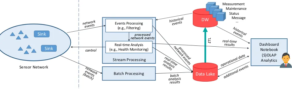
Figure 1 shows the proposed functional architecture that we will use to contextualise the multidimensional schemata presented in section 4 and the use cases presented in sec-tion 5. We start by describing the processes and how they interact, and then proceed to explain how we envision its implementation from a technological perspective.

The architecture shown in figure 1 is separated into two different large-scale areas by the vertical dashed line. On the left there is the sensor network, while on the right there are all the processes that read, elaborate, and store the data coming from that network.

We treat the sensor network as a collection of (typ-ically computationally-constrained) nodes collecting data from the physical environment. The nodes often make use of mesh or other network protocols and use spanning trees for collecting and aggregating data to a small set of “sink” nodes – none of the details of which affect the current work. We simply assume that the data collected is somehow returned to the cloud for processing. (It is

worth noting in passing that many sensor networks are

actually sensor/actuator networks that need to make local

control decisions. Our architecture supports these too, and

would probably want to recordboththe sensed dataandthe

decisions made as a result, for later analysis.)

Users and use cases

The users of the proposed architecture can be grouped into three main agents:

• A data scientist, who has both high IT and analyt-ical skills and can therefore exploit both the well-structured and organised data stored in the DW and the less consistent and structured contents of the data lake to carry out her analyses.

• ABI user, who has broad knowledge about the

do-main of the data but needs accessible analytical BI

tools (e.g., Tableau1_{, MicroStrategy}2_{, and so forth) to}

accomplish her goals. The BI user typically only has access to structured and well-organised data stored in the DW.

Dashboard Notebook (S)OLAP Analytics

Data Lake

ETL

Stream Processing Events Processing

(e.g., Filtering)

Real-time Analysis (e.g., Health Monitoring)

control

Sensor Network Sink

Sink

DW

Measurement Maintenance

Status Message

…

processed network events

Batch Processing

Fig. 1: Functional architecture of the analytical system for sensor networks

• A technician, who is a user who has very specific

domain knowledge but lacks IT skills. These users include, for instance, any maintenance worker who might be interested in monitoring in real-time the status of the network.

The interface capabilities required for different users will change depending on the type of final application. Typically, data scientists and skilled domain users prefer having more

control on data and more powerful tools (e.g., Notebook

tools, OLAP interfaces, and analytics), while domain users prefer simple and focused information such as Key Per-formance Indicators (KPIs) that can be presented through dashboard tools. We will not discuss in details the wide range of possible applications the proposed architecture can be used for: instead, in the following we will discuss in depth the domain model that is needed to support them.

The typical data flow in the architecture sketched in figure 1 can be described as follows. Every event sent by a device in the sensor network to the analytical system is processed in either a streaming or a batch fashion as appro-priate. In the former case the results of the computation can be both directly presented to the end user and also stored in the data lake for future use; in the latter case the results are simply stored in the data lake. When processing events in real time the system might also react and respond to control the network, thus creating a feedback loop. Once the results of the processing have been stored in the data lake, they can be directly accessed by users (data scientists) and ap-plications for further analysis and elaborations. Periodically (which might be hourly, daily, weekly, and so on) the data in the data lake is used to feed the DW through the ETL process. Once in the DW, the events become also available to BI users by means of OLAP analysis tools.

Event processing and storage

Stream processingis one of the two intermediary processes between the sensor on one end and users and storages on the other. The typical output of the sensor network is

considered as a stream of events (e.g., temperature

measure-ments) that must be processed in a timely fashion. In our architecture this process is decomposed into two different

subprocesses, events processing and real-time analysis. The

former includes simple operations such as filtering and

smoothing of the input events, while the latter uses the output of the former and the historical data in the DW to perform more complex (but still stream-based) analyti-cal functions such as forecasting, network monitoring, and so on. We assume that the real-time analysis process can directly interact with the sensor network, for instance for activity regulation purposes.

In certain scenarios it might be either necessary (for ex-ample due to the lack of connectivity) or sufficient (because the timeliness constraints are relaxed) to treat the events coming from the sensor network in larger aggregates rather than singly. In these cases the events produced are handled by batch processing rather than by stream processing. By relaxing timeliness constraints it is possible to perform more complex computations that would not be possible in a real-time scenario. For example, signal reliability techniques can be run at this stage, possibly in conjunction with some more advanced event classification processes [14]. Noisy data can be either tagged or dropped [15] – the latter is often preferable as it allows later analysis of the cleaning processes themselves.

Of course, these styles of processing are not mutually exclusive and, indeed, a mix of the two can be employed to have both real-time results through stream processing and higher quality results from batch processing. The results of both stream and batch processing are loaded into the data lake.

Technology choices

From a technological perspective, this architecture can be implemented as follows. We ignore the implementation of the sensor network other than to assume the creation of a stream of sensed values.

Perhaps the most promising technology for the analytic

system is the Hadoop platform3, which provides distributed

storage and processing capabilities. The choice of a dis-tributed system is almost mandated in many applications, where a traditional centralised approach cannot accommo-date the high data volumes that a sensor network might produce. Furthermore, the Hadoop platform is very flexible and can support many other frameworks that are necessary

for some of the tasks described above. For example, exam-ple frameworks for streaming processing include Apache

Storm4_{, Apache Spark [16], and Apache Flink}5_{. Spark and}

Flink can also take on batch processing tasks.

For storage, the data lake must be able to handle both unstructured and structured data. The simplest and most general solution is accommodating all kinds of unstructured data as simple distributed files in the HDFS filesystem [17] and structured data through either Apache Hive, SparkSQL, or Impala [18]. (An alternative to using HDFS for all un-structured data is that of adopting more specialised storage types, which generally fall into the NoSQL [19] category: we avoid discussing these solutions as they are out of the

scope of this work.) Apache Kylin6 _{provides OLAP}

pro-cessing on top of these (and other) storage and propro-cessing solutions. In particular, it is the first engine in the Hadoop ecosystem natively optimized for OLAP workload: it fully support multidimensional schemata (see section 4), enables incremental refresh of cubes, and provides an interactive experience even when billions of tuples are involved [20].

Finally, there some commercial platforms (e.g., Azure IoT

Suite7_{) that boost the construction of IoT solutions. It is}

worth noting, however, that even in this case, the problem of accurately modelling data has still to be solved.

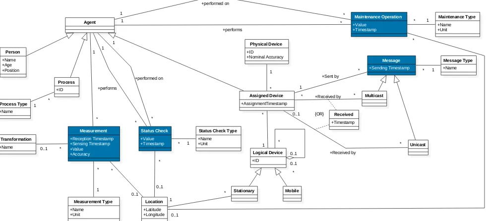
3.2 Domain model

We now briefly describe the main concepts represented in figure 2, which shows the domain model of an analytical system for sensor networks using the notation of a UML class diagram. When feasible, we also use the SensorML framework [9] as a reference and link the described concepts to the corresponding ones in SensorML.

Byagent[21] we mean anything that can be viewed as perceiving its environment and that can act upon it. Agents

interact by way of messages, either unicast or multicast

between them. We distinguish the following types of agent:

Device APhysical Deviceis any device inherently asso-ciated to a physical object. This concept covers both devices with advanced computational

ca-pabilities (e.g., a face recognition camera) and

devices that have very basic computational

ca-pabilities (e.g., a temperature sensor). In the

SensorML framework, the Physical Device

con-cept corresponds to the Component and System

concepts. While a physical device represents a

physical object, aLogical Device is instead arole

that a physical device might have at a particu-lar time. For instance, we might have a logical

device calledKitchen Temperature Sensorthat can

be seen as an abstraction of all the physical sensors that, over time, are used to measure the temperature in the kitchen; in this example, substituting a faulty temperature sensor S1 at some time with a new sensor S2 would result

in two different instances of Physical Device(S1

4. http://storm.apache.org 5. https://flink.apache.org 6. https://kylin.apache.org/

7. https://azure.microsoft.com/en-us/suites/iot-suite/

and S2) both corresponding to the same

in-stance of Logical Device, theKitchen Temperature

Sensor. Each logical device can also be a part of another device (described through a self-aggregation in the diagram), which is especially useful when describing complex systems like a smart house, where multiple sensors can coordi-nate to achieve a common goal. Furthermore, a logical device can be either stationary or mobile: in the former case the device has also a reference location, which is the location where the device has been placed. Finally, the assignment of a physical device to a logical device is represented

through theAssigned Deviceclass.

Process All those agents that do not inherently have a counterpart in the physical world. An example of process is a monitoring application that runs in the cloud. In the SensorML framework, the

Processconcept corresponds to theProcessModel

andProcessChainconcepts.

Person Any human agent that interacts with the envi-ronment and other agents. A typical example is a technician that performs maintenance over the sensor network.

A measurement refers to an observation of a property made at a specific time. Usually, but not necessarily, a measurement refers to a specific location, and may be the result of some kind of low-level transformation such as

smoothing: this aspect is modelled by the Transformation

class. A typical example of measurement is the temperature sensed by a thermometer. Additionally, a measurement is characterised by estimated precision and accuracy, which define how detailed and how reliable that particular mea-surement is. Adverse environmental conditions, wear-and-tear, and other aspects might influence the accuracy of sensors and so (when available) an estimate of the accuracy of the measurement can greatly improve the quality of the analyses. In SensorML, the definition of a measurement is quite loose and is not explicitly modelled: however, the underlying meaning remains the same.

A maintenance operation includes any operation such as calibration or component substitution performed either on a physical device or on a process by another agent. In SensorML, maintenance operations would be included in the general definition of event, which is used to track

the history of a device. A status check represents a check

performed by one agent over another, over either a process or a physical device. A check can refer to many different types of assessments, for instance, the assessment of the battery level, the confirmation of a malfunctioning device, or even a notification of a device that goes into power-saving mode.

4

M

Physical Device +ID +Nominal Accuracy Measurement +Reception Timestamp +Sensing Timestamp +Value +Accuracy Transformation +Name Stationary Mobile Location +Latitude +Longitude 0..1 * * 1 * 0..1 0..1 * Measurement Type +Name +Unit 1 * Maintenance Operation +Value +Timestamp Maintenance Type +Name +Unit 1 * Person +Name +Age +Position Status Check +Value +Timestamp

Status Check Type

+Name +Unit * 1 +performs * 1 Message +Sending Timestamp +Sent by * 1

+Received by * * Message Type +Name * 1 Multicast Unicast +Received by * 0..1 Received +Timestamp Agent Process +ID +performs * 1 * 0..1 +performed on * 1 +performed on * 1 Assigned Device +AssignmentTimestamp Logical Device +ID * 1 * 1 {OR} * 0..1 Process Type +Name * 1 * 1 * 0..1

Fig. 2: UML class diagram that describes the domain model of an analytical system for sensor networks

aggregation. Among the concepts represented in the class diagram in figure 2, those whose dynamic nature makes

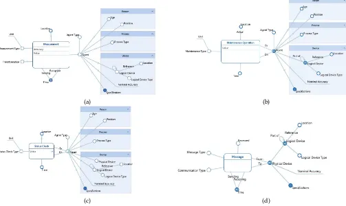
them suitable to be modelled as facts are Measurement,

Maintenance Operation, Status Check, and Message. Before describing these facts one by one, we make a few general observations related to all the schemata:

• The concept of agent is represented as a dimension,

and its specialisation into persons, processes, and devices (as of figure 2) is translated in the DFM as

an additional level Agent Type, whose domain has

values ’Person’, ’Process’, and ’Device’. The levels

that branch from Agent are optional and grouped

into three different sets, one for each type of agent.

Based on the value of Agent Type, only one group

of levels will be meaningful, e.g., if Agent Type =

’Person’, then only Age and Position will take a

value.

• For devices, the domain model shows that one

as-signed device is related to one physical and one log-ical device. So, the agents corresponding to assigned

devices can be grouped by either Logical Device

or Physical Devices. The recursive aggregation of logical devices is represented in the DFM using a

recursive hierarchy (the looping arrow on Logical

Device).

• As with the specialisation ofAgent, the two different

types of logical devices (stationary and mobile) are

differentiated through an additional level called

Log-ical Device Type, while theLocationlevel is optional as it is relevant only for stationary devices.

• The Location level also deserves clarification, as it

can be used in two different ways. The simple way

is that of giving it a simple categorical domain (e.g.,

{’Rooftop’, ’Control’ Room’, ...}) to approximate the geographical positioning of the devices and events. The more complex – but also more expressive – way is ro employ geographical coordinates and

geome-tries that can be fully exploited throughSpatial OLAP

(SOLAP) technologies [22], which allow the user to perform specific OLAP operations tailored for

spatio-temporal data and enablelocation intelligence.

The first schema we discuss is Measurement, shown

in figure 3a. Each measurement event is described by two measures and is defined by six dimensions. The two

mea-sures areValue andAccuracy, which respectively describe

the result of the measurement and its accuracy. Dimension

Measure Type, together with the Unit level, defines the

context of the measurement. For instance, ifMeasure Type

= ’Temperature’ and Unit = ’Celsius Degrees’, then the

meaning of Value is precisely defined as the temperature

in Celsius degrees. TheSensing TimeandReception Time

dimensions define the temporal aspects of the measurement. The remaining dimensions define where the measurement

has been taken (Location), who took it (Agent), and what

kind of processing has been applied to it (Transformation).

TheMaintenanceandStatus Checkschemata, shown in

figures 3b and 3c respectively, are similar toMeasurement.

Here the Maintenance Type and Status Check Type levels

play the same role that Measurement Typeplays in

Mea-surement.

The last schema we discuss isMessage, shown in figure

3d. Unlike from the other facts, messages pertain only to

assigned devices, and so the Agent dimension used in all

the other schemata has been replaced byAssigned Device.

Furthermore, theMessagefact has no measures: a message

either exists or doesn’t. Other modelling choices worth discussing stem from the fact the not all sent messages are actually received, and a communication can be a broadcast where we know who sent the message but not who is supposed to receive it. These two issues are addressed

through the addition of the Communication Type and

Re-ceivedlevels.

(a) (b)

(c) (d)

Fig. 3: Multidimensional schemata for the measurement (a), maintenance (b), status (c), and message (d) events

(i) A successfully delivered message sent from a device

A to a device B is represented as an event with

Communication Type = ’Unicast’, Received = ’True’,

From Physical Device= ’A’, To Physical Device= ’B’, with the corresponding sending and receiving times.

(ii) A failed attempt to deliver a message sent from A

to B is represented as an event withCommunication

Type = ’Unicast’, Received = ’False’, From Physical

Device = ’A’,To Physical Device = ’B’, with only the corresponding sending time.

(iii) A broadcast message sent fromAand received fromB

is represented as in the first example but with

Commu-nication Type= ’Broadcast’. Each message received is represented as a separate event.

(iv) Finally, a broadcast message sent from A but not

re-ceived by any other device is represented as a single

event with Communication Type = ’Broadcast’, From

Physical Device= ’A’, and the corresponding sending time. In this case the receiving device and time are not specified.

4.1 Representation and completeness

For any data warehousing architecture it is important to consider whether it can represent all the data that are anticipated as being collected, and can be extended cleanly to handle unexpected cases – since the goal of the DW is to provide a stable representation unaffected by changes in the operational architecture. How can we provide such assurances for sensor data, where the technology changes rapidly?

We first observe that our domain model captures in many ways the properties of time series and the processes of

their collection, rather than sensor datasetsper se. Within this

broad framework, one may use different measures and lev-els (as discussed in section 2.2) to handle variations. There is already a substantial body of work that can be applied to identifying and extending these elements. One might, for example make use of SensorML as a data model for the individual sensors. As should be clear from the preceeding discussion, however, SensorML in itself is insufficient for sensor data warehousing, as it excludes many elements of context such as maintenance and does not define either a warehousing process or a query process. It is probably better thought of as a component of the data model together with an exchange format.

For sensor modelling purposes, we can map the main SensorML concepts onto the multidimensional schemata

through the Agent attribute. Specifically, the Component

andSystemSensorML concepts correspond to those agents

whoseAgent Type value is ’Device’. Similarly, the

Process-Model andProcessChainconcepts are represented as agents

whose Agent Type value is ’Process’. SensorML also

pro-vides a very generic Event concept, which can be used to

represent any relevant event related to sensors. However, such generic concepts can hardly be used in analytic con-texts without a further modelling step to specialise them

into concepts with a more specific semantics (Status Check,

Maintenance Operation, etc.).

MetadataGroup. While in SensorML these meta-concepts are introduced to facilitate (automatic) processes of resource discovery (which is out of the scope of data warehousing), they can also be useful for analysis purposes. To this end, we

used theSpecificationsattribute in theAgentdimension as a

placeholder that should be replaced with the set of descrip-tive attributes that are relevant to the analysis processes. For example, in the case of sensors for which it is important to know the specific model identifier, one could simply attach to Agent a descriptive attribute namedModel that can be used for filtering and descriptive purposes.

From this discussion it is hopefully clear that (i) our modelling approach is broader than SensorML since it also captures aspects not strictly related to sensors, such as mainteinance; (ii) all the concepts directly modelled in SensorML are also modelled in our approach; and (iii) while for several concepts we adopt the same modelling approach of SensorML (either in direct modelling or meta-modelling), in other cases we chose to directly model concepts that are meta-modelled in SensorML, aimed at making a larger number of semantically well-defined concepts available for analyses to BI users.

5

C

We now present some examples of how these models can be used in practice to carry out several interesting analyses. We consider the cases of air quality monitoring at an industrial facility (see section 5.1), and of landslide risk management in Italy [23] (see section 5.2). These two examples have been chosen due to their rich and varied requirements, and especially for the need to retain and re-interrogate data over different timescales. In both cases we start by discussing the operational requirements for a sensing system in terms of scientific and business challenges, then we describe a possible suite of sensors to address the problem, and finally we show how the data from this sensor network can be modelled in a DW.

5.1 Air quality monitoring

Many large industrial installations operate under tight safe-guarding and permission regimes designed to protect civil-ians near the plants as well as the broader environment. Typically a plant is licensed to emit particular maximum quantities of specific pollutants, and will incur fines or other sanctions for exceeding these limits. Plants will often be required to install systems to monitor their emissions, either directly at point of generation, or indirectly through wider sensing (or both). There may also be further monitoring performed by third-party or regulatory agencies to ensure compliance.

Requirements for air quality monitoring

The main requirements identified for this scenario are listed in table 1. For each requirement we give a brief description and list the related stakeholders and data sources. There are three main types of stakeholders: the facility, the civilians (who are not directly involved with the facility but who can be affected by its emissions), and the regulatory agencies that have the duty of checking whether or not the facility op-erates in respect of environmental norms. Each requirement

can be satisfied by accessing the data stored in the DW and in the data lake. For those requirements that need access to the DW, we also specify which cubes are needed. Note that, for some requirements (denoted with a star in table 1) we list only the main required cube, however other cubes might be useful to get contextual data: for instance for Requirement (1) it could also be useful to know the status of the network to better assess the accuracy of the measurements.

As well as in the obvious detection of leaks and excess emissions, plant managers, regulators, and other agencies have an interest in the long-term relationship of a plant to its environment. One example would be to detect the build-up of pollutants in the local environment even if the plant were operating as licensed. Another would be to implement a market for pollution with a view to encouraging plants to invest to reduce emissions. These scenarios are covered by Requirement (1) and (2) in table 1. Specifically, the first requirement covers the monitoring of air quality in the long term, while the second covers real-time needs where timely alerts are mandatory (such as in case of leaks). Requirement (1) does not need up-to-date data, so it draws from the DW where data are of higher quality. On the other hand, Requirement (2) cannot afford using stale data, thus it draws directly from the data lake, where measurements are stored in real-time and at the finest level of detail.

One challenge often faced in wider sensing is the prlem of attribution: given that a particular situation is ob-served, who was responsible for it? Suppose residents near a plan wake up one morning to discover a fine white powder coating their cars: what is the powder, where did it come from, and who is to blame? Answering these questions requires a combination of direct analysis (what is the powder?) and potentially the fusion of several data streams to determine possible causes: wind direction may exonerate some plants from consideration, for example, but this requires that such data is available, accessible, and reliable. All these challenges are covered by Requirement (3).

Alongside the challenges strictly related to the manage-ment of measuremanage-ments, the facility also needs to monitor the sensor network itself. Indeed, failures of the network must be detected and addressed as quickly as possible for safety reasons. Moreover, failures imply maintenance costs, which should be kept to a minimum. Requirements (4) and (5) re-spectively cover the issues related to the (both real-time and off-line) monitoring of the health status of the network and the issues related to the maintenance operations executed to keep the network running.

Sensing air quality

From the above scientific and business case we can syn-thesise a set of sensors that we need to deploy in order to address a set of scenarios:

• operationalsensing, to ensure that the plant is behav-ing correctly;

• acute event sensing, to detect unexpected emissions as quickly as possible; and

• contextualsensing, to contextualise the other datasets.

TABLE 1: Requirements for the air quality scenario

Name Description Stakeholders Main Data Sources

(1) Air Quality Measurements Quantitatively measure the presence of pollutants in the air in proximity of the facility

Facility, Civilians, Agencies DW (Measurement)* (2) Alerts for High Pollution Detect in a timely fashion the presence of pollutants

in quantities exceeding safe thresholds

Facility, Civilians, Agencies Data Lake

(3) Environmental Conditions Monitor natural phenomena and properties such as wind, humidity, and temperature in proximity of the facility

Facility, Agencies DW (Measurement)*

(4) Network Health Status Detect potentially malfunctioning parts of the net-work

Facility Data Lake, DW (Status Check) (5) Maintenance Operations Keep track of the maintenance operations executed

on the network

Facility, Agencies DW (Maintenance Operation)

chemicals. Such sensors typically require chemical reactions in their operation, which means that their reagents need to be replaced on a regular basis to avoid exhaustion or decalibration through changing chemistry. This addresses the operational and acute scenarios.

To provide context we might also decide to record en-vironmental data (also known as meteorological or “met” data) such as air temperature and pressure, local wind di-rection, local humidity, and precipitation. These time series

are not needed operationally, but might be crucial in post

facto analysis after an incident, where (for example) the chemistry at play might be changed by strong sunlight or an excess of water. They also suggest that we should position sensors differently than we might otherwise, both close to and further from the emission sites (to measure dispersion), and in areas of particular stakeholder interest (wetlands, residential areas, other industrial facilities) to detect potentially dangerous interactions.

Warehousing air quality data

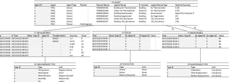
As noted in table 1, the data needed to satisfy the require-ments for this scenario can be drawn from the data lake (for real-time tasks) and from the DW, specifically from cubes

Measurement, Status Check, and Maintenance Operation. We focus on the DW and show a practical example of how the conceptual models of figure 3 can be implemented. Fig-ure 4 shows a basic star schema implementation of the mul-tidimensional schemata proposed in section 4 accompanied by a (fictitious) sample of data. Fact tables and dimension

tables are denoted by prefixesFTandDT, respectively.

We start by commenting the implementation of the

Agent dimension, which is shared by all cubes. Each level (except those not used in this scenario) becomes a column

in tableDT AGENT. The recursive arc onLogical Devicehas

been ignored here as the topology of the sensor network is quite simple and comprises only one layer of sensors. (In case of more complicated topologies, a parent-child table

would be required [4].) LevelR. Locationis used to identify

a generic location but, in more complex networks, it could also be used to refer to specific geographical coordinates.

LevelsProcess TypeandSpecificationshave been omitted

as not necessary here. The sample data forDT AGENT

repre-sent how both devices and persons can be stored together: of course, for each type of agent, only a subset of levels are relevant and thus filled with meaningful values. The remaining dimensions are quite straightforward, especially

the time-related ones andTransformation, which do not need

a separate table and can thus be directly included in the fact tables.

For each multidimensional schema we have a fact table, composed by one column for each dimension and one column for each measure. As noted in table 1 and shown in the sample data in figure 4, Requirements (1) and (2) are

both supported by theMeasurementschema. For instance,

the first two events in tableFT MEASUREMENTrepresent

pollution-related events (Meas. Type ID = 5) computed as

the mean of 10 measurements (Transformation = AVG10)

made by (logical) devices Indoor SO2 Gas Sensor and

Rooftop SO2 Gas Sensor (Agent ID = {5, 6}). The other events are all contextual measurements, such as tempera-ture, wind speed, etc. The remaining fact tables are used to store events respectively related to the status of the network and to the maintenance operations.

To close this section, in figure 5 we show a simple example that combines data from different cubes to per-form an analysis on pollution levels. The pivot table on top shows the weekly average levels of pollution along-side some weather measurements (average wind speed and temperature). Since during the week from 2017/10/16 to 2017/10/22 the sensors outside the facility have measured particularly high levels of pollution, the user might decide to drill-down(i.e., zoom in) on this particular week and on a particular sensor placed outside. The bottom pivot table shows the result of the drill-down that disaggregates the measurements of the chosen sensor on a daily basis. Assum-ing the adoption of a denoisAssum-ing technique, and dependAssum-ing on the adopted data processing policy, noisy measurements could be either tagged or restored. In both cases, the user can determine which data have been affected and evaluate the denoising impact. Furthermore, to check for possible calibration problems, the user also visualises the number of days since the last calibration has been made.

5.2 Landslides risk management

Another interesting scenario is the one presented by

Gior-gettiet alia[23], which describes a wireless sensor network

for the monitoring of landslides. The network, deployed on a rockslide in central Italy, gathered both operational

data (e.g., communication statistics) and measurements of

natural phenomena (e.g., ground movement) in the time

period from February to October 2013.

Requirements for landslides risk management

ge-DT AGENT

Agent ID Agent Agent Type Position Physical Device Logical Device R. Location Logical Device Type Nominal Accuracy

1 TH01 Device - TH000454746 Rooftop Air Thermometer Rooftop Air Thermometer 0.2% 2 TH02 Device - TH000932348 Indoor Air Thermometer Room 01 Air Thermometer 0.2% 3 AN01 Device - AN000328434 Rooftop Anemometer Rooftop Anemometer Speed 5%, Direction 4° 4 HY01 Device - HY000685347 Rooftop Hygrometer Rooftop Air Hygrometer 2%

5 SO01 Device - SO000131220 Indoor SO2Gas Sensor Room 01 SO2Gas Sensor 15%

6 SO02 Device - SO000642337 Rooftop SO2Gas Sensor Rooftop SO2Gas Sensor 15%

7 TE01 Person Field Engineer - - - -

-FT MEASUREMENT

S. Time R. Time Meas. Type ID Agent ID Transformation Accuracy Value

2017/10/13 09:00 2017/10/13 09:00 5 5 AVG10 1.2 8 2017/10/13 09:00 2017/10/13 09:00 5 6 AVG10 14.55 97 2017/10/13 09:00 2017/10/13 09:01 1 1 - 0.028 14 2017/10/13 09:00 2017/10/13 09:02 1 2 - 0.04 20 2017/10/13 09:00 2017/10/13 09:02 2 3 - 0.3 6 2017/10/13 09:00 2017/10/13 09:03 3 3 - 4 90 2017/10/13 09:00 2017/10/13 09:03 4 4 - 0.8 40

FT MAINTENANCE

Time Maint. Type ID By Agent ID On Agent ID Value

2017/10/20 09:00 1 7 5 80 2017/10/20 09:30 1 7 6 80 2017/10/20 13:00 2 7 5 40 2017/10/26 11:00 3 7 1 20

DT MEASUREMENT TYPE

Type ID Type Unit

1 Temperature Degrees Celsius

2 Wind Speed km/h

3 Wind Direction Degrees Azimuth 4 Humidity Relative (%)

5 SO2 μg/m3

DT MAINTENANCE TYPE

Type ID Type Unit

1 Calibration Cost (Euro) 2 Filter Replacement Cost (Euro) 3 Battery Replacement Cost (Euro) FT STATUS

Time Status Type ID By Agent ID On Agent ID Value

2017/10/13 09:00 2 5 5

-2017/10/13 09:01 1 5 5

-2017/10/13 09:00 2 6 6

-2017/10/13 09:01 1 6 6

-2017/10/18 10:00 3 1 1

-DT STATUS TYPE

Type ID Type Unit

1 Asleep None

2 Active None

3 Battery Exhausted None

Fig. 4: Star schema and sample data for the air quality scenario

TABLE 2: Requirements for the landslides scenario

Name Description Stakeholders Main Data Sources

(1) Ground Movements Monitor the behaviour of the landslide Geologists DW (Measurement)* (2) Environmental Conditions Measure natural phenomena and properties such as wind,

temperature, and humidity

Geologists DW (Measurement)* (3) Network Synchronization Gather statistics on the synchronization among the nodes of

the network

Engineers DW (Status Check) (4) Communications Monitor communications between the nodes of the network Engineers DW (Message) (5) Maintenance Operations Keep track of the maintenance operations executed on the

network

Engineers, Geologists DW (Maintenance Operation)

Daily SO2Levels for Week 2017/10/16 and Rooftop SO2 Gas Sensor

Date SO2 Days Since Last Calibration

2017/10/16 135 15

2017/10/17 170 16

2017/10/18 192 17

2017/10/19 205 18

2017/10/20 106 0

2017/10/21 102 1

2017/10/22 98 2

Weekly SO2Levels

Week Location SO2 Wind (km/h) Temperature

2017/10/02 – 2017/10/08 Rooftop 98 7 13

Room 01 11 - 20

2017/10/09 – 2017/10/15 Rooftop 105 9 15

Room 01 13 - 20

2017/10/16 – 2017/10/22 Rooftop 144 4 15

Room 01 16 - 20

drill-down

Fig. 5: A simple analysis performed on air quality data

ologists are mainly interested in the collected measurements and, to better assess their validity, to the history of mainte-nance operations. The engineers are mainly interested in the operational data instead, to check if the network is working as intended.

The main goal of this sensor network is to collect data to observe and analyse landslides. To this end, both ground movement data (Requirement (1)) and other environmental measurements (Requirement (2)) must be taken into ac-count. These data can be used to identify relevant factors causing landslides, thus aiding in preventing and reducing their negative impact.

Similarly to the air quality scenario presented in sec-tion 5.1, during the monitoring campaign the network

it-self was observed to collect operational data. Specifically, the network periodically collected and sent data regarding its synchronization mechanism (Requirement (3)) and the messages exchanged between the nodes (Requirement (4)). These data are crucial to determine if the network is behav-ing as intended: indeed, the network employs adaptive rout-ing strategies designed to cope with harsh environmental conditions (for example foliage, debris, ground movements, and so forth). Finally, maintenance operations (Requirement (5)) must also be recorded to enable efficient management of the network and reduce costs.

Sensing landslide risk data

The sensor network deployed for the scenario described above is composed of 15 wireless nodes each equipped with 3 clinometers, 4 wire extensometers, 2 bar extensometers, and 4 soil hygrometers. One of these nodes acts as a sink that sends data to a remote unit for further elaboration. The sink node is also equipped with a weather station for collwectiong met data. Sensor nodes are equipped with lead-acid batteries and a solar cell.

The logical topology of the network is a tree where the root is the sink node. Each node can send data only to its parent, so the sensed data of a node can reach the sink only through child-parent communications. Note that the network is self-organising and has a dynamically defined topology to improve fault tolerance and adaptability with minimal manual intervention.

FT MESSAGE

S. Time R. Time Communication Message Type Received From P. Device ID To P. Device ID

2013/04/08 09:00 2013/04/08 09:00 Unicast Tilt Meas. Yes 4 2 2013/04/08 09:01 2013/04/08 09:01 Unicast Tilt Meas. Yes 2 1 2013/04/16 16:00 2013/04/16 16:00 Unicast Ext. Meas. Yes 5 3 2013/04/16 16:01 - Unicast Ext. Meas. No 3 1 2013/04/16 16:15 2013/04/16 16:15 Unicast Ext. Meas. Yes 3 1

FT STATUS

Time Status Type By Agent ID On Agent ID Value

2013/04/08 07:00 Sleep 2 2 -2013/04/08 08:58 Association 2 2 -2013/04/08 09:00 Receive 2 2 -2013/04/08 09:01 Transmit 2 2 -2013/04/08 09:02 Sleep 2 2

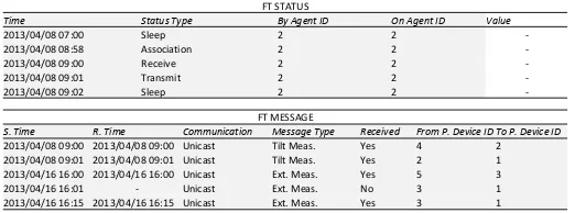
-Fig. 6: Star schema and sample data for the landslide risk management scenario

part of the network. The receive and transmit phases are related to the reception and transmission of data, respec-tively. Finally, to save energy, a node might enter a sleep phase where neither reception nor transmission of data are possible.

Warehousing landslides risk data

As for the air quality case, figure 6 shows a possible rela-tional implementation with some representative data. We

have omitted the implementations of Agentand

Measure-ment since they do not significantly differ from the ones

presented in the previous scenario. In this case we focus on

factsMessageandStatus Check, which are used to support

Requirement (3) and (4).

The synchronisation mechanism described in the previ-ous section is at the core of Requirement (3). As shown in

figure 6 (tableFT STATUS), each phase change is recorded

as a status check event performed by an agent on itself. The type of phase (sleep, association, receive, and transmit) is

represented through theStatus Check Typelevel, while the

Time level marks the beginning of the current phase and

the end of the previous one. Optionally, theValuemeasure

could be used to explicitly denote the duration of each phase.

As for Requirement (4), each packet exchanged between the nodes of the network can be represented by a message

event as shown in figure 6 (table FT MESSAGE).

Specif-ically, the analyses performed in the study presented by

Giorgettiet alia[23] involved the computation of two scores,

thefraction of packets sent(FPS) and thepacket retransmission

rate(PRR). The former is computed as the number of packets

sent from nodeT to nodeR, divided by the total number of

packets sent by R; FPS is thus used to identify which

net-work paths are most (or least) used. The latter score quan-tifies the quality of a given link between two nodes and is computed as the percentage of retransmitted packets. Both scores can be easily computed based on the data contained

in tableFT MESSAGE. Indeed, each event represents either

an attempt of transmitting a packet (Received= ’No’) or a

successful transmission (Received= ’Yes’). To compute FPS

is sufficient to count the number of successful transmission between all pairs of nodes, while for PRR the relevant events that have to be counted are the failed transmissions.

6

C

We have presented a reference architecture and model for constructing DWs of sensor data. We propose such models

as a solution to the challenges posed by the collection and long-term retention and querying of sensor datasets. With-out well-founded data handling, we can have no confidence in the conclusions we draw a long time after the data has been collected, which severely limits the applications and analyses we can support. But without such high-value analyses, many sensor network deployments are financially inviable or scientifically questionable. We therefore believe that the use of data warehousing techniques is a crucial component to the evolving landscape of sensor and IoT systems.

We aimed in this paper to cross-fertilise the fields of sensor networks with contributions coming from the data analysis and big data communities. Although the three fields are perceived as quite closed, the requests from both academics and practitioners for a well-defined, robust, and comprehensive architecture and model are frequently ap-parent. Our experiences in both IoT and “pure” sensing projects show that the adoption of naïve or off-the-shelf solutions reduce analytic capabilities, and such choices, once adopted, are difficult if not impossible to recover from.

Technology for data analysis and big data is evolving fast. Nonetheless the functional architecture proposed as well as the usage of multidimensional cubes are well-established, and for this reason we believe that our proposal can be a starting point for a robustm long-term data analysis solution for sensor systems. We intend in future work to validate these ideas more thoroughly against real-world deployments.

Acknowledgements

The work underlying this paper started as a result of a visit that the third author made to St Andrews in the summer of 2016, and has been partially supported by the UK EPSRC under grant number EP/N007565/1, “Science of Sensor Systems Software”.

R

[1] J. Coutaz, J. Crowley, S. Dobson, and D. Garlan, “Context is key,”

Communications of the ACM, vol. 48, no. 3, pp. 49–53, 2005.

[2] L. Fang and S. Dobson, “Towards data-centric control of sensor

networks through Bayesian dynamic linear modelling,” inProc.

SASO, 2015.

[3] H. Fang, “Managing data lakes in big data era: What’s a data lake

and why has it became popular in data management ecosystem,” inProc. CYBER, 2015, pp. 820–824.

[4] M. Golfarelli and S. Rizzi,Data warehouse design: Modern principles

and methodologies. McGraw-Hill, Inc., 2009.

[5] Z. Huo, M. Mukherjee, L. Shu, Y. Chen, and Z. Zhou,

“Cloud-based data-intensive framework towards fault diagnosis in

large-scale petrochemical plants,” inProc. IWCMC, 2016, pp. 1080–1085.

[6] M. Scriney, M. F. O’Connor, and M. Roantree, “Generating cubes

from smart city web data,” in Proc. ACSW, Geelong, Australia,

2017, pp. 49:1–49:8.

[7] M. Golfarelli, D. Maio, and S. Rizzi, “Conceptual design of data

warehouses from E/R schemes,” inProc. HICSS, vol. 7. IEEE,

1998, pp. 334–343.

[8] M. Golfarelli, S. Graziani, and S. Rizzi, “Starry vault: Automating

multidimensional modeling from data vaults,” in Proc. ADBIS,

2016, pp. 137–151.

[9] O. G. Consortium et al., “OGCR SensorML: Model and XML

encoding standard,” Retrieved from http://www. opengeospatial. org/standards/sensorml, 2014.

[11] T. G. Stavropoulos, D. Vrakas, D. Vlachava, and N. Bassiliades, “Bonsai: a smart building ontology for ambient intelligence,” in

Proc. WIMS, 2012, p. 30.

[12] D. Martin, M. Burstein, J. Hobbs, O. Lassila, D. McDermott, S. McIlraith, S. Narayanan, M. Paolucci, B. Parsia, T. Payne,

et al., “OWL-S: Semantic markup for web services,”W3C member submission, vol. 22, pp. 2007–04, 2004.

[13] F. Cicirelli, G. Fortino, A. Guerrieri, G. Spezzano, and A. Vinci, “Metamodeling of smart environments: from design to imple-mentation,”Advanced Engineering Informatics, vol. 33, pp. 274–284, 2017.

[14] J. Ye, L. Fang, and S. Dobson, “Discovery and recognition

of unknown activities,” in Proceedings of the 2016 ACM

International Joint Conference on Pervasive and Ubiquitous Computing (Ubicomp’16): Adjunct, 2016, pp. 783–792. [Online]. Available: doi://10.1145/2968219.2968288

[15] M. L. L. De Faria, C. E. Cugnasca, and J. R. A. Amazonas, “Insights into IoT data and an innovative DWT-based technique to denoise sensor signals,”IEEE Sensors Journal, vol. 18, no. 1, pp. 237–247, 2018.

[16] M. Zaharia, R. S. Xin, P. Wendell, T. Das, M. Armbrust, A. Dave, X. Meng, J. Rosen, S. Venkataraman, M. J. Franklin,et al., “Apache

spark: A unified engine for big data processing,”Communications

of the ACM, vol. 59, no. 11, pp. 56–65, 2016.

[17] K. Shvachko, H. Kuang, S. Radia, and R. Chansler, “The hadoop distributed file system,” inProc. MSST, 2010, pp. 1–10.

[18] A. Floratou, U. F. Minhas, and F. Özcan, “SQL-on-Hadoop: Full

circle back to shared-nothing database architectures,” PVLDB,

vol. 7, no. 12, pp. 1295–1306, 2014.

[19] P. J. Sadalage and M. Fowler,NoSQL distilled: a brief guide to the

emerging world of polyglot persistence. Pearson Education, 2012. [20] F. Ming, S. Guannan, and L. Shuaishuai, “Research on

multidimen-sional analysis method of drilling information based on Hadoop,” inProc. ICCC. IEEE, 2017, pp. 2319–2322.

[21] S. Russell, P. Norvig, and A. Intelligence, “A modern approach,”

Artificial Intelligence, vol. 25, p. 27, 1995.

[22] S. Rivest, Y. Bédard, M.-J. Proulx, M. Nadeau, F. Hubert, and J. Pastor, “SOLAP technology: Merging business intelligence with geospatial technology for interactive spatio-temporal exploration and analysis of data,”ISPRS, vol. 60, no. 1, pp. 17–33, 2005. [23] A. Giorgetti, M. Lucchi, E. Tavelli, M. Barla, G. Gigli, N. Casagli,