Flocking Control of a Group of Agents Using a
Fuzzy-Logic-Based Attractive/Repulsive Function
Hui Yu, Jigui Jian, Yanjun Shen
Institute of Nonlinear and Complex Systems, China Three Gorges University, Yichang, China E-mail:{yuhui,jiguijian,Shenyj}@ctgu.edu.cn
Received March 5,2010; revised April 7,2010; accepted May 17,2010
Abstract
In this study, a novel procedure is presented for control and analysis of a group of autonomous agents with point mass dynamics achieving flocking motion by using a fuzzy-logic-based attractive/repulsive function. Two cooperative control laws are proposed for a group of autonomous agents to achieve flocking formations related to two different centers (mass center and geometric center) of the flock. The first one is designed for flocking motion guided at mass center and the other for geometric center. A virtual agent is introduced to represent a group objective for tracking purposes. Smooth graph Laplacian is introduced to overcome the difficulties in theoretical analysis. A new fuzzy-logic-based attractive/repulsive function is proposed for separation and cohesion control among agents. The theoretical results are presented to indicate the stability (separation, collision avoidance and velocity matching) of the control systems. Finally, simulation example is demonstrated to validate the theoretical results.
Keywords:Flocking, Cooperative Control, Multi-Agent System, Fuzzy Logic
1. Introduction
A special behavior of large number of interacting dynamic agents called “flocking” has attracted many researchers from diverse fields of scientific and engineering disciplines. Examples of this behavior in the nature include flocks of birds, schools of fish, herds of animals, and colonies of bacteria.
In 1986, Reynolds introduced three heuristic rules that leads to the creation of the first computer animation model of flocking [1]. It should be noticed that these rules are also known as cohesion, separation, and alignment rules respec-tively in the literature. Similar problems have become a major thrust in systems and control theory, in the context of cooperative control, distributed control of multiple vehicles and formation control. A research field which is tightly related to the theme of this paper is that of consensus seek-ing of autonomous multi-agent. In this case, multi-agent achieve consensus if their associated state variables con-verge to a common value [2-5]. In the meantime, an im-portant progression has been achieved on synchronous and/or asynchronous swarm stability analysis [6-8]. Pio-neering works [9-11] on flocking motion of particle sys-tems have properly explained the heuristic rules embedded in Reynolds model. One of the important works in [9-11] is the design of attractive/repulsive potential function. In [12],
Gu and Hu proposed a flocking control algorithm for fixed and switching network of multi-agent respectively, in which the attractive/repulsive potential was designed using fuzzy logic. Stability is analyzed using the classical Lya- punov theory in fixed network and non-smooth analysis in dynamical network, respectively.
In this study, the flocking behaviors of multi-agent sys-tems with point mass dynamics and dynamical network topology are investigated. The major difference or contri-bution compared with previous works, for example [9-12], can be outlined as follows. First of all, the new results are based on more general particle model and the flocking mo-tion is centered at different centers, e.g., mass center and geometric center. Secondly, two new cooperative control laws are proposed such that desired collective behaviors (separation, collision avoidance and velocity matching) can be achieved. Finally, smooth graph Laplacian and smooth attractive/repulsive potential based on fuzzy logic are pro-posed to overcome the difficulties in theoretical analysis and for separation and cohesion control between agents, respectively. In contrast to [12], owing to the design of smooth attractive/repulsive potential based on fuzzy logic and application of smooth graph Laplacian, stability analy-sis both in fixed and dynamical networks can easily con-ducted using classical Lyapunov theory.
2, the problems are formulated based on algebraic graph theory, preliminaries about smooth collective potential function and fuzzy control function are provided. In Sec-tion 3, two flocking control laws based on fuzzy logic are proposed. Stability analysis is given in Section 4. Simula-tion results are provided in SecSimula-tion 5. Finally, concluding remarks are made in Section 6.
2. Problem Formulation and Preliminaries
2.1. System Dynamics
Consider a group of N agents (or particles) moving in an n-dimensional Euclidean space, each has point mass dynamics described by
1 ,
, ,2,
i i i i i i i x v
mv u k v i N
=
= − =
& L
&
(1)
where xi =( ,x x1i i2,L,xin T) ∈¡n is the position vector
of agent i , vi=( ,v vi1 i2,L,vin T) ∈¡n is its velocity
vector, mi >0 is its mass,
1 2
( , , , n T) n
i i i i
u = u u Lu ∈¡
is the control input acting on agent i, ki >0 is the velocity damping gain, and −k vi i is the velocity damp-ing term.
For flocking motion of a group of agents, the control objectives are to design flocking control laws such that:
a) The distances ‖xj−x‖i between any two neighbor
agents are asymptotically convergent to a desired con-stant value d;
b) The velocity vectors vi reach consensus, i.e.,
1 2 N c r
v =v =L=v =v =v , where vc is the velocity vector of the center of a group of agents and vr is the velocity vector of a virtual agent;
c) No collision between agents occurs during the flocking.
The theoretical framework presented in this paper for creation of flocking behavior relies on a number of fun-damental concepts in algebraic graph theory [13] that are described below.
A weighted undirected graph will be used to model the interaction topology among agents. An undirected graph G consists of a set of vertices V={1, 2,L, }N and a set of edgesE= ×V V , where an edge is an unordered pair of distinct vertices inV. In graphG, the ith node represents agent i and a edge denoted as eij or ( , )i j represents an information exchange link between agentiand j. The adjacency matrix A G( )=[aij] of a graph G is a matrix with nonzero elements satisfying the propertyaij ≠ ⇔0 ( , )i j ∈E. Throughout the paper,
for simplicity of notation, we assume aii =0 for all i (or the graphs have no loops). The graph is called weighted whenever the elements of its adjacency matrix are other than just 0 1− elements. Here, weighted un-directed graph is used in this paper. The degree matrix of
G is a diagonal matrix ∆( )G with diagonal elements
1
N j=aij
Σ that are row-sums ofA G( ). The graph Laplacian is defined as ( )L G = ∆( )G A G− ( ). The Laplacian matrix
( )
L G always has a right eigenvector 1N =(1,1,L,1)T associated with eigenvalueλ1=0. A graph G is called
undirected if and only if the adjacency matrix A G( ) is symmetric. The set of neighbors of node i is defined by
{ : 0} { : ( , ) }
i = ∈j aij ≠ = ∈j i j ∈
N V V E (2)
In fixed network topology, agent i can range or communication with a fixed set of neighbors. Therefore, the set Ni is time invariant. However, in dynamical or switching network topology, the set of neighbors of agent i is time-varying due to limited communication.
2.2. Smooth Collective Potential Function
Smooth collective potential function is originally pro-posed in [11]. The following is a brief introduction about it. For more detailed information, the reader is referred to [11].
In order to construct smooth collective potential
func-tion, a map · : 0
n
σ ¡ →¡≥
‖‖ is defined as
2 1
( 1 1)
zσ ε z
ε
= + −
‖‖ ‖‖
with a parameter ε>0. Note that ‖‖zσ is differenti-able everywhere, but ‖‖z is not differentiable atz=0.
Smooth adjacency matrix elements are constructed by using a scalar function ρh( )z that smoothly varies be-tween 0 and 1 . One possible choice is as follows:
(
)
[0, )cos [ ,1]
1 1 1
( ) 1
2
0
h
h
z h
z
z z
otherwise h h
π ρ
= +
∈
∈ −
−
(3)
where h∈(0,1). Using this function, a position-depen- dent adjacency matrix A( )x can be defined asA( )x =[aij( )]x with
( )
(
/ ) [0,1],
ij h j i
a x
=
ρ
‖
x
−
x
‖
σr
σ∈
j i
≠
(4)and position-dependent Laplacian matrix as L( )x =
( ( ))x ( )x
∆A −A , where ( 1, 2, , )
T T T T
N
0
r> denote the interaction range between two agents. The set of neighbors of agent i is defined by
( ) { : }
i x = ∈j ‖xj−xi‖<r
N V .
By the definition of‖‖zσ , the control objective (1) can be expressed as following algebraic constraint:
, ( )
j i i
x −x σ =dσ ∀ ∈j x
‖ ‖ N (5)
wheredσ =‖ ‖dσ.
Given a interaction ranger>0, a neighboring graph ( )x
G can be specified by V and the set of
edges E( )x ={( , )i j ∈ ×V V:‖xj−xi‖<r j, ≠i} , that
clearly depends onx.
A smooth collective potential function has the form:
1 1
( ) ( )
2 i j i j i
V x ψ x x σ
≠
=
∑∑
‖ − ‖where ψ( )z is a smooth pairwise attractive/repulsive potential with a finite cut-off at z=rσ and a global minimum atz=dσ. In order to construct a smooth po-tential functionψ( )z , denote φ( )z = ∇zψ( )z and define this function as:
( )z z ( )z h( /z rσ) ( )z
φ = ∇ψ =ρ ϕ (6)
where ϕ( )z is some function to be designed. Obviously, function φ( )z should vanish for allz≥rσ.
In the next section, the function φ( )z is implemented using fuzzy logic.
2.3. Preliminaries of Fuzzy Control Function
To the best of our knowledge, for flocking control, [12] is the first paper in which attractive/repulsive function is designed using fuzzy logic. In this section, we provide a brief introduction about fuzzy control function [12].
A set of fuzzy logic rules performs a mapping from an inputζ ∈RP to a deterministic control g( )ζ , i.e., fuzzy control function. For the kth dimension state
( 1, 2, , ; 1, 2, , )
k i
x k= L n i= L N , agent i uses states
( ,x xi j) to build a P-dimension vector ζ =
1 2
( ,ζ ζ ,L,ζP) as fuzzy input. The corresponding fuzzy input set isF F1, 2,L,FP. A fuzzy rule between agent i
and agent j can be expressed as: 1
,
1
: IF is AND, L, AND is ,
THEN
l l l
I P P
P
k l l l
ij O P P
P
R F F
g
ζ ζ
θ θ ζ
= = +
∑
where k=1, 2,L, ;n l=1, 2,L,L, L is the number of fuzzy rules.
Use the Gaussian function to define the membership
function of fuzzy setFpl: exp[ 2( )2]
l p p
l l
p p
a F
ζ σ
µ = − − , where
, ( 1, 2, , )
l l p p
a σ p= L P are the mean and variance,
re-spectively. The activation degree of rule Rl is calcu-lated by product operation:
2 1 1
exp[ ].
2( ) l
P P
p p l
l p
p p
a
ζ ξ
σ
= =
−
=
∏
−∑
The crisp output gijk( ),ζ k=1, 2,L, ,n is calculated
by center of area method:
,
1 1
( ) .
L L
k l k l l
ij ij
l l
g ζ ξ g ξ
= =
=
∑
∑
3. Flocking Motion Guided at Mass Center
and/or Geometric Center
In this section, two cooperative control algorithms are developed for flocking guided at mass center and geo-metric center respectively. In flocking motion, each agent applies a control input that consists of four terms:
f c
i i i i i i
u =u +u +uγ +k v (7)
where 1( )
i
f
i x
u = −∇ V x is a gradient-based term and will
be designed using fuzzy logic, uic is a velocity
consen-sus/alignment term, uiγ is a navigation term due to a group objective and k vi i is the velocity damping term.
Similar to [9-11], the velocity consensus/alignment term uic is in the form
( )
( )( )
i
c
i ij j i
j N x
u a x v v
∈
=
∑
− (8)and
( )
( )( )
i
c
i i ij j i
j N x
u m a x v v
∈
=
∑
− (9)for flocking motion guided at mass center and geometric center, respectively. The navigation term uiγ is de-signed in the following form
1 2
1 2
( ) ( )
( , ), , 0.
i i i r i i r
i r r r
u k m x x k m v v
m
f x v k k
m
γ = − − − −
+ > (10)
The pair (x vr, r)∈¡ ¡n× n is the desired state
vec-tor of the group center (mass center or geometric cen-ter). The desired state of the group center can be de-scribed by
( , )
r r
r
r r r
x m v
v f x v
=
=
&
3.1. Fuzzy Attractive/Repulsive Control
For state vector xi , the fuzzy input ζ consists of
, ( )
j i
x −x σ −dσ j∈ x
‖ ‖ N and aij( )x nijk,j∈N( )x ,
where 2 1 k k j i j i k ij x x n x x ε − − =
+‖ ‖ , i.e., P=2 and ζ =(ζ ζ1, 2)
( , ( ) k)
j i ij ij
x x σ dσ a x n
=‖ − ‖ − . The fuzzy output is defined
as
,
2 ( ) , 1, 2, , .
k l l k
ij ij ij
g =θ a x n k= L n
which implies 0 1 0
l l
θ =θ = . A fuzzy rule Rl is then defined as:
, 2 IF xj-xi dσ isFIlTHENgijk l laij( )x nijk
σ − =θ
Therefore, 2 1 1 ( ) ( ) . L l l
k l k
ij ij M ij
l
m
g a x n
ξ θ ζ ξ = = ∑ = ∑
The fuzzy output vector between agent i and j is 2
1 2 1
1
( ) ( , , , ) ( ) ,
L l l
n l
ij ij ij ij ij M ij
l
m
g g g g a x n
ξ θ ζ ξ = = ∑ = = ∑ T L
where 1 2
2
( , , , ) .
1
j i n
ij ij ij ij
j i
x x
n n n n
x x ε − = = + − T L ‖ ‖
Denote the gradient of the attractive/repulsive poten-tial ψ(‖xj−xi‖σ) as:
1 2 1 1 ( ) ( ) L l l l
j i ij L
l
l
x x a x
ζ σ ξ θ ψ ξ = = ∑ ∇ − = ∑ ‖ ‖ and denote 2 1 1 ( ) L l l l
j i L
l
l
x x σ
ξ θ ϕ ξ = = ∑ − = ∑
‖ ‖ , we have
1 1 1 ( ) ( ) ( ) ( ) ( ) ( ) i i
ij ij j i ij
j i ij
j i x
x j i
g a x x x n
x x n
x x x x σ ζ σ ζ σ ζ ϕ ψ ψ ζ ψ = − ∇ − −∇ − ∇ −∇ = = = − ‖ ‖ ‖ ‖ ‖ ‖ ‖ ‖ (12)
Therefore, gradient-based control term can be de-signed as ( ) ( ) ( ) ( ) ( ) ( ) ( ) i i i i f
i x j i ij
j x j x
ij j i ij
j x
u x x g
a x x x n
σ σ ψ ζ ϕ ∈ ∈ ∈ = − ∇ − = = −
∑
∑
∑
‖ ‖ ‖ ‖ N N N (1)3.2. Flocking Control guided at Group Centers
Consider the multi-agent motion relative to the group center xc(the mass centerxmcor geometric centerxgc).
The position and velocity vectors of agent irelative toxcis denoted byx%i = −xi xcandv%i = −vi vc, the collec-tive state vectors of all agents relacollec-tive to xc by
1N c
x%= −x ⊗x and v%= −v 1N⊗vc , where xc =xmc or
gc
x , vc=x&c, ⊗is kronecker product. The mass center of all agents is defined as
1 1
N N
mc i i i
i i
x m x m
= =
=
∑
∑
(14)Note that
1 2
1 2 1
2
( ) ( ) ( , )
( )
( ) ( , )
i
i i i r i i r r r
r
i i i i i mc r
i
i mc r r r
r
m
u k m x x k m v v f x v
m
k m x k m v k m x x
m
k m v v f x v
m
γ = − − − − +
= − − − −
− − +
% % (15)
and due to
1 1 0, 0 N N f c i i i i u u = = = =
∑
∑
, 1 0 N i i i m x = =∑
% , 1 0 N i i i m v = =∑
% , we have1 1
1 2
1
( ) ( ) ( , )
N N
mc i i i
i i
mc r mc r r r
r
v m v m
k x x k v v f x v
m = = = = − − − − +
∑
∑
& &Then, the dynamic of mass center is given by
1 2 1 ( ) ( ) ( ) = , mc mc
mc mc r mc r r r
r x
v k x x k x
v
v v f v
m = − − − − + &
& (16)
Denoteemc =(xTmc−xTr,vmcT −vrT T) , the relative dy-namic of center of mass is given by
mc mc
e& =Ke% (17) where
1 2
0 1
, .
n
K K I K
k k = ⊗ = − − %
We can choose proper control parameters k1>0 and
2 0
k > such that matrix K is Hurwitz stable, and from Lyapunov theory, for given positive matrix 2 2
Q∈¡× , there exists a positive definite matrix P∈¡2 2× , such that:
.
T
K P+PK = −Q (18)
( ) 1 ( ) 2 ( ) ( ) ( )( ) ( ) ( ) ( , ) i i mc i i
ij j i ij
j x
ij j i i i r j x
i
i i r r r i i
r
u u
a x x x n
a x v v k m x x
m
k m v v f x v k v
m σ ϕ ∈ ∈ = = − + − − − − + +
∑
∑
‖ ‖ N N (19) where ,2 1 1 ( ) M Mm m m
j i ij i ij
m m
x x σ
ϕ ξ θ ξ
= =
− =
∑
∑
‖ ‖ .
The geometric center of all agents is defined as
1 1 ( ) N gc i i
x x x
N =
=ave =
∑
(20)Similarly, for geometric center, we propose following control law: ( ) ( ) 1 2 ( ) ( ) ( ) ( ) ( ) ( ) ( , ) i i gc i i
ij i j i ij
j x
ij i j i j x
i
i i r i i r r r i i
r
u u
a x m x x n
a x m v v
m
k m x x k m v v f x v k v
m σ ϕ ∈ ∈ = = − + − − − − − + +
∑
∑
‖ ‖ N N (21)4. Analysis of Stability
In this section, we present our main results for flocking in multi-agent networks with dynamical topology, and conduct stability analysis based on classical Lyapunov theory and LaSalle's invariance principle. In [12], owing to the discontinuity of collective potential function in the case of dynamical topology, stability analysis is done using classical Lyapunov theory in fixed networks and nonsmooth analysis theory, which is difficult to under-stand for engineers in real applications, in dynamical networks, respectively. In our paper, due to the design of smooth collective potential function, in both cases of fixed network and dynamical network, stability analysis can be conducted based on classical Lyapunov theory and LaSalle's invariance principle.
For the collective motion relative to mass centerxmc, define energy function
1 2 3 4
( , ) ( ) ( ) ( ) ( , )
V x v =V x +V x +V v +V x v (22)
where, 1 1 ( ) ( ) 2 1 ( ), 2 j i i j i
j i i j i
V x x x
x x σ σ ψ ψ ≠ ≠ = − = −
∑∑
∑∑
% % ‖ ‖ ‖ ‖2 1 3
1 1 4 1 1 ( ) , ( ) , 2 2 ( , ) ( ) , N N T T
i i i i i i
i i
T
mc n mc
V x k m x x V v m v v
V x v e P I e
= =
= =
= ⊗
∑
% %∑
% %1 0
k > is the parameter of the navigation term.
Applying control law (19) to system (1), following theorem is held to explain the emergence of flocking behaviors of agents guided at center of massxmc.
Theorem 1 Consider a group of agents applying con-trol law (19) with proper selected parameters k k1, 2 >0
satisfying (18) to system (1). Assume that the initial value V x( (0), (0))v is finite. Then, the following state-ments hold.
(i) The solution of system (1) asymptotically con-verges to an equilibrium point (x v*, mc) where
* x a local minima of is V x1( )+V x2( ).
(ii) The velocities of all agents asymptotically con-verge to the velocity of mass centervmc, and the velocity of mass center vmc asymptotically converge to the de-sired velocityvr, i.e., vi →vmc,i=1, 2,L,N v, mc→vr.
(iii) No collision between agents occurs during the flocking.
Proof: First of all, we explain the fact that the energy function V x v( , ) is positive definite.
Obviously, V x V v2( ), 3( ) and V x v4( , ) is positive.
Therefore, the positive definiteness of energy function ( , )
V x v is equivalent to that ofV x1( ). By similar
analy-sis to theorem 1 of [12], ψ(‖x%j−x%‖i σ) can be designed
positive definite by using proper fuzzy rules, i.e., V x1( )
can be designed positive definite.
Secondly, the derivative of the energy function ( , )
V x v is seminegative definite.
1
1 ( ) 1
( ) i ( )
i
N N
T T f
i x j i i i
i j N x i
V x v ψ x x σ v u
= ∈ =
=
∑ ∑
∇ − = −∑
& ‖ ‖ (23)
2 1
1 ( )
N T i i i i
V x k m v x
= =
∑
& % % (24)
Due to 1 0 N i i i m v = =
∑
% , we have3 1
1
( ) ( ) ( ) .
N
T T
n i i
i
V v V x v I v v uγ
=
= − − ⊗ +
∑
& & % L % %
From (15) and note that
1 2
1
[ ( ) ( )
( , )] 0,
N T
i i mc r i mc r
i
i
r r r
v k m x x k m v v
m f x v m = − − − − + =
∑
% We have 1 21 1 1
.
N N N
T T T
i i i i i i i i
i i i
v uγ k m v x k m v v
= = − = − =
∑
%∑
% %∑
% %3 1
2 2
( ) ( ) ( )
( ) ( )
T n T
n
V v V x v I v
V x k v M I v
= − − ⊗
− − ⊗
& & % %
& %L % (25)
where M =diag m m( 1, 2,L,mN). From (17), we have
4( , ) ( )
T
mc n mc
V x v& = −e Q⊗I e (26)
From (23) to (26), we have
1 2 3 4
2
( , ) ( ) ( ) ( ) ( , )
( ) ( )
( ) 0.
T T
n n
T
mc n mc
V x v V x V x V v V x v
v I v k v M I v
e Q I e
= + + +
= − ⊗ − ⊗
− ⊗ ≤
&
% L % % % (27)
Part (i) and part (ii) follow from LaSalle's invariance principle. As V x v&( , ) is seminegative definite, given
{( , ) : ( , ) }
c x v V x v c
Ω = ≤ , Ωc is an invariant set. From
( , )
V x v ≤c, we have
min
2
( n)
c
mc P I
e ≤ λ ⊗
‖ ‖ . Therefore,
both ‖xmc−xr‖ and ‖vmc−vr‖ are bounded. Given the desired state (x vr, r) is bounded and from the defi-nition of xmc and vmc, we know ( , )x v is bounded.
From LaSalle's invariance principle, all states starting
in Ωc converge to the largest invariant set
{( , ) c: ( , ) 0}
S= x v ∈Ω V x v& = . Hence, all states converge to the largest invariant set S={( , )x v ∈Ωc:vi=
, }
mc r mc r
v =v x =x asymptotically, i.e., all agent veloci-ties vi converge to the velocity of center of mass,vmc, and the position and velocity vectors of center of mass,
, mc mc
x v , converge to the desired states, x vr, r, asymp-totically.
Furthermore, in stable state,V x v( , )→V x1( )+V x2( ). There is a equilibrium point at (x v*, mc) where
* x is a local minima ofV x1( )+V x2( ).
Finally, we prove part (iii) by contradiction. Assume there exists a time t= >t1 0 when two distinct agents
,
k l collide, i.e.,x tk( )1 =x tl( )1 . For all t>0, we have
1
1
( ( )) ( )
2 i j i j i
V x t ψ x x σ
≠
=
∑∑
‖ − ‖\{ , } \{ , , }
( ( ) ( ) )
1
( )
2
( ( ) ( ) )
k l
i k l j i k l j i
k l
x t x t
x x
x t x t
σ
σ σ
ψ
ψ ψ
∈ ∈
= −
+ −
≥ −
∑
∑
‖ ‖
‖ ‖
‖ ‖
V V
At t=t1, defining ψ(0) larger than c leads to
1( ( ))1
V x t ≥c, which is in contradiction with the invariant set Ωc. Therefore, no two agents collide at any time
0
t≥ .
Remark: From theorem 1, control objective a) and b) are achieved, but the geometric characterization of local minima x*of V x1( )+V x2( ) is not possible satisfying
the algebraic constraint (5). In [11], the authors pose two conjectures that establish the close relationship between geometric and graph theoretic properties of any local minima of V x1( )+V x2( ) and features of flocks. Based on the conjectures in [11], we can conclude that the local minima x* of V x1( )+V x2( ) is a so-called quasi- α -lattice [11], i.e., − ≤δ ‖xj−x‖i σ − ≤d δ,
0≤δ =dσ, ( , )∀i j ∈E( )x . Obviously, it is very close to the conformation satisfying algebraic constraint (5).
When control laws (21) applied to system (1), similar theorem is established to explain the emergence of flocking behavior of agents guided at geometric center.
For the collective motion relative to geometric cen-terxgc, define energy function
1 2 3 4
( , ) ( ) ( ) ( ) ( , )
U x v =V x +U x +U v +V x v
Where
1 2 1
1
1 1
( ) ( ), ( ) ,
2 2
N T
j i i i
i j i i
V x ψ x x σ U x k x x
≠ =
=
∑∑
‖ − ‖ =∑
% %3 4
1 1
( ) , ( , ) ( )
2
N
T T
i i gc n gc
i
U v v v V x v e P I e
=
=
∑
% % = ⊗ , k1>0 isthe parameter of the navigation term,
( T T, T T T)
gc gc r gc r
e = x −x v −v .
We have following theorem.
Theorem 2 Consider a group of agents applying con-trol law (21) with proper selected parameters k k1, 2 >0
satisfying (18) to system (1). Assume that the initial valueU x( (0), (0))v is finite. Then, the following state-ments hold.
1) The solution of system (1) asymptotically con-verges to an equilibrium point (x v*, gc) where
* x a
local minima of isV x1( )+U2( )x .
2) The velocities of all agents asymptotically converge to the velocity of geometric centervgc, and the velocity
of geometric center vgc asymptotically converge to the
desired velocity vr , i.e., vi →vgc, i=1, 2,L,N,
gc r
v →v .
3) No collision between agents occurs during the flocking.
Proof: The proof of this theorem is similar to that of theorem 1.
5. Simulation
simulated in 2-dimentional space. The following pa-rameters were fixed throughout the simulation:
2, 1.2 , 0.5
d= r= d ε = , and h=0.3 for ρh( )z . Eight fuzzy sets are designed for the fuzzy control in-put‖xj−xi‖−dσ. They are LN, N, SN, Z, SP, P, LP,
and PP as shown in Figure 1. Eight fuzzy rules are de-signed as follows:
IF ‖xj−xi‖σ −dσ is LN THEN
,1
90 ( / )
k k
ij h j i ij
g = − ρ ‖x −x‖σ r nσ ; IF ‖xj−xi‖σ −dσ is N THEN
,2
80 ( / )
k k
ij h j i ij
g = − ρ ‖x −x‖σ r nσ ;
IF ‖xj−xi‖σ −dσ is SN THEN
,3
50 ( / )
k k
ij h j i ij
g = − ρ ‖x −x‖σ r nσ ;
IF ‖xj−xi‖σ −dσ is Z THENgijk,4 =0;
IF ‖xj−xi‖σ −dσ is SP THEN
,5
0.5 ( / )
k k
ij h j i ij
g = ρ ‖x −x‖σ r nσ ; IF ‖xj−xi‖σ −dσ is P THEN
,6
( / )
k k
ij h j i ij
g =ρ ‖x −x‖σ r nσ ;
IF ‖xj−xi‖σ −dσ is LP THEN
,7
1.5 ( / )
k k
ij h j i ij
g = ρ ‖x −x‖σ r nσ ; IF ‖xj−xi‖σ −dσ is PP THEN
,8
2 ( / )
k k
ij h j i ij
g = ρ ‖x −x‖σ r nσ .
Control parameters k k1, 2 are selected to be k1=
2 1
k = . The two eigenvalues of matrix 0 1
1 1
K= − −
are −05000 08660+ i and −05000 08660− i. Therefore, matrix K is Hurwitzstable. Let Q=I2, using Matlab
command lyap(K,Q), we obtain positive definite matrix
1.5 0.5
0.5 1
P= − −
[image:7.595.349.499.225.356.2] .
Figure 1. Fuzzy membership function.
Simulation is calculated within 20 seconds time by using Matlab Simulink. In addition, the position of each agent is marked with a right triangle sign.
Figures 2 to 5 show the simulation results within 2-D flocking using control law (19) for 50 agents. Figures 2 to
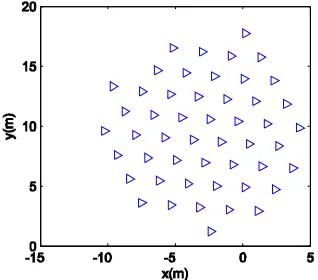
4 show snapshots of 2-D flocking at time t=0, 4.3495, and 20 (sec). The initial position and initial velocity coordinates were uniformly chosen in the random do-main of [0, 3] [0, 3]× and[0,1] [0,1]× , respectively. The mass of each agent was also uniformly chosen in a random domain of [0.5, 1.5]. A steady configuration was formed
[image:7.595.341.501.387.531.2]Figure 2. Initial positions of 50 agents.
Figure 3. Configuration of 50 agents at t = 4.3495 (sec).
[image:7.595.60.256.531.707.2] [image:7.595.344.503.562.702.2]Figure 5. Position-dependent neighboring graph at t = 20 (sec).
Figure 6. Velocities of 50 agents along x-axis and y-axis respectively.
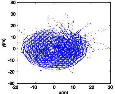
Figure 7. Trajectories of all agents within 20 (sec) time.
as shown in Figure 4 and maintained thereafter. A vir-tual agent
( ) (10 sin(03 ),10 cos(03 )) ,T
r
x t = t t
( ) (3cos(03 ), 3sin(03 ))T r
v t = t − t
was used for this example. For highly disconnected neighboring graph G( )x in initial state, Figure 5 shows the connected neighboring graph G( )x corresponding to the final configuration. Figure 6 shows velocity match-ing is achieved along x-axis and y-axis respectively.
Figure 7 shows the trajectories of all agents within 20(sec) simulation time and the cohesive behaviors. The simulation demonstration with control law (21) was similar to that conducted by control laws (19), and therefore is not necessarily repeated here.
6. Conclusions
This paper establishes a theoretical framework for design and analysis of flocking control algorithms using a fuzzy-logic-based attractive/repulsive potential function for multiple agent networks with dynamical topology. Two cooperative control laws have been proposed for a group of autonomous agents to achieve flocking motion relative to different centers (mass center and geometric center). A virtual agent is introduced to represent a group objective for tracking purposes. Smooth Laplacian and smooth fuzzy-logic-based attractive/repulsive potential are proposed to overcome the difficulties in stability analysis. Simulation results validated the theoretical re-sults.
7. Acknowledgements
This paper is supported in part by Hubei Provincial Natu-ral Science Foundation under the grant 2008CDB316, Natural Science Research Project of Hubei Provincial Department of Education under the grant D20101201, and Scientific Innovation Team Project of Hubei Provin-cial College under the grant T200809.
8. References
[1] C. W. Reynolds, “Flocks, Herds, and Schools: A Distrib-uted Behavioral Model,” Computer Graphics (ACM SIG-GRAPH '87 Conference Proceedings), Vol. 21, No. 4, 1987, pp. 25-34.
[2] R. Olfati-Saber and R. M. Murray, “Consensus Problems in Networks of Agents with Switching Topology and Time-Delays,” IEEE Transactions on Automatic Control, Vol. 49, No. 9, September 2004, pp. 101-115.
[3] A. Jadbabaie, J. Lin and S. A. Morse, “Coordination of Groups of Mobile Agents Using Nearest Neighbor Rules,” IEEE Transactions on Automatic Control, Vol. 48, No. 6, June 2003, pp. 988-1001.
[4] W. Ren and R. Beard, “Consensus Seeking in Multi- Agent Systems Using Dynamically Changing Interaction Topologies,” IEEE Transactions on Automatic Control, Vol. 50, No. 5, May 2005, pp. 655-661.
[image:8.595.92.254.71.228.2] [image:8.595.76.255.267.427.2] [image:8.595.79.264.468.619.2]Time-Dependent Communication Links,” IEEE Transac- tions On Automatic Control, Vol. 50, No. 2, February 2005, pp. 169-182.
[6] Y. Liu, K. M. Passino and M. M. Polycarpou, “Stability analysis of M-dimensional Asynchronous Swarms with a Fixed Communication Topology,” IEEE Transactions on Automatic Control, Vol. 48, No. 1, Juanary 2003, pp.76- 95.
[7] Y. Liu, K. M. Passino and M. M. Polycarpou, “Stability Analysis of One-Dimensional Asynchronous Swarms,” IEEE Transactions on Automatic Control, Vol. 48, No. 10, October 2003, pp. 1848-1854.
[8] V. Gazi and K. M. Passino, “Stability Analysis of Swarms,” IEEE Transactions on Automatic Control, Vol. 48, No. 4, April 2003, pp. 692-697.
[9] H. G. Tanner, A. Jadbabaie and G. J. Pappas, “Stable Flocking of Mobile Agents, Part I: Fixed Topology,” The
42nd IEEE Conference on Decision and Control, Maui, December 2003, pp. 2010-2015.
[10] H. G. Tanner, A. Jadbabaie and G. J. Pappas, “Stable Flocking of Mobile Agents, Part II: Dynamic Topology,” The 42nd IEEE Conference on Decision and Control, Maui, December 2003, pp. 2016-2021.
[11] R. Olfati-Saber, “Flocking for Multi-Agent Dynamic Systems: Algorithms and Theory,” IEEE Transactions on Automatic Control, Vol. 51, No. 3, March 2006, pp. 401-420.
[12] D. Gu and H. Hu, “Using Fuzzy Logic to Design Separation Function in Flocking Algorithms,” IEEE Transactions on Fuzzy Systems, Vol. 16, No. 4, August 2008, pp. 826-838.