The stellar to halo mass relation of GAMA galaxies from 100 deg2 of KiDS weak lensing data

Edo van Uitert,

Marcello Cacciato,

Henk Hoekstra,

Margot Brouwer,

Crist´obal Sif´on,

Massimo Viola,

Ivan Baldry,

Joss Bland-Hawthorn,

Sarah Brough,

M. J. I. Brown,

Ami Choi,

Simon P. Driver,

Thomas Erben,

Catherine Heymans,

Hendrik Hildebrandt,

Benjamin Joachimi,

Konrad Kuijken,

Jochen Liske,

Jon Loveday,

John McFarland,

Lance Miller,

Reiko Nakajima,

John Peacock,

Mario Radovich,

A. S. G. Robotham,

Peter Schneider,

Gert Sikkema,

Edward N. Taylor

and Gijs Verdoes Kleijn

Affiliations are listed at the end of the paper

Accepted 2016 March 26. Received 2016 March 24; in original form 2016 January 22

A B S T R A C T

We study the stellar-to-halo mass relation of central galaxies in the range 9.7<log₁₀(M∗/h−2M)<11.7 and z < 0.4, obtained from a combined analysis of the Kilo Degree Survey (KiDS) and the Galaxy And Mass Assembly (GAMA) survey. We use ∼100 deg2 _{of KiDS data to study the lensing signal around galaxies for which} spec-troscopic redshifts and stellar masses were determined by GAMA. We show that lensing alone results in poor constraints on the stellar-to-halo mass relation due to a degeneracy between the satellite fraction and the halo mass, which is lifted when we simultaneously fit the stellar mass function. AtM_∗>5×1010h−2M, the stellar mass increases with halo mass as∼M_h0.25. The ratio of dark matter to stellar mass has a minimum at a halo mass of 8×1011_h−1_M with a value ofMh/M∗=56+16−10[h]. We also use the GAMA group catalogue to select centrals and satellites in groups with five or more members, which trace regions in space where the local matter density is higher than average, and determine for the first time the stellar-to-halo mass relation in these denser environments. We find no significant differences compared to the relation from the full sample, which suggests that the stellar-to-halo mass relation does not vary strongly with local density. Furthermore, we find that the stellar-to-halo mass relation of central galaxies can also be obtained by modelling the lensing signal and stellar mass function of satellite galaxies only, which shows that the assumptions to model the satellite contribution in the halo model do not significantly bias the stellar-to-halo mass relation. Finally, we show that the combination of weak lensing with the stellar mass function can be used to test the purity of group catalogues.

Key words: gravitational lensing: weak – methods: observational – galaxies: groups: general – galaxies: haloes – galaxies: luminosity function, mass function.

1 I N T R O D U C T I O N

Galaxies form and evolve in dark matter haloes. Larger haloes at-tract on average more baryons and host larger, more massive galax-ies. The exact relation between the baryonic properties of galaxies and their dark matter haloes is complex, however, as various astro-physical processes are involved. These include supernova and AGN

_{E-mail:vuitert@ucl.ac.uk}

feedback (see e.g. Benson2010), whose relative importances gen-erally depend on halo mass in a way that is not accurately known, but environmental effects also play an important role. Measuring projections of these relations, such as the stellar-to-halo mass re-lation, helps us to gain insight into these processes and their mass dependences, and provides valuable references for comparisons for numerical simulations that model galaxy formation and evolution (e.g. Munshi et al.2013; Kannan et al.2014).

matching (e.g. Behroozi, Conroy & Wechsler2010; Moster, Naab & White2013) or galaxy clustering (e.g. Wake et al.2011; Guo et al.2014), which can only be interpreted within a cosmological framework (e.g. CDM). Satellite kinematics offer a direct way to measure halo mass (e.g. Norberg, Frenk & Cole2008; Wojtak & Mamon 2013), but this approach is relatively expensive as it requires spectroscopy for large samples of satellites. Weak gravita-tional lensing offers another powerful method that enables average halo mass measurements for ensembles of galaxies (e.g. Mandel-baum et al.2006; Velander et al.2014). Recently, various groups have combined different probes (e.g. Leauthaud et al.2012; Coupon et al.2015), which enable more stringent constraints on the stellar-to-halo mass relation by breaking degeneracies between model pa-rameters. A coherent picture is emerging from these studies: the stellar-to-halo mass relation of central galaxies can be described by a double power law, with a transition at a pivot mass where the ac-cumulated star formation has been most efficient. At higher masses, AGN feedback is thought to suppress star formation, while at lower masses, supernova feedback suppresses it. This pivot mass coin-cides with the location where the stellar mass growth in galaxies turns from beingin situdominated to merger dominated (Robotham et al.2014).

Most galaxies can be roughly divided into two classes, i.e. red, ‘early types’ whose star formation has been quenched, and blue, ‘late types’ that are actively forming stars. These are also crudely related to different environments and morphologies. The differences in their appearances point at different formation histories. Their stellar-to-halo mass relations may contain information of the under-lying physical processes that caused these differences. Hence it is natural to measure the stellar-to-halo mass relations of red and blue galaxies separately (e.g. Mandelbaum et al.2006; More et al.2011; van Uitert et al.2011; Tinker et al.2013; Wojtak & Mamon2013; Velander et al.2014; Hudson et al.2015). The main result of the aforementioned studies is that at stellar masses below∼1011_M

, red and blue galaxies that are centrals (i.e. not a satellite of a larger system) reside in haloes with comparable masses. At higher stellar masses, the halo masses of red galaxies are larger at low redshift, but smaller at high redshift at a given stellar mass. Tinker et al. (2013) interpret this similarity in halo mass at the low-mass end as evidence that these red galaxies have only recently been quenched; the difference at the high-mass end is interpreted as evidence that blue galaxies have a relatively larger stellar mass growth in recent times, compared to red galaxies.

As red galaxies preferentially reside in dense environments such as galaxy groups and clusters, it appears that local density is the main driver behind the variation of the stellar-to-halo mass relation, and that the change in colour is simply a consequence of quench-ing, as was already hypothesized in Mandelbaum et al. (2006). This scenario could be verified by measuring the stellar-to-halo mass re-lation for galaxies in different environments. This requires a galaxy catalogue including stellar masses and environmental information, plus a method to measure masses. Weak gravitational lensing of-fers a particularly attractive way of measuring average halo masses of samples of galaxies, as it measures the total projected matter density along the line of sight, without any assumption about the physical state of the matter, out to scales that are inaccessible to other gravitational probes.

These conditions are provided by combining two surveys: the Kilo Degree Survey (KiDS) and the Galaxy And Mass Assembly (GAMA) survey. GAMA is a spectroscopic survey for galaxies withr< 19.8 that is highly complete (Driver et al.2009,2011; Liske et al.2015), facilitating the construction of a reliable group

catalogue (Robotham et al.2011). GAMA is completely covered by the KiDS survey (de Jong et al.2013), an ongoing weak lensing survey which will eventually cover 1500 deg2_{of sky in theugri}

-bands. In this work, we study the lensing signal around∼100 000 GAMA galaxies using sources from the∼100 deg2_{of KiDS imaging}

data overlapping with the GAMA survey from the first and second publicly available KiDS-DR1/2 data release (Kuijken et al.2015).

The outline of this paper is as follows. In Section 2 we describe the data reduction and lensing analysis, and introduce the halo model that we fit to our data. The stellar-to-halo mass relation of the full sample is presented in Section 3. In Section 4, we measure this rela-tion for centrals and satellites in groups with a multiplicityNfof≥5.

We conclude in Section 5. Throughout the paper we assume aPlanck

cosmology (Planck Collaboration et al.2014) withσ8 = 0.829,

=0.685,M=0.315,bh2=0.02205 andns=0.9603. Halo

masses are defined asMh≡4π(200 ¯ρm)R2003 /3, withR200the

ra-dius of a sphere that encompasses an average density of 200 times the comoving matter density, ¯ρm=8.74·1010h2MMpc−3, at the

redshift of the lens. All distances quoted are in comoving (rather than physical) units unless explicitly stated otherwise.

2 A N A LY S I S

2.1 KiDS

To study the weak-lensing signal around galaxies, we use the shape and photometric redshift catalogues from the Kilo Degree Survey (KiDS; Kuijken et al.2015). KiDS is a large optical imaging survey which will cover 1500 deg2_{inu,g,randito magnitude limits of}

24.2, 25.1, 24.9 and 23.7 (5σ in a 2 arcsec aperture), respectively. Photometry in five infrared bands of the same area will become available from the VISTA Kilo-degree Infrared Galaxy (VIKING) survey (Edge et al.2013). The optical observations are carried out with the VLT Survey Telescope (VST) using the 1 deg2 _imager

OmegaCAM, which consists of 32 CCDs of 2048×4096 pixels each and has a pixel size of 0.214 arcsec. In this paper, weak lensing re-sults are based on observations of 109 KiDS tiles1_{that overlap with}

the GAMA survey, and have been covered in all four optical bands and released to ESO as part of the first and second KiDS-DR1/2 data releases. The effective area after accounting for masks and overlaps between tiles is 75.1 square degrees. The image reduction and the astrometric and photometric reduction use the ASTRO-WISE

pipeline (McFarland et al.2013); details of the resulting astromet-ric and photometastromet-ric accuracy can be found in de Jong et al. (2015). Photometric redshifts have been derived with BPZ (Ben´ıtez2000; Hildebrandt et al.2012), after correcting the magnitudes in the op-tical bands for seeing differences by homogenising the photometry (Kuijken et al.2015). The photometric redshifts are reliable in the redshift range 0.005< zB<1.2, withzBbeing the location where

the posterior redshift probability distribution has its maximum, and have a typical outlier rate of<5 per cent atzB< 0.8 and a

red-shift scatter of 0.05 (see section 4.4 in Kuijken et al.2015). In the lensing analysis, we use the full photometric redshift probability distributions.

Shear measurements are performed in ther-band, which has been observed under stringent seeing requirements (<0.8 arcsec). Ther -band is separately reduced with the well-tested THELI pipeline (Erben et al.2005,2009), following procedures very similar to the

is better than the current statistical uncertainties, as is shown by a number of systematics tests in Kuijken et al. (2015). Shear esti-mates are obtained using all source galaxies in unmasked areas with a non-zerolensfit weight and for which the peak of the posterior redshift distribution is in the range 0.005< zB<1.2. The

corre-sponding effective source number density is 5.98 arcmin−2_(using

the definition of Heymans et al.2012, which differs from the one adopted in Chang et al.2013, as discussed in Kuijken et al.2015).

2.2 GAMA

The GAMA survey (Driver et al.2009,2011; Liske et al.2015) is a highly complete optical spectroscopic survey that targets galaxies withr<19.8 over roughly 286 deg2_{. In this work, we make use of}

the G3_{Cv7 group catalogue and version 16 of the stellar mass}

cata-logue, which contain∼180 000 objects, divided into three separate 12×5 deg2_{patches that completely overlap with the northern stripe}

of KiDS. We use the subset of∼100 000 objects that overlaps with the 75.1 deg2_{from the KiDS-DR1/2.}

Stellar masses of GAMA galaxies have been estimated in Tay-lor et al. (2011). In short, stellar population synthesis models from Bruzual & Charlot (2003) that assume a Chabrier (2003) Initial Mass Function (IMF) are fit to theugriz-photometry from SDSS. NIR photometry from VIKING is used when the rest-frame wave-length is less than 11 000 Å. To account for flux outside the AUTO aperture used for the spectral energy distributions (SEDs), an aper-ture correction is applied using the fluxscale parameter. This pa-rameter defines the ratio between ther-band (AUTO) aperture flux and the totalr-band flux determined from fitting a S´ersic profile out to 10 effective radii (Kelvin et al.2012). The stellar masses do not include the contribution from stellar remnants. The stellar mass errors are∼0.1 dex and are dominated by a magnitude error floor of 0.05 mag, which is added in quadrature to all magnitude errors, thus allowing for systematic differences in the photometry between the different bands. The random errors on the stellar masses are therefore even smaller, and we ignore them in the remainder of this work. Systematic errors due to e.g. the choice of the IMF are not included in the error budget; their expected magnitude is also

∼0.1 dex.

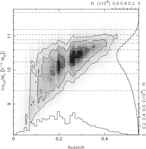
The distribution of stellar mass versus redshift of all GAMA galaxies in the KiDS footprint is shown in Fig.1. This figure shows that the GAMA catalogue contains galaxies with redshifts up to z 0.5. Furthermore, bright (massive) galaxies reside at higher redshifts, as expected for a flux-limited survey. Note that the appar-ent lack of galaxies more massive than a few times 1010_h−2_M

atz <0.2 is a consequence of plotting redshift on the horizontal axis instead of bins of equal comoving volume. The bins at low redshift contain less volume and therefore have fewer galaxies (for a constant number density). It is not a selection effect.

We use the group properties of the G3_{C catalogue (Robotham}

et al.2011) to select galaxies in dense environments. Groups are found using an adaptive friends-of-friends algorithm, linking galax-ies based on their projected and line-of-sight separations. The algo-rithm has been tested on mock catalogues, and the global properties, such as the total number of groups, are well recovered. Version 7 of the group catalogue, which we use in this work, consists of nearly

Figure 1. Spectroscopic redshift versus stellar mass of the GAMA galax-ies in the KiDS overlap. The density contours are drawn at 0.5, 0.25 and 0.125 times the maximum density in this plane. The total density of GAMA galaxies as a function of redshift and stellar mass are shown by the his-tograms on thex- andy-axes, respectively. The dashed lines indicate the mass bins of the lenses.

24 000 groups with over∼70 000 group members. The catalogue contains group membership lists and various estimates for the group centre, as well as group velocity dispersions, group sizes and esti-mated halo masses. We limit ourselves to groups with a multiplicity

Nfof≥5, because groups with fewer members are more strongly

affected by interlopers, as a comparison with mock data has shown (Robotham et al.2011). We refer to these groups as ‘rich’ groups. We assume that the brightest2_{group galaxy is the central galaxy,}

while fainter group members are referred to as satellites. An alter-native procedure to select the central galaxy is to iteratively remove group members that are furthest away from the group centre of light. As the two definitions only differ for a few per cent of the groups and the lensing signals are statistically indistinguishable (see ap-pendix A of Viola et al.2015), we do not investigate this further and adopt the brightest group galaxy as the central throughout. To verify that these ‘rich’ groups trace dense environments, we match the G3_{C catalogue to the environmental classification catalogue of}

Eardley et al. (2015), who uses a tidal tensor prescription to distin-guish between four different environments: voids, sheets, filaments and knots. Using the classification that is based on the 4h−1_Mpc

smoothing scale, we find that 76 per cent of the centrals of groups withNfof≥5 reside in filaments and knots, compared to 49 per cent

of the full GAMA catalogue, which shows theNfof≥5 groups form

a crude tracer of dense regions.

Note that both the stellar mass catalogue and the GAMA group catalogue were derived with slightly different cosmological pa-rameters: Taylor et al. (2011) used (, M, h)=(0.7,0.3,0.7) and

2_{This is based on SDSSr-band Petrosian magnitudes with a global (k+e}

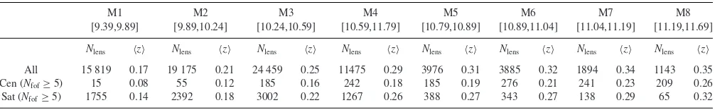
Table 1. Number of lenses and mean lens redshift of all lens samples used in this work. The stellar mass ranges that are indicated correspond to the log10of

the stellar masses and are in units log10(h−2M). The ‘All’ sample contains all GAMA galaxies that overlap with KiDS-DR1/2, while ‘Cen’ and ‘Sat’ refers

to the samples that only contain the centrals and satellites in GAMA groups with a multiplicity Nfof≥5.

M1 M2 M3 M4 M5 M6 M7 M8

[9.39,9.89] [9.89,10.24] [10.24,10.59] [10.59,11.79] [10.79,10.89] [10.89,11.04] [11.04,11.19] [11.19,11.69] Nlens z Nlens z Nlens z Nlens z Nlens z Nlens z Nlens z Nlens z

All 15 819 0.17 19 175 0.21 24 459 0.25 11475 0.29 3976 0.31 3885 0.32 1894 0.34 1143 0.35

Cen (Nfof≥5) 15 0.08 55 0.12 185 0.16 242 0.18 185 0.19 276 0.21 241 0.23 209 0.26

Sat (Nfof≥5) 1755 0.14 2392 0.18 3002 0.22 1267 0.26 388 0.27 343 0.27 138 0.29 65 0.32

Robotham et al. (2011) used (, M, h)=(0.75,0.25,1.0) in order

to match the Millennium Simulation mocks. We accounted for the difference inh, but not in andM, because the lensing signal

at low redshift depends only weakly on these parameters and this should not impact our results.

The current lensing catalogues in combination with these GAMA catalogues have already been analysed by Viola et al. (2015), where the main focus was GAMA group properties, and by Sif´on et al. (2015), where the masses of satellites in groups were derived. Here, we aim at a broader scope, as we measure the stellar-to-halo mass relation over two orders of magnitude in halo mass. Studying the centrals and satellites in ‘rich’ groups supplies us with the first observational limits on whether the stellar-to-halo mass relation changes in dense environments.

2.3 Lensing signal

Weak lensing induces a small distortion of the images of background galaxies. Since the lensing signal of individual galaxies is generally too weak to be detected due to the low number density of background galaxies in wide-field surveys, it is common practice to average the signal around many (similar) lens galaxies. In the regime where the surface mass density is sufficiently small, the lensing signal can be approximated by averaging the tangential projection of the ellipticities of background (source) galaxies, the tangential shear:

γt(R)=

(R) crit ,

(1)

with (R)=¯(< R)−¯(R) the difference between the mean projected surface mass density inside a projected radiusRand the surface density atR, andcritthe critical surface mass density:

crit=

c2

4πG DS DLDLS

, (2)

withDLandDSthe angular diameter distance from the observer to the lens and source, respectively, andDLSthe distance between the lens and source. For each lens–source pair we compute 1/critby

integrating over the redshift probability distribution of the source. We have not computed the error oncritand propagated it in the

analysis. This would require knowledge on the error on the redshift probability distribution of the sources, which is not available. How-ever, for lenses and sources that are well separated in redshift, as is the case here, the lensing efficiencyDLS/DSis not very sensitive to details of the source redshift distribution. Hence we expect that the error oncritcan be safely ignored in our analysis.

The actual measurements of the excess surface density profiles are performed using the same methodology outlined in section 3.3 of Viola et al. (2015). The covariance between the radial bins of the lensing measurements is derived analytically, as discussed in section 3.4 of Viola et al. (2015). We have also computed the covariance

ma-trix using bootstrapping techniques and found very similar results in the radial range of interest.

We group GAMA galaxies in stellar mass bins and measure their average lensing signals. The bin ranges were chosen following two criteria. First, we aimed for a roughly equal lensing signal-to-noise ratio of∼15 per bin. Secondly, we adopted a maximum bin width of 0.5 dex. To determine the signal-to-noise ratio, we fitted a singular isothermal sphere (SIS) to the average lensing signal and determined the ratio of the amplitude of the SIS to its error. The adopted bin ranges are listed in Table1, as well as the number of lenses and their average redshift; the average is shown in Fig.2. We note, however, that our conclusions do not depend on the choice of binning.

2.4 The halo model

The halo model (Seljak2000; Cooray & Sheth2002) has become a standard method to interpret weak lensing data. The implementation we employ here is similar to the one described in van den Bosch et al. (2013) and has been successfully applied to weak lensing measurements in Cacciato, van Uitert & Hoekstra (2014), van Uitert et al. (2015), and to weak lensing and galaxy clustering data in Cacciato et al. (2013). We provide a description of the model here, as we have made a number of modifications.

In the halo model, all galaxies are assumed to reside in spher-ical dark matter haloes. Using a prescription for the way galaxies occupy dark matter haloes, as well as for the matter density pro-file, abundance and clustering of haloes, one can predict the surface mass density (and thus the lensing signal) correlated with galaxies in a statistical manner:

(R)=ρ¯m

ωS

0

ξgm(r)dω, (3)

withξgm(r) the galaxy-matter cross-correlation,ωthe comoving

distance from the observer andωS the comoving distance to the source. For small separations, R≈ωLθ, with ωL the comoving distance to the lens andθ the angular separation from the lens. The three-dimensional comoving distance r is related to ω via r2_=(ω

L·θ)2+(ω−ωL)2. The integral is computed along the line of sight.

As the computation of ξgm(r) generally requires convolutions

in real space, it is convenient to express the relevant quantities in Fourier-space where these operations become multiplications. ξgm(r) is related to the galaxy-matter power spectrum,Pgm(k, z),

via

ξgm(r, z)=

1 2π2

_∞

0

Pgm(k, z)

sinkr kr k

2

dk, (4)

withkthe wavenumber. On small physical scales, the main contribu-tion toPgm(k,z) comes from the halo in which a galaxy resides (the

Figure 2. Excess surface mass density profile of GAMA galaxies measured as a function of projected (comoving) separation from the lens, selected in various stellar mass bins, measured using the source galaxies from KiDS. The dashed red line indicates the best-fitting halo model, obtained from fitting the lensing signal only. The solid green line is the best-fitting halo model for the combined fit to the weak lensing signal and the stellar mass function, the orange area indicates the 1σmodel uncertainty regime of this fit. The stellar mass ranges that are indicated correspond to the log10of the stellar masses and are in units

log10(h−2M).

comes from neighbouring haloes (the two-halo term). Additionally, the halo model distinguishes between two galaxy types, i.e. centrals and satellites. Centrals reside in the centre of a main halo, while satellites reside in subhaloes that are embedded in larger haloes. Their power spectra are different and computed separately. Hence one has

Pgm(k)=Pcm1h(k)+P 1h sm(k)+P

2h cm(k)+P

2h

sm(k), (5)

withP1h cm(k) (P

1h

sm(k)) the one-halo contributions from centrals

(satel-lites), andP2h

cm(k) (Psm2h(k)) the corresponding two-halo terms. We

follow the notation of van den Bosch et al. (2013) and write this compactly as:

P1h xy(k, z)=

Hx(k, Mh, z)Hy(k, Mh, z)nh(Mh, z)dMh, (6)

P2h xy(k, z)=

dM1Hx(k, M1, z)nh(M1, z)

dM2Hy(k, M2, z)nh(M2, z)Q(k|M1, M2, z), (7)

where x and y are either c (for central), s (for satellite), or m (for matter),nh(Mh,z) is the halo mass function of Tinker et al. (2010),

and Q(k|M1, M2, z)=bh(M1, z)bh(M2, z)Pmlin(k, z) describes the

power spectrum of haloes of massM1andM2, which contains the

large-scale halo biasbh(Mh) from Tinker et al. (2010).Pmlin(k, z) is

the linear matter power spectrum. We employ the transfer function of Eisenstein & Hu (1998), which properly accounts for the acoustic oscillations. Furthermore, we use

Hm(k, Mh, z)=

Mh

¯ ρm

uh(k|Mh, z), (8)

withMhthe halo mass, anduh(k|Mh, z) the Fourier transform of the

normalized density distribution of the halo. We assume that the den-sity distribution follows a Navarro–Frenk–White (NFW; Navarro,

Frenk & White1996) profile, with a mass–concentration relation from Duffy et al. (2008):

cdm=fconc×10.14

Mh

Mpivot

−0.081

(1+z)−1.01_{, (9)}

wherefconc is the normalization, which is a free parameter in the

fit, andMpivot = 2×1012h−1M. Note that the choice for this

particular parametrization is not very important, as essentially all mass–concentration relations from the literature predict a weak dependence on halo mass. Furthermore, the scaling with redshift

cdm∝(1+z)−1is motivated by analytical treatments of halo

for-mation (see e.g. Bullock et al.2001). It is worth mentioning that more complex redshift dependences are expected (see e.g. Mu˜noz-Cuartas et al.2011) but those deviations are only relevant at redshifts larger than one, well beyond the highest lens redshift in this study.

For centrals and satellites, we have

Hx(k, Mh, z)=

Nx|Mh

¯ nx(z)

ux(k|Mh). (10)

We setuc(k|Mh)=1, i.e. we assume that all central galaxies are

lo-cated at the centre of the halo. We adopt this choice in order to limit the number of free parameters in the model; additionally, lensing alone does not provide tight constraints on the miscentring distri-bution. This modelling choice can lead to a biased normalization of the mass–concentration relation (see e.g. van Uitert et al.2015; Viola et al.2015) but it does not bias the halo masses (van Uitert et al.2015) or the stellar-to-halo mass relation. Furthermore, we as-sumeus(k|Mh, z)=uh(k|Mh, z), hence the distribution of satellites

the average number of galaxies with stellar masses in the range M∗±dM∗/2 that reside in a halo of mass Mh. The occupation

numbers required for the computation of the galaxy-matter power spectra follow from

Nx|Mh(M∗,1, M∗,2)=

M∗,2

M∗,1

x(M∗|Mh)dM∗, (11)

where ‘x’ refers to either ‘c’ (centrals) or ‘s’ (satellites), andM_∗,1

andM_∗,2indicate the extremes of a stellar mass bin. The average

number density of these galaxies is given by

¯ nx(z)=

Nx|Mh(M∗,1, M∗,2)nh(Mh, z)dMh, (12)

and the satellite fraction follows from

fs(M∗,1, M∗,2)=

Ns|Mh(M∗,1, M∗,2)nh(Mh) dMh

¯

nc(z)+n¯s(z)

. (13)

The stellar mass function is given by

ϕ(M_∗,1, M∗,2)=

[Nc|Mh + Ns|Mh]nh(Mh) dMh, (14)

where Nc|Mhand Ns|Mhare computed with equation (11) using

the bin limits of the stellar mass function.

We separate the CSMF into the contributions of central and satel-lite galaxies,(M∗|Mh)=c(M∗|Mh)+s(M∗|Mh). The

contri-bution from the central galaxies is modelled as a log-normal distri-bution:

c(M∗|Mh)=

exp

−(log₁₀M∗−log₁₀Mc

∗(Mh))2

2σ2 c

√

2πln(10)σcM∗ ,

(15)

whereσcis the scatter in logM∗at a fixed halo mass. For simplicity,

we assume that it does not vary with halo mass, as supported by the kinematics of satellite galaxies in the SDSS (More et al.2009, 2011), by combining galaxy clustering, galaxy–galaxy lensing and galaxy abundances (Cacciato et al. 2009; Leauthaud et al.2012) and by SDSS galaxy group catalogues (Yang, Mo & van den Bosch

2008).Mc

∗represents the mean stellar mass of central galaxies in a

halo of massMh, parametrized by a double power law:

Mc

∗(Mh)=M∗,0

(Mh/Mh,1)β1

1+(Mh/Mh,1)

β1−β2, (16)

withMh,1a characteristic mass scale,M∗,0a normalization andβ1

(β2) the power law slope at the low-(high-) mass end. This is the

stellar-to-halo mass relation of central galaxies we are after. For the CSMF of the satellite galaxies, we adopt a modified Schechter function:

s(M∗|Mh)=

φs Ms ∗ _M ∗ Ms ∗ αs exp − _M ∗ Ms ∗ 2 , (17)

which decreases faster than a Schechter function at the high-stellar mass end. Galaxy group catalogues show that the satellite contribu-tion to the total CSMF falls off around the mean stellar mass of the central galaxy for a given halo mass (e.g. Yang et al.2008). Thus one expects the characteristic mass of the modified Schechter func-tion,Ms

∗, to followM∗c. Inspired by Yang et al. (2008), we assume

thatMs

∗(Mh)=0.56M_∗c(Mh). For the normalization ofs(M∗|Mh)

we adopt

log₁₀[φs(Mh)]=b0+b1×log10M13, (18)

withM13=Mh/(1013h−1M).b0,b1, andαsare free parameters.

We test the sensitivity of our results to the location ofMs ∗, and to

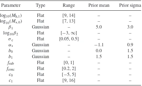
Table 2. Priors adopted in halo model fit.

Parameter Type Range Prior mean Prior sigma

log10(Mh,1) Flat [9, 14] – –

log10(M∗,0) Flat [7, 13] – –

β1 Gaussian – 5.0 3.0

log10β2 Flat [−3,∞] – –

σc Flat [0.05, 0.5] – –

αs Gaussian – −1.1 0.9

b0 Gaussian – 0.0 1.5

b1 Gaussian – 1.5 1.5

fsub Flat [0, 1] – –

fconc Flat [0.2, 2] – –

c0 Flat [−5, 5] – –

c1 Flat [9, 16] – –

the addition of a quadratic term in equation (18), in Appendix B. We find that our results are not significantly affected.

We assign a mass to the subhaloes in which the satellites re-side using the same relation that we use for the centrals (equation 16). For every stellar mass bin, we compute the average mass of the main haloes in which the satellite resides, and multiply this with a constant factor,fsub, a free parameter whose range is limited

to values between 0 and 1. In this way, we can crudely account for the stripping of the dark matter haloes of satellites. Given our limited knowledge of the distribution of dark matter in satellite galaxies, we assume that it is described by an NFW profile, which provide a decent description of the mass distribution of subhaloes in the Millennium simulation (Pastor Mira et al.2011). We use the same mass–concentration relation as for the centrals. The statistical power of our measurements is not sufficient to additionally fit for a truncation radius (see Sif´on et al.2015).

The above prescription provides us with the lensing signal from centrals and satellites, with separate contributions from their one-halo and two-one-halo terms. At small projected separations, the contri-bution of the baryonic component of the lenses themselves becomes relevant. We model this using a simple point mass approximation:

1h gal(R)≡

M∗

π R2, (19)

with M_∗the average stellar mass of the lens sample.

To summarize, the halo model employed in this paper has the following free parameters: (Mh,1, M∗,0, β1, β2, σc) and (αs,b0,b1)

to describe the halo occupation statistics of centrals and satellites.

fsubcontrols the subhalo masses of satellites, andfconc quantifies

the normalization of thec(M) relation. We use non-informative flat or Gaussian priors, as listed in Table2, except forβ1, because our

measurements do not extend far below the location of the kink in the stellar-to-halo mass relation. As a consequence, we are not able to provide tight constraints on the slope at the low-mass end. All priors were chosen to generously encapsulate previous literature results and they do not affect our results. In particular, in Appendix B we demonstrate that our results are insensitive to the choice of prior on β1. Note that for some samples, we had to adopt somewhat different

priors; we comment on this where applicable.

The parameter space is sampled with an affine invariant ensem-ble Markov Chain Monte Carlo (MCMC) sampler (Goodman & Weare2010). Specifically, we use the publicly available codeEMCEE

(Foreman-Mackey et al.2013). We runEMCEEwith four separate

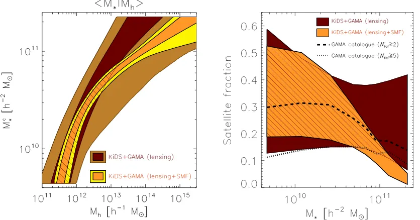
Figure 3. (Left) stellar-to-halo mass relation of central galaxies from KiDS+GAMA, determined from fitting the lensing signal only (dark/light brown indicating 1/2σmodel uncertainty regime) or by combining the lensing signal with the stellar mass function (orange/yellow indicating 1/2σmodel uncertainty regime). The contours are cut at the mean stellar mass of the first and last stellar mass bin used in the lensing analysis, to ensure we only show the regime where the data constrains it. (Right) the fraction of galaxies that are satellites as a function of stellar mass for all GAMA galaxies. The coloured contours show the 68 per cent confidence interval for the fits to the lensing signal only and to the combined fits, as indicated in the panel. The upper thick black dashed line shows a crude estimate of the satellite fraction based on the GAMA group catalogues (as detailed in Section 3.3), the lower thick dotted line shows a lower limit. Hatched areas show the overlap between the 1σlensing-only results and the combined analysis.

we estimate the parameter uncertainties; the fit parameters that we quote in the following correspond to the median of the marginalized posterior distributions, the errors correspond to the 68 per cent confidence intervals around the median. We assess the convergence of the chains with the Gelman–Rubin test (Gelman & Rubin1992) and ensure thatR≤1.015, withRthe ratio between the variance of a parameter in the single chains and the variance of that parameter in all chains combined. In addition, we compute the auto-correlation time (see e.g. Akeret et al.2013) for our main results and find that it is shorter than the length of the chains that is needed to reach 1 per cent precision on the mean of each fit parameter.

For some lens selections, we also run the halo model in an ‘in-formed’ setting. When we use the GAMA group catalogue to select and analyse only centrals or satellites, we only need the part of the halo model that describes their respective signals. Hence, when we only select centrals, we set the CSMF of satellites to zero. When we select satellites only, we model both the CSMF of the satellites and of the centrals of the haloes that host the satellites. We need the latter to model the miscentred one-halo term and the subhalo masses of the satellites.

3 S T E L L A R - T O - H A L O M A S S R E L AT I O N

We start with an analysis of the lensing measurements to examine the stellar-to-halo mass relation of central galaxies, as was done in several previous studies (e.g. Mandelbaum et al.2006; van Uitert et al.2011; Velander et al.2014). We fit the lensing signals of the eight lens samples simultaneously with the halo model. The best-fitting models from the lensing-only analysis can be compared to the data in Fig.2. The resulting reduced chi-squared,χ2

red, has a

value of 1.0 (with 70 degrees of freedom), so the models provide a satisfactory fit. In the left-hand panel of Fig.3 we show the

constraints on the stellar-to-halo mass relation. A broad range of relations describe the lensing signals equally well. Furthermore, the right-hand panel of Fig.3shows that the uncertainties on the fraction of galaxies that are satellites is also large.

van Uitert et al. (2011) pointed out that the uncertainties on the satellite fraction obtained from lensing only are large at the high stellar mass end, and, even worse, that a wrongly inferred satel-lite fraction can bias the halo mass as they are anti-correlated. The reason for this degeneracy is that lowering the halo mass reduces the model excess surface mass density profile, which can be partly compensated by increasing the satellite fraction, as satellites reside on average in more massive haloes than centrals of the same stellar mass, thereby boosting the model excess surface mass density pro-file at a few hundred kpc. This problem was partly mitigated in van Uitert et al. (2011) and Velander et al. (2014) by imposing priors on the satellite fractions, which is not ideal, as the results are sensitive to the priors used. As we employ a more flexible halo model here, this problem is exacerbated and a different solution is required.

In order to tighten the constraints on the satellite fraction and the stellar-to-halo mass relation, we either need to impose priors in the halo model, or include additional, complementary data sets. Since it is not obvious what priors to use, particularly since we aim to study how the stellar-to-halo mass relation depends on environment, we opt for the second approach. The most straightforward complemen-tary data set is the stellar mass function, which constrains the central and satellite CSMFs through equation (14). As a result, the number of satellites cannot be scaled arbitrarily up or down anymore, which helps to break this degeneracy.

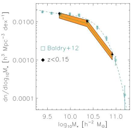
Figure 4. Stellar mass function determined using all GAMA galaxies at

z <0.15. Orange regions indicate the 68 per cent confidence interval from

the halo model fit to the lensing signal and the stellar mass function, linearly interpolated between the stellar mass bins. The solid green line indicates the best-fitting model. The stellar mass function from Baldry et al. (2012), determined using GAMA galaxies atz <0.06, is also shown.

9.39<log₁₀(M_∗/h−2M)<11.69 and include all galaxies from the G3_{Cv7 group catalogue withz <0.15. The choice of the number}

of bins is mainly driven by the low number of independent boot-strap realisations we can use to estimate the errors (discussed in Appendix A). We do not expect to lose much constraining power from the stellar mass function by measuring it in three bins only. Note that the mean lens redshift is somewhat higher than the redshift at which we determine the stellar mass function, but the evolution of the stellar mass function is very small over the redshift range considered in this work (see, e.g. Ilbert et al.2013) and hence can be safely ignored. The stellar mass function is shown in Fig. 4, together with the results from Baldry et al. (2012), who measured the stellar mass function for GAMA using galaxies atz <0.06. The measurements agree well.

We determine the error and the covariance matrix via bootstrap-ping, as detailed in Appendix A. We show there that (1) the boot-strap samples should contain a sufficiently large physical volume. If the sample volume is too small, the errors will be underestimated; (2) the major contribution to the error budget comes from cosmic variance. The contribution from Poisson noise is typically of or-der 10–20 per cent; (3) the stellar mass function measurements are highly correlated. Smith (2012) showed that this has a major impact on the confidence contours of model parameters fitted to the stellar mass function. Including the covariance is therefore essential, not only for studies that characterize the stellar mass/luminosity func-tion (for example as a funcfunc-tion of galaxy type), but also when it is used to constrain halo model fits.

To determine the cross-covariance between the shear measure-ments and the stellar mass function, we measured the shear of all GAMA galaxies with log10(M∗/h−2M)>9.39 andz <0.15 in

each KiDS pointing, and used the same GAMA galaxies to de-termine the stellar mass function. These measurements were used as input to our bootstrap analysis. The covariance matrix of the combined shear and stellar mass function measurements revealed that the cross-covariance between the two probes is negligible and

can be safely ignored. The covariance between the lensing mea-surements and the stellar mass function for smaller subsamples of GAMA galaxies is expected to be even smaller because of larger measurement noise. Therefore, we do not restrict ourselves to the overlapping area with KiDS, but use the entire 180 deg2_{of GAMA}

area to determine the stellar mass function to improve our statistics. We fit the lensing signal of all bins and the stellar mass function simultaneously with the halo model. The best-fitting models are shown in Figs2and4, together with the 1σ model uncertainties. The reducedχ2 _{of the best-fitting model is 80/(83− 10)= 1.1}

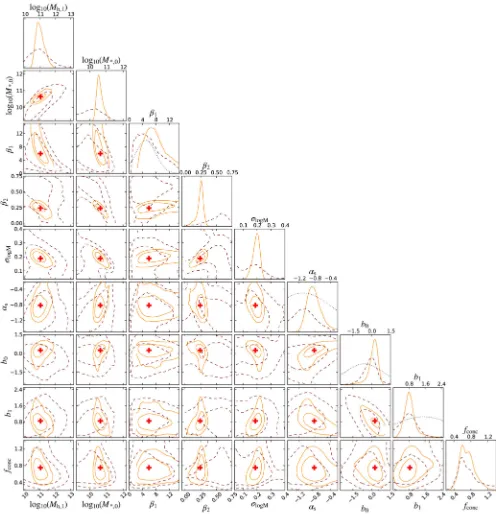
(eight mass bins times 10 angular bins for the lensing signal, plus three mass bins for the stellar mass function), so the halo model provides an appropriate fit. The lensing signal of the best-fitting model is virtually indistinguishable from the best-fitting model of the lensing-only fit. The stellar-to-halo mass relation, however, is better constrained, as is shown in Fig. 3. The relation is flatter towards the high-mass end, as a result of a better constrained satellite fraction that decreases with stellar mass (discussed in Section 3.3). The constraints on the parameters are listed in Table 3. The marginalized posteriors of the pairs of parameters are shown in Fig.5. This figure illustrates that the main degeneracies in the halo model occur between the parameters that describe the stellar-to-halo mass relation, and between the parameters that describe the CSMF of the satellites. These degeneracies are expected, given the functional forms that we adopted (see equations 16, 17, 18). For example, a larger value forMh,1would decrease the amplitude of the

stellar-to-halo mass relation, which could be partly compensated by increasingM_∗,0; hence these parameters are correlated. Similarly,

increasingb0would lead to a higher normalization ofs(M∗|M),

which could be partly compensated by decreasingb1, hence these

two parameters are anti-correlated. Furthermore, by comparing the marginalized posteriors to the priors, we observe that all parameters but one,β1, are constrained by the data. We have verified that

varying the prior onβ1 does not impact our results. Comparing

the posteriors of the combined fit to the analysis where we only fit the lensing signal reveals that the stellar mass function helps by constraining several parameters; those that describe the stellar-to-halo mass relation and those that describe the satellite CSMF.

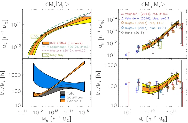
In Fig.6, we present the stellar-to-halo mass relation of central galaxies and the ratio of halo mass to stellar mass. The relation con-sists of two parts. This is not simply a consequence of adopting a double power law for this relation in the halo model, since the fit has the freedom to put the pivot mass below the minimum mass scale we probe, which would effectively result in fitting a single power law. ForM∗<5×1010_h−2_M

, the stellar-to-halo mass relation is fairly steep and the stellar mass increases with halo mass as a power law ofMhwith an exponent∼7. At higher stellar masses, the

relation flattens to∼M0.25

h . The ratio of the dark matter to stellar

mass has a minimum at a halo mass of 8×1011_h−1_M

, where Mc

∗=(1.45±0.32)×1010h−2M and the halo mass to stellar

mass ratio has a value ofMh/M∗=56+16−10[h]. The uncertainty on

this ratio reflects the errors on our measurements and does not ac-count for the uncertainty of the stellar mass estimates themselves, which are typically considerably smaller than the bin sizes we adopted and hence should not affect the results much. The loca-tion of the minimum is important for galaxy formaloca-tion models, as it shows that the accumulation of stellar mass in galaxies is most efficient at this halo mass.

In the lower left-hand panel of Fig. 6, we also show the inte-grated stellar mass content of satellite galaxies divided by halo mass. In haloes with masses2×1013_h−1_M

log10(Mh,1) log10(M∗,0) β1 β2 σc b0 b1 αs fsub fconc c0 c1

(1) (2) (3) (4) (5) (6) (7) (8) (9) (10) (11) (12)

All 10.97+0₋₀._.34₂₅ 10.58+0₋₀._.22₁₅ 7.5₋₂+3._.8₇ 0.25₋₀+0_..04₀₆ 0.20+0₋₀._.02₀₃ 0.18+0₋₀._.28₃₉ 0.83+0₋₀._.27₂₃ −0.83₋₀+0._.1622 0.59+0_−0..₄₀31 0.70+0₋₀._.19₁₅ – – Cen 12.06+₋0_0..₈₀72 11.16+₋0₀._.40₆₂ 5.4+₋5₃._.3₄ 0.15+₋0₀._.31₁₄ 0.14+₋0₀._.08₀₅ – – – – 0.77+₋0₀._.1827 2.05+₋1_0..₈₂88 13.00+₋0₀._.28₁₃

Sat 0.12₋₀+0_..19₂₆ 0.71+₋₀0._.12₁₃ −1.03+₋₀0._.07₀₈ 0.25₋₀+0_..09₀₈ 0.94₋₀+0._.18₁₆ Sat 11.70+0₋₀._.70₈₄ 11.22₋₀+0._.12₂₂ 4.5+4₋₂._.96 0.05+0_−0..07₀₄ 0.12+0_−0..12₀₅ −0.14₋₀+0._.2863 1.03+0₋₀._.14₃₃ −1.00+0₋₀._.10₁₂ 0.40+0₋₀._.2143 1.05+0₋₀._.25₁₈ 1.03₋₁+2_..89₀₁ 12.09+2₋₁._.71₈₆

5×1014_h−1_M

∼94 per cent of the stellar mass is in satellite galaxies. Note that another considerable fraction of stellar mass is contained in the diffuse intra-cluster light (up to several tens of per-cents, see e.g. Lin & Mohr2004) which we have not accounted for here. The recently discovered ultra-diffuse galaxies (e.g. Abraham & van Dokkum2014; van der Burg, Muzzin & Hoekstra 2016) form yet another source of unaccounted for stellar mass, but how much they contribute to the total stellar mass budget is currently uncertain.

The normalization of the mass–concentration relation is fairly low,fconc=0.70+₋00..1915. A normalization lower than unity was

antic-ipated as we did not account for miscentring of centrals in the halo model. Miscentring distributes small-scale lensing power to larger scales, an effect similar to lowering the concentration. In our fits, it merely acts as a nuisance parameter, and should not be interpreted as conflicting with numerical simulations. In future work, we will include miscentering of centrals in the modelling, which should enable us to derive robust and physically meaningful constraints onfconc. The subhalo mass of satellites is not constrained by our

measurements, which is why we do not show it in Fig.5. This is not surprising, given that most of our lenses are centrals, and that the lensing signal is fairly noisy at small projected distances from the lens.

3.1 Sensitivity tests on stellar-to-halo mass relation

We have performed a number of tests to examine the robustness of our results. For computational reasons, we limited the number of model evaluations to 750 000 (instead of 2100 000), divided over two chains. We adopted a maximum value ofR= 1.05 in the Gelman–Rubin convergence test to ensure that results are suffi-ciently robust to assess potential differences.

First, we test if incompleteness in our lens sample can bias the stellar-to-halo mass relation. As GAMA is a flux-limited survey, our lens samples miss the faint galaxies at a given stellar mass. If these galaxies have systematically different halo masses, our stellar-to-halo mass relation may be biased. To check whether this is the case, we selected a (nearly) volume-limited lens sample using the methodology of Lange et al. (2015). This method consists of deter-mining a limiting redshift for galaxies in a narrow stellar mass bin, zlim, which is defined as the redshift for which at least 90 per cent of

the galaxies in that sample havezlim< zmax, withzmaxthe maximum

redshift at which a galaxy can be observed given its rest-frame SED and given the survey magnitude limit.zlimis determined iteratively

using only galaxies withz < zlim. We removed all galaxies with

red-shifts larger thanzlim(∼60 per cent of the galaxies in the first stellar

mass bin, fewer for the higher mass bins) and repeated the lensing

measurements. The resulting measurements are a bit noisier, but do not differ systematically. We fit our halo model to this lensing signal and the stellar mass function. The resulting stellar-to-halo mass relation becomes broader by up to 20 per cent at the low-mass end, but is fully consistent with the result shown in Fig.6. Hence we conclude that incompleteness of the lens sample is unlikely to significantly bias our results.

We have also tested the impact of various assumptions in the set up of the halo model. We give details of these tests in Appendix B. None of the modifications led to significant differences in the stellar-to-halo mass relation, which shows that our results are insensitive to the particular assumptions in the halo model.

3.2 Literature comparison

We limit the literature comparison to some of the most recent results, referring the reader to extensive comparisons between older works in Leauthaud et al. (2012); Coupon et al. (2015); Zu & Mandelbaum (2015). Our main goal is to see whether our results are in general agreement. In-depth comparisons between results are generally dif-ficult, due to differences in the analysis (e.g. the definition of mass, choices in the modelling) as well as in the data (e.g. the computation of stellar masses – note, however, that the stellar masses used in the literature stellar-to-halo mass relations we compare to are all based on a Chabrier (2003) IMF, as are ours).

Leauthaud et al. (2012) measured the stellar-to-halo mass rela-tion of central galaxies by simultaneously fitting the galaxy–galaxy lensing signal, the clustering signal and the stellar mass function of galaxies in COSMOS. The depth of this survey allowed them to measure this relation up toz=1. In Fig.6, we show their relation for their low-redshift sample at 0.22< z <0.48, which is closest to our redshift range. The relations agree reasonably well. We infer a slightly larger halo mass at a given stellar mass, most noticeably at the high-mass end. TheirMh/M∗ratio reaches a minimum at a

halo mass of 8.6×1011_h−1_M

with a value ofMh/M∗=38 [h],

Figure 5. Posteriors of pairs of parameters, marginalized over all other parameters. Dimensions are the same as in Table3. Solid orange contours indicate the 1/2σconfidence intervals of the lensing+SMF fit, while the brown dashed contours indicate the 1/2σconfidence intervals of the lensing-only fit. Red crosses indicate the best-fitting solution of the combined fit. The panels on the diagonal show the marginalized posterior of the individual fit parameters, together with the priors (blue dotted lines). Including the SMF in the fit mainly helps to constrain the stellar-to-halo mass relation parameters (equation 16) andαs. The degeneracies between the stellar-to-halo mass relation parameters and those that describe the satellite CSMF (equation 17, 18), follow from the functional form we adopted.

typically of this order (see e.g. Mobasher et al.2015), which implies that the accuracy of the stellar-to-halo mass relation is already lim-ited by systematic uncertainties in the stellar mass estimates.

Next, we compare our results to Moster et al. (2013), who applied an abundance matching technique to the Millennium simulation (Springel 2005). The stellar mass functions were adopted from various observational studies, but were all converted to agree with a

Chabrier (2003) IMF. We use the fitting functions provided in that work to compute the stellar-to-halo mass relation atz=0.25, close to the mean redshift of our full sample. We find good agreement between the results as shown in Fig. 6. The minimum of their Mh/M∗ ratio is located at 7 ×1011h−1M, close to our

best-fitting result of 8×1011_h−1_M

Figure 6. Stellar-to-halo mass relation of central galaxies for KiDS+GAMA. Orange (yellow) regions indicate the 68 per cent (95 per cent) confidence intervals for the centrals, blue regions the 68 per cent confidence intervals for the satellites, and grey (solid and hatched) regions are the 68 per cent confidence intervals for the total sample. Our results can be compared to constraints from Leauthaud et al. (2012), Moster et al. (2013), Wojtak & Mamon (2013), Velander et al. (2014), Han et al. (2015), and from the Milky Way. Note that the left-hand panels show the stellar mass at a given halo mass, M∗|Mh, while the

right-hand panels show the halo mass at a given stellar mass, Mh|M∗.

We compare our measurements to the results of Han et al. (2015) in the right-hand panel of Fig.6. Han et al. (2015) measured halo masses for the same GAMA sample, but using sources from the SDSS. Halo masses were estimated for a volume-limited lens sam-ple using a maximum likelihood technique. In contrast to our work, their measurements show the average halo mass for a given stellar mass, which is not the same due to the intrinsic scatter (see e.g. fig. 7 of Tinker et al.2013). Hence we converted our results using Bayes theorem (see e.g. Coupon et al.2015) to enable a comparison. We find excellent agreement between the results.

Wojtak & Mamon (2013) present halo mass estimates for galax-ies in stellar mass bins obtained from the kinematics of satellite galaxies around isolated galaxies in the SDSS. Halo masses were defined with respect toρcritinstead of the mean density, which are

typically 30–40 per cent smaller. To account for this, we multiplied their masses with a factor 1.3. We find good agreement at stellar massesM_∗<8×1010_h−2_M

, but at higher stellar masses their halo masses are somewhat lower than ours. A potential reason is that their sample only consists of isolated galaxies, which may have sys-tematically lower halo masses. Also note that they remark in their work that their halo masses are∼0.2 dex lower at the high-mass end than what is typically reported in the literature.

Finally, we compare our results to the galaxy–galaxy lensing results from Velander et al. (2014), who measured the lensing signal around red and blue galaxies at 0.2< z <0.4 in CFHTLenS over a large range in stellar mass. Masses were defined with respect toρcrit, which we multiplied with a factor 1.3 to convert them to

our definition. The agreement is fair; we find a good match at low stellar masses, but forM_∗>5×1010_h−2_M

, our halo masses are somewhat larger. What may be contributing to this difference, is that Velander et al. (2014) inferred a relatively high satellite fraction for red galaxies at the high stellar mass end (reaching as high as their upper limit of 0.2), which may have pushed their average halo mass

down. Also, as for Leauthaud et al. (2012), stellar masses were determined using photometric redshifts, which may have induced a small Eddington bias. If we decrease their mean stellar masses by 0.1 dex, their measurements fully overlap with ours.

Summarizing the above, we conclude that although we find small differences between our stellar-to-halo mass relation and those from the literature, the agreement is fair in general.

3.2.1 Milky Way comparison

The number of satellite galaxies depends on halo mass, and obser-vations of the Milky Way suggest that it may have fewer satellites than expected given its stellar mass (e.g. Klypin et al.1999; Moore et al.1999). To resolve this so-called ‘missing satellite problem’ various studies have shown that the tension is eased for lower halo masses of the Milky Way (e.g. Wang et al.2012; Vera-Ciro et al. 2013). This raises the question whether or not the location of the Milky Way is special in the stellar mass to halo mass plane, i.e. whether its halo mass is peculiarly low given its stellar mass.

Total stellar mass estimates for the Milky Way are typically of order (6 ±1)×1010_M

(McMillan 2011; Licquia & Newman 2015). Halo mass estimates have a considerably larger scatter, with

M200 estimates ranging (0.5–2) ×1012M (see fig. 1 of Wang

et al.2015). We adjust these local measurements assumingh=0.7 and show the results in Fig.6. Our stellar-to-halo mass relation predicts a mean stellar mass of 1.8×1010_h−2_M

at a halo mass of 1×1012_h−1_M

. The Milky Way lies just at the edge of our 1σ contours. However, our confidence intervals only correspond to the uncertainties on the mean relation, and when comparing individual objects, one should take the intrinsic scatter between stellar and halo mass, which is∼0.2 dex, into account. Hence the lower limit on the stellar mass of the Milky Way (5×1010_M

away in terms of intrinsic scatter atMh=1012h−1M. Although

the Milky Way appears to have a relatively high stellar mass given its halo mass, it is not particularly anomalous.

3.3 Satellite fraction

Our sample consists of a mixture of central and satellite galaxies. In the halo model we fit for the contribution of both, which enables us to determine the satellite fraction using equation (13). The results are shown in Fig.3. The satellite fraction decreases with stellar mass from∼0.3 at 5×109_h−2_M

to∼0.05 at 2×1011_h−2_M

. Particularly at the high-mass end, it is well constrained. As for the stellar-to-halo mass relation, including the constraints from the stellar mass function has a significant impact and considerably de-creases the model uncertainty. The satellite fraction does not sen-sitively depend on assumptions in the halo model, as discussed in Appendix B.

We compare our satellite fractions to those based on the GAMA group catalogue. For every stellar mass range, we count all galaxies listed as satellite (not restricted to groups withNfof≥5), and divide

that by the total number of galaxies in that range. We only include GAMA galaxies atz <0.3 here, to reduce the impact of incomplete-ness. The resulting satellite fractions do not sensitively depend on the specific value of the redshift cut. The ratio is shown as the upper dashed line in Fig.3. It provides an estimate of the true satellite fraction, but a crude one as the group membership identification in GAMA becomes less robust towards groups with fewer members (Robotham et al.2011) and we do not apply a cut onNfof. Hence

a fraction of the galaxies that are labelled as satellites may in fact be centrals. In addition, some satellites may not be identified and as such be excluded from the group catalogue. We derive a more robust lower limit on the satellite fraction by only counting the satellites in ‘rich’ groups (Nfof≥5) and dividing that by the total number of

galaxies in that stellar mass range. This is indicated by the lower dotted line in Fig.3. The satellite fraction we obtain from the halo model should be larger than this, which we find to be the case at M∗<1011h−2M. For higher stellar masses, our constraints on

the satellite fraction fall below the lower limit from the GAMA catalogue. Although not very significant, it suggests that a fraction of satellites at the high stellar mass end are actually centrals, or that one or more assumptions in our halo model are inaccurate. Either way, it shows that the combination of galaxy–galaxy lensing with the stellar mass function has the potential to become a valuable tool to infer the robustness of group catalogues. We expect that including the clustering of galaxies in the fit will further tighten the constraints on the satellite fraction (see e.g. Cacciato et al.2009).

4 E N V I R O N M E N TA L D E P E N D E N C E

Galaxies in groups are subject to processes such as quenching, stripping and merging. One of the observable consequences is that star formation is suppressed and galaxies turn red (see e.g. Boselli & Gavazzi2006). The cumulative impact of these processes is likely to affect the baryonic and dark matter content of centrals and satellites in different ways. An infalling (satellite) galaxy, for example, is expected to lose relatively more dark matter than stars, as the latter mainly reside in the central part of the halo where the potential well is deep (e.g. Wetzel et al.2014). This increases the group halo mass, but should not affect the stellar mass of the central much. If, on the other hand, an already accumulated satellite that has been stripped off its dark matter merges with the central galaxy, the stellar mass of the central increases, but not the halo mass. By comparing the

stellar-to-halo mass relation for centrals in ‘rich’ groups to the one of the full sample, we can study the relative importance of such environmental effects.

4.1 Centrals in rich groups

We first select the central galaxies in ‘rich’ groups (with a multi-plicityNfof≥5) and measure their lensing signal and stellar mass

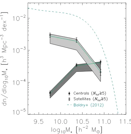
function using the same binning as before. We exclude groups with fewer than five members because comparisons with mock data have shown that those are affected more by interlopers (Robotham et al. 2011), which makes an interpretation of the results harder. The galaxy–galaxy lensing signal is shown in Fig. 7and the stellar mass function in Fig.8. We measure the stellar mass function using groups atz <0.15 to ensure the sample is volume-limited.

To fit the halo model to the data, we have to account for one additional complication. For certain sub-samples of galaxies, not all haloes of massMcontain a central galaxy, while the halo model assumes that all of them do (the integral of equation 15 over stellar mass is unity). We account for this by introducing a ‘halo mass incompleteness’ factor, a generic function that varies between 0 and 1, which we multiply with the CSMF of the central galaxies:

c(M∗|Mh)=c(M∗|Mh)×erf(c0[log10(Mh)−c1]), (20)

withc0andc1two incompleteness parameters that we fit for;c1

de-termines where we the transition to incompleteness occurs, andc0

determines how smooth or abrupt the transition is. This incomplete-ness factor is only suitable for selections of lenses whose abundance as a function of stellar mass increases/decreases monotonically with respect to the full sample, as is the case here. A similar approach was taken in Tinker et al. (2013) in order to simultaneously mea-sure the stellar-to-halo mass relation of quiescent and star-forming galaxies (see their Section 3.2).

To fit the halo model, we need to apply priors on the incomplete-ness parameters (c0,c1), as the large covariance of the three stellar

mass function bins results in a peculiar likelihood surface. For a large range of (c0,c1) values, theχ2of the stellar mass function

is high but practically constant. When the MCMC chains start far from the minimum, they can get stuck in thisχ2_{plateau. To avoid}

having to run very long chains to ensure all walkers find their way to the minimum, we adopt flat priors and restrictc0to [−5, 5] and

c1to [9, 14] which generously brackets the best fit for any chain

we run and hence should not affect the results. Note that we adopt a range of [9, 16] forc1for all other runs, see Table2. We start

the chains close to the best-fitting location, as determined from a previous run, to avoid that many walkers start in thisχ2_{plateau and}

never reach the minimum. Even with these precautions, a fraction (10 per cent) of the chains remain stuck.3_{Since those models have}

a similar (large)χ2 _{contribution from the stellar mass function,}

we can easily identify them and remove them before we analyse the chain. Fig.8shows that the model uncertainty of the stellar mass function is somewhat skewed with respect to the data and the best-fitting halo model. The reason is that some of the walkers are close to theχ2_{plateau and still in the process of evolving towards}

the minimum. We have checked that including these problematic walkers does not affect our results.

3_{We also implemented a Metropolis–Hastings sampler with a proposal}

Figure 7. Excess surface mass density profile of GAMA galaxies measured as a function of projected separation to the lens, selected in various stellar mass bins as indicated at the top of each column, that are centrals (top row) and satellites (bottom row) of ‘rich’ (Nfof≥5) groups. The bin ranges correspond to the

log10of the stellar mass and are in units log10(h−2M). Open symbols and the dashed lines indicate the absolute value of the negative data points and their

errors. The green solid line indicates the best-fitting halo model, the grey contours indicate the 68 per cent model uncertainty.

Figure 8. Stellar mass functions for GAMA galaxies atz <0.15 that are centrals and satellites in ‘rich’ groups, for a comoving volume. Errors have been determined by bootstrap and include the contributions from Poisson noise and cosmic variance. The green solid line indicates the best-fitting halo model, the grey regions indicate the 68 per cent model uncertainty, linearly interpolated between the stellar mass bins. We also show the analytical fit to the SMF from Baldry et al. (2012) for all galaxies for reference. The model uncertainties are somewhat skewed with respect to the data and the best-fitting model, which is caused by sampling issues, as discussed in the text.

The best-fitting model has a reducedχ2_{of 98/(83−8)=1.3.}

Fig.7shows that the lensing signal of the lowest stellar mass bin is not well fit. A possible reason is that the lowest stellar mass sam-ples are contaminated with satellite galaxies, for which we provide evidence in Section 4.3. Note that the lensing signal of these bins are very noisy and that a potential bias of the stellar-to-halo mass

relation at the low-mass end resulting from this contamination is unlikely to be significant.

The constraints on the fit parameters are tabulated in Table3. The stellar-to-halo mass relation is shown in Fig.9. The 68 per cent confidence interval is broader than the one of the full sample due to the noisier lensing measurements at the low stellar mass end. None the less, it shows that the stellar-to-halo mass relation of centrals in ‘rich’ groups is consistent with the relation for the full sample, suggesting that this relation does not sensitively depend on local density. Note that centrals in ‘rich’ groups form∼15 per cent of the total lens sample for the two highest stellar mass bins, so the average lensing signals of centrals in those bins are somewhat correlated to the lensing signals of the corresponding bins of the full sample (and consequently, the stellar-to-halo mass relations will be correlated as well at the high-mass end).

We also inferred the stellar-to-halo mass relation from the lens-ing signal only. The resultlens-ing minimum χ2 _{is 97 with 72}

de-grees of freedom, hence a similar reducedχ2_{as for the combined}

fit. The stellar-to-halo mass relation is consistent, but less well constrained than the combined fit, particularly at stellar masses >2×1010_h−2_M

, where the upper limit in halo masses is shifted to larger values, already extending to 1015_h−1_M

at stellar masses of 8×1010_h−2_M

.

Our result appears somewhat at odds with Tonnesen & Cen (2015), who studied environmental variations of the stellar-to-halo mass ratio using a large suite of cosmological hydrodynamical sim-ulations. Environments were classified according to the mean den-sity on 20 Mpc scales, stellar mass were computed by adding the mass of all star particles that belonged to a galaxy. They reported a significantly larger stellar-to-halo mass ratio for galaxies in large-scale overdensities, compared to those in large-large-scale underdensities. Their most massive halo mass bin extends to 1013_h−1_M