Aeroelastic flutter as a multiparameter eigenvalue problem

(1)

Aeroelastic flutter as a multiparameter

eigenvalue problem

by

Arion Pons

Submitted in partial fulfilment of the requirements

for the degree of

Master of Engineering

in the Department of Mechanical Engineering

at the University of Canterbury.

(2)

Page ii TABLE OF CONTENTS

Table of Contents ii

Acknowledgements v

Abstract vi

Nomenclature vii

Preface viii

Chapter 1 – Initial manoeuvres 1

1.1 Introduction and scope 1

1.2 Central thesis 6

1.3 Extensions 8

1.4 References 9

Chapter 2 – Index of systems 14

2.1 Introduction 14

2.2 An introductory model 15

2.3 A section model with unsteady aerodynamics 18

2.3.1 Formulation in and 18

2.3.2 Other formulations 22

2.3.3 Quasisteady aerodynamics 23

2.3.4 Quasisteady aerodynamics with no structural damping 23

2.3.5 Approximations to Theodorsen’s function 23

2.3.6 Parameter values 27

2.4 References 27

Chapter 3 – Visualisation methods 28

3.1 The purpose of visualisation method 28

3.2 Modal damping and root locus 28

3.3 Contour plot 35

3.4 Numerical experiments 38

3.4.1 Simple section model 38

3.4.2 Undamped section model with quasisteady aerodynamics 40 3.4.3 Section model with quasisteady aerodynamics 42 3.4.4 Section model with Theodorsen aerodynamics 49

3.5 Concluding remarks 54

3.6 References 56

Chapter 4 – Structured systems 58

4.1 Introduction 58

4.2 Linear problems 58

4.2.1 Motivation 58

4.2.2 The Kronecker product 59

4.2.3 The operator determinant method for two-parameter systems 59

(3)

Page iii

4.2.5 Computational complexity 63

4.2.6 Numerical experiments 63

4.3 Quadratic problems 67

4.3.1 Motivation 67

4.3.2 Linearisation 68

4.3.3 Quasi-linearisation 70

4.3.4 The general operator determinant method 71

4.3.5 Computing operator determinants 74

4.4 Problems of higher order 80

4.4.1 Motivation 80

4.4.2 The Jones approximation 80

4.4.3 The fractional-order approximation 81

4.4.4 Optimality of linearisations 83

4.5 Other linear solvers 93

4.5.1 Sylvester-Arnoldi 94

4.5.2 Subspace methods 94

4.7 References 96

Chapter 5 – Semi-structured systems 100

5.1 Introduction 100

5.2 Picard iteration 101

5.2.1 Formulation 101

5.2.2 Specific algorithms 107

5.2.3 A single-parameter iterative method 109

5.3 Newton iteration 115

5.3.2Numerical experiments 118

5.4 Higher-order methods 121

5.6 References 123

Chapter 6 – Unstructured systems 124

6.2 The method of successive linear problems (SLP) 126

6.2.2 Specific algorithms 129

6.3 The iterated contour plot / Newton’s method 136

(4)

Page iv

6.4 Higher-order methods 144

6.4.1 Motivation 144

6.4.2 A second-order iterated contour plot method 144

6.4.4 Retrospective review 150

6.5 Other Newton-type methods 151

6.5.1 Iteration based on minimum singular value 152

6.5.2 Full eigenvalue / eigenvector iteration 153

6.5.3 Tensor Rayleigh quotient iteration (TRQI) 155

6.6 Singular vector iteration (SVI) 156

6.6.1 Initial manoeuvres 156

6.6.2 The singular value decomposition 156

6.6.3 The Rayleigh quotient 157

6.6.4 Implementation and variants 160

6.7 Restriction 167

6.8 Deflation 172

6.8.1 Theory 172

6.9 Assessment and conclusion 181

6.9.1 General assessment 181

6.9.2 Conclusions 185

6.10 References 185

Chapter 7 – Concluding remarks 188

7.2 Assessment of methods 188

7.2.1 Solvers for structured problems 188

7.2.2 Solvers for semi-structured systems 192

7.2.3 Solvers for unstructured problems 193

7.3 Constrainedness 195

7.4 Further extensions 196

7.5 Summary of future research opportunities 197

7.6 Final conclusion 198

(5)

Page v ACKNOWLEDGEMENTS

(6)

Page vi ABSTRACT

In this thesis we explore the relationship between aeroelastic flutter and multiparameter spectral theory. We first introduce the basic concept of the relationship between these two fields in abstract terms. Then we expand on this initial concept, using it to devise visualisation methods and a wide variety of solvers for flutter problems. We assess these solvers, applying them to real-life aeroelastic systems and measuring their performance. We then discuss and devise methods for improving these solvers. All our conclusions are supported by a variety of evidence from numerical experiments. Finally, we assess all of our methods, providing recommendations as to their use and future development.

(7)

Page vii NOMENCLATURE

imaginary unit

( ) real part of ( ) imaginary part of

matrix transpose of Hermitian transpose of

̇ time derivative of derivative of with respect to

Kronecker product | evaluation of at condition [ ] vertical concatenation of and [ ] horizontal concatenation of and

(8)

Page viii PREFACE

It is important that you read this preface. This thesis presents a synthesis of two areas of study which have not had any previous contact, and it is unlikely that the reader will have expertise in both of these areas. These areas are aeroelasticity and multiparameter spectral theory. This thesis has been written with aeroelasticians (i.e. engineers) in mind, and it concerned primarily with applying the tools available in multiparameter spectral theory to aeroelastic problems – as opposed to making any theoretical developments in multiparameter spectral theory per se. We will, in fact, often advance beyond what has currently been done in the theoretical literature on this subject (especially as regards our algorithms for nonlinear multiparameter eigenvalue problems). However, we would like to note up-front that readers with expertise in abstract mathematics will be unsatisfied by the standard of proof employed in this work. We will not attempt to prove results (e.g. convergence of iterative methods) in any other way than the application to a practical problem.

The structure of this thesis is relatively simple. Chapter 1 introduces the basic relationship between aeroelasticity and multiparameter spectral theory, upon which we will build everything else in the thesis. Chapter 2 introduces the physical aeroelastic systems that we will be working with. Chapters 3-6 are then go over a variety of difference system classes, and their respective solution methods. Each of these chapters is relatively distinct and may be read without much reference to the others. For this reason we have included a bibliography at the end of each chapter, in the place of one large bibliography at the very end. Chapter 7 presents a final conclusion and assessment of the previous six chapters, as well as a discussion on some further interesting phenomena and unsolved problems. Aeroelasticians or other engineers wanting to implement the methods presented in this thesis may find it easiest to locate the system of interested in the systems index (Chapter 2), and then

(9)

semis-Page ix

(10)

Chapter 1 – page 1

Chapter 1 Initial manoeuvres

1.1 INTRODUCTION AND SCOPE

Aeroelasticity is the field of study concerned with the interaction of an elastic structure in an airstream. As such, aeroelasticity can be seen as a subfield of the more general study of fluid-structure interaction (FSI), being concerned largely with the case when the working fluid is air. Alternately but equivalently, one might also see the field of aeroelasticity as the synthesis of the two fields of aerodynamics and structural dynamics – and this is indeed the historical origin of the field [1]. Aeroelasticity is thus of great relevance to the aeronautics industry: Hodges [2] notes that “the solution of many aeroelastic problems is a basic requirement for achieving an operationally reliable and structurally optimal [aerospace] system”. However, its applications in other areas – in particular, turbomachines and wind turbines – should not be overlooked.

One of the prime concerns in modern aeroelasticity is how to predict and control aeroelastic instability. An instability, in this context, may be defined as an event during which the structure in question becomes self-exiting. When this occurs dynamically (as an oscillatory instability) it is termed flutter, and when it occurs statically (as a non-oscillatory instability) it is termed divergence [3]. Divergence may be seen as a subsidiary form of flutter, and in this work we will use the term flutter to denote either instability. The term dynamic flutter will be used to denote flutter that is specifically oscillatory. In aeronautical systems, a number of different classes of flutter events may be observed. Some of the more important classes are [2–5]:

Classical flutter – a lifting surface at normal angle-of attack is exposed to subsonic flow.

Stall flutter – a lifting surface at high (stalling) angle-of-attack is exposed to subsonic flow.

(11)

Panel flutter – a non-lifting surface is exposed to flow.

Of course, for each of these classes there exist a large number of different mathematical models, for modelling different situations with different levels of accuracy. One easy distinction to make is between models based on linear and nonlinear systems1. In a linear aeroelastic system, the onset of flutter or divergence can be formulated in the well-known stability criterion:

( ) for stability (1.1.1)

where are the time-eigenvalues of the system according to the Fourier transform

( ) ̅ ( ) for the system coordinate . These eigenvalues are often nondimensionalised with respect to airspeed, but this is not relevant at this stage. In graphical terms, Eq. 1.1.1 means that eigenvalues in the upper half-plane of an Argand diagram are stable, and those in the lower half-plane are unstable2. Flutter occurs when the system parameters (airspeed, air density, etc.) are such that the system is on the point of crossing from stability into instability or vice-versa: that is, where ( ) . A given system may have many flutter points: each point is defined by a modal frequency and an airspeed value, with the air density and other parameters typically being fixed. Flutter points are always ordered by increasing airspeed: the first flutter point is the flutter point that occurs at the lowest (positive) airspeed value, etc. Dynamic flutter and divergence points are ordered separately, and those that occur at negative airspeed or frequency are irrelevant. Typically only the first flutter point and first divergence point are of industrial relevance. In an aircraft, the first aeroelastic instability alone will define the flight envelope of the aircraft – both flutter and divergence will typically result in catastrophic failure and the destruction of the flight vehicle [2].

In nonlinear systems, aeroelastic instabilities can be described by a number of nonlinear phenomena, including Hopf bifurcations and limit cycle oscillations [6,7]. The range of nonlinear models used in aeroelasticity is vast – ranging from analytical section models with

1

Please note the difference between a nonlinear eigenvalue problem and a nonlinear system.

2

(12)

simple nonlinearities, to fully-coupled FEA/CFD simulations. However, one should not suppose that the introduction of nonlinear models in aeroelasticity has made linear models obsolete, in industry or research: significant effort is still going into devising better methods for linear flutter point prediction. With the growing emphasis on optimisation of aircraft structures [8] and active aeroelastic control [9], low computation time for aeroelastic problems is imperative. Many computational models for flutter are based on linear theories – even for such turbulent systems as bridge decks under wind loading [10–13]. Most industrial aeronautical flutter solvers, such as MSC Nastran3 or ZAERO4, use linear potential-flow aerodynamics and solve their aeroelastic systems via frequency domain solvers [14,15]. Faster algorithms for such systems would have benefit to a wide range of industry. In recent years there has also been a proliferation of analytical models for novel aerodynamic / aeroelastic systems. These include models for camber-flutter in conformable wings [16,17], more accurate analytical flow models for helicopter blades [18–20], and a variety of biomechanical aeroelastic models involving fish [21], birds [22] and insects [23].

Our work will be concerned with linear aeroelastic systems, but even in this context it should be noted that Eq. 1.1 is not the only stability criterion that can be used to characterise aeroelastic flutter. Different ones can be devised, and even for a given criterion there may be a number of ways of devising and solving the associated system. This leads us into the study of aeroelastic methods, and it is worthwhile spending some time elaborating on these. There are four established methods in modern aeroelastic analysis: the p-method, classical flutter analysis, the k-method (or U-g method, or V-g method) and the p-k method [2]. The p-method is the most fundamental, and its use traces back to the earliest flutter analyses performed by British aerodynamicists after the First World War [24,25]. For this reason it is often referred to as the ‘British method’ in older literature [26]. The p-method simply involves solving the aeroelastic system for (or usually an equivalent nondimensional parameter ) over a range of airspeed values, and interpolating or otherwise estimating the points where Eq. 1.1 holds. If used with accurate aerodynamic and structural models, it can predict both the flutter points of the aeroelastic system and its modal characteristic at any airspeed. Its main disadvantage is that is requires an

3_{‘NASTRAN’ is a registered trademark of the National Aeronautics and Space Administration.} 4

(13)

aerodynamic model that is valid for the case when ( ) , and this is not always available [2]. This spurred the development of classical flutter analysis. This method involves deriving aeroelastic models based on the presumption that the system is at its flutter points ( ( ) ), and then solving these models (usually by a fixed-point iteration) for the conditions at which this is in fact true. One only has to have an aerodynamic model that is valid at the flutter point; such models are much easier to derive or obtain experimentally. Classical flutter analysis produces the same estimates of the flutter point locations as the p-method (for the same aeroelastic model, and assuming perfect convergence of the iterative method). However, it gives no information on the behaviour of the system away from its flutter points.

(14)

As can be seen, the difference between these methods is partly a matter of how the solution is solved mathematically, and how the real physical system is transferred into a mathematical model in the first place. In recent years there has been a proliferation of new aeroelastic methods. There has been an interest in the application of concepts from robust control theory; in particular, the linear fractional transformation and the structured singular value ( ). This yielded a series of methods based on dynamic pressure perturbation, including the -method by Lind and Brenner [28,29], the -k method by Borglund [30–33], the - method by Gu et al. [34,35] and most recently, the - method again by Borglund [36]. The prime advantage of these -type methods is that they facilitate the propagation of detailed uncertainty distributions through the aeroelastic system. This allows a worst-case flutter speed estimate to be made in a system with high uncertainty [36]. However, some of these methods can fail to predict flutter speeds accurately due to problems with dynamic pressure perturbations involved in the solution process [35]. Other developments have come from other fields. Afolabi [37,38] characterised coupled-mode flutter as a loss of eigenvector orthogonality, using methods from catastrophe theory. Gu et al. [39] applied a genetic algorithm to an existing -method, and a number of authors [40–43] have applied neural networks to the detection of flutter points. Haddadpour and Firouz-Abadi [44] developed the pp-method, an extension of the p-method for functions with complicated dependence on the dimensionless eigenvalue . Namini et al. [11] developed the pk-F method, a variant of the p-k method specifically for analysing finite-element models of bridges. Chen [45] modified the p-k method to produce the g-method. Irani and Sazesh [46] used stochastic analysis to devise a method of identifying flutter points based on the evaluating the system’s response variance over a given airspeed range.

(15)

multiparameter spectral theory. Bisplinghoff [3], in his seminal textbook, describes flutter as a “double eigenvalue problem, where two characteristic numbers determine the [flutter] speed and frequency”, and this is an assertion that is repeated in a number of sources, including the latest MSC Nastran aeroelastic analysis user’s guide [14]. However, the actual implications of this phrase – that the eigenvalue of the aeroelastic system was not simply the flutter frequency, but a 2-tuple of flutter speed and frequency – remained unexplored. In the case of Bisplinghoff (writing in 1955) this is quite understandable, because many of the key theoretical results in multiparameter spectral theory were only developed by Atkinson the late 1960s [47,48], and the first applications of this theory to real-world systems have occurred only recently [49–51].

We would thus prefer not to class our analysis into any one of the existing aeroelastic methods. We will be using Eq. 1.1 as a stability criterion, and in some sense our work can be most closely related to classical flutter analysis. However, we will also show how these models can be used to analyse subcritical and supercritical phenomena – usually considered the domain of the p-method. And our analysis applies equally well to methods formulated according to the p-k method, k-method, and the all the various variants thereof. We will not consider the possible applications of our analysis to other more novel methods – such as the -type methods – but at the very least there is the potential for applicability here. The example systems that will be used to demonstrate our methods are drawn from the study of classical flutter. However, it is important to note that this is for convenience only, and our techniques are applicable to a wide range of aeroelastic models.

1.2 CENTRAL THESIS

The central concept of this thesis is the idea that the problem of solving an aeroelastic system for its flutter points is nothing other than a multiparameter eigenvalue problem. Consider a linear system with eigenvector and arbitrary continuous dependence on both an eigenvalue parameter , and another structural or environmental parameter :

( ) (1.2.1)

(16)

stability problem for this system (with respect to parameter ) is to find [ ( )

( ) ] ; that is, such that an eigenvalue of the problem ( ) has zero imaginary part. This point is the ‘stability boundary’: for a system with multiple structural parameters, the stability boundary may be a line or another higher-dimensional surface.

We then note that the condition ( ) is equivalent to modifying the original definition of the problem such that and not . This modification is implicit in classical flutter analysis, but is not usually articulated in this sense5. However, such a manoeuvre does not seem to be immediately useful. Under , a solution to Eq. 1.2.1 only exists on the stability boundary, and nowhere else. In order to develop, for example, iterative methods for flutter point calculation, we really need to be able to define some form of solution in the subcritical and supercritical areas (above and below the stability boundary, respectively). There is an easy way of doing this. The method has been applied before in the stability analysis of delay differential equations [50], but has never been used in aeroelasticity or any other structural stability problem that the author is aware of. We take the complex conjugate of Eq. 1.2.1 and add it as another equation:

( )

̅( ) ̅ (1.2.2)

One may ask what information this conjugation operation adds to the system – surely

( ) implies ̅( ) ̅ ? This is not true: and are unaffected by the conjugation, as they are real. The conjugation operation thus encodes the information that

and . Equation 1.2.2 is nothing other than a multiparameter eigenvalue problem: an eigenvalue problem in which the eigenvalue point is not simply defined by a scalar and an eigenvector, but by an -tuple and an eigenvector. A number of methods of analysis have been developed for such problems, and it will be the task of this thesis to apply these methods to the stability analysis of aeroelastic structures, and to develop new multiparameter solution methods that are tailored specifically to aeroelastic applications.

5

(17)

For, as we will see, the solution methods that are available for Eq. 1.2.2 depend strongly on the structure of matrix .

1.3 EXTENSIONS

If we can get over the conceptual hurdle of treating the airspeed parameter in an aeroelastic equation as an eigenvalue, then it is easy to see that there is no barrier to us treating any model parameters in such an equation as an eigenvalue. This opens up a massive field of possibilities.

As a start, we might consider changing our eigenvalue selections in our simple - system. For example, given a system that depends on modal frequency , airspeed parameter , and also (say) a mass parameter and stiffness parameter . We could solve the system for a its flutter points at a given mass and stiffness (eigenvalues and ), or for a system of known stiffness we could solve for the mass that causes a flutter point to be at a given location (eigenvalues and ). Or, given the location of a flutter point, we could look at the possible systems that could generate such a flutter point (eigenvalues and ). From this we could deduce the number of flutter point locations that must be known in order to identify the model. Both of the latter two eigenvalue choices could be very useful in model identification.

But perhaps more interestingly, we could also start looking at higher-dimensional systems, with not just two but parameters. We might look at extending the definition of the flutter point to include the effect of flight altitude / air density / Mach number (all of these parameters model the same phenomenon). We could then compute points on the aeroelastic flight envelope of an aircraft. Also, using the same rationale as in our mass-stiffness example, we could compute the set of model parameters that would be required to move points on the flight envelope to different locations. We note that any scalar equation whatsoever may be converted into a multiparameter eigenvalue problem: if we write the equation as ( ) , for residual and vector of eigenvalues , then it follows that

(18)

derive hybrid multiparameter solvers which treat a set of multiparameter eigenvalue problems coupled with a set of non-eigenproblem constraint equations. It is probably even possible to develop a multiparameter eigenproblem least-squares approach for solving multiparameter eigenvalue problems which are overconstrained (i.e. have more distinct equations than parameters).

In this thesis we will be primarily concerned with the standard two-parameter multiparameter eigenvalue problems of Section 1.2, and will omit a treatment of these more advanced problems. However, when developing multiparameter solvers, we will consider their prospects for extension into higher dimensions. We will find that most of the methods that we develop are easy to extend in this way. We will also return to the future prospects of multiparameter aeroelastic solvers, and the avenues for future research in this area, in Chapter 7.

1.4 REFERENCES

[1] Garrick, I. E., and Reed III, W. H., 1981, “Historical development of aircraft flutter,” J. Aircr., 18(11), pp. 897–912.

[2] Hodges, D. H., and Pierce, G. A., 2011, Introduction to Structural Dynamics and Aeroelasticity, Cambridge University Press, New York, New York State, USA.

[3] Bisplinghoff, R. L., Ashley, H., and Halfman, R. L., 1957, Aeroelasticity, Addison-Wesley, Reading, Massachusetts, USA.

[4] Dowell, E. H., 1975, Aeroelasticity of plates and shells, Noordhoff International Publishing, Leyden, The Netherlands.

[5] Fung, Y. C., 2002, An Introduction to the Theory of Aeroelasticity, Dover Publications, New York, New York State, USA.

[6] Li, D., Guo, S., and Xiang, J., 2010, “Aeroelastic dynamic response and control of an airfoil section with control surface nonlinearities,” J. Sound Vib., 329(22), pp. 4756– 4771.

(19)

[8] Bartholomew, P., 1998, “The role of MDO within aerospace design and progress towards an MDO capability,” AIAA, St. Louis, MO, U.S.A., pp. 98–4705.

[9] Pendleton, E. W., Bessette, D., Field, P. B., Miller, G. D., and Griffin, K. E., 2000, “Active aeroelastic wing flight research program: technical program and model analytical development,” J. Aircr., 37(4), pp. 554–561.

[10] Al-Assaf, A., 2006, “Flutter analysis of open-truss stiffened suspension bridges using synthesized aerodynamic derivatives,” Doctoral Dissertation, Washington State University.

[11] Namini, A., Albrecht, P., and Bosch, H., 1992, “Finite element-based flutter analysis of cable-suspended bridges,” J. Struct. Eng., 118(6), pp. 1509–1526.

[12] Larsen, A., 1998, “Advances in aeroelastic analyses of suspension and cable-stayed bridges,” J. Wind Eng. Ind. Aerodyn., 74, pp. 73–90.

[13] Salvatori, L., and Borri, C., 2007, “Frequency-and time-domain methods for the numerical modeling of full-bridge aeroelasticity,” Comput. Struct., 85(11), pp. 675–687. [14] Rodden, W. P., and Johnson, E. H., 2004, MSC.Nastran Aeroelastic Analysis, User’s

Guide - Version 68, MacNeal-Schwendler Corporation.

[15] ZONA Technology, Inc., 2011, “ZAERO Theoretical Manual, Version 8.5.”

[16] Murua, J., Palacios, R., and Peiró, J., 2010, “Camber effects in the dynamic aeroelasticity of compliant airfoils,” J. Fluids Struct., 26(4), pp. 527–543.

[17] Palacios, R., and Cesnik, C. E. S., 2008, “On the one-dimensional modeling of camber bending deformations in active anisotropic slender structures,” Int. J. Solids Struct.,

45(7-8), pp. 2097–2116.

[18] Loewy, R. G., 1957, “A two-dimensional approximation to the unsteady aerodynamics of rotary wings,” J. Aeronaut. Sci. Inst. Aeronaut. Sci., 24(2).

[19] Shipman, K. W., and Wood, E. R., 1971, “A two-dimensional theory for rotor blade flutter in forward flight,” J. Aircr., 8(12), pp. 1008–1015.

[20] Rauchenstein Jr., W. J., 2002, “A 3D Theodorsen-based rotor blade flutter model using normal modes,” Master’s Thesis, Naval Postgraduate School.

[21] Pedley, T. J., and Hill, S. J., 1999, “Large-amplitude undulatory fish swimming: fluid mechanics coupled to internal mechanics,” J. Exp. Biol., 202(23), pp. 3431–3438.

(20)

[23] Ansari, S. A., Żbikowski, R., and Knowles, K., 2006, “Aerodynamic modelling of insect-like flapping flight for micro air vehicles,” Prog. Aerosp. Sci., 42(2), pp. 129–172.

[24] Frazer, R. A., and Duncan, W. J., 1928, The Flutter of Aeroplane Wings, British A. R. C. [25] Frazer, R. A., and Duncan, W. J., 1931, The Flutter of Monoplanes, Biplanes and Tail

Units: A Sequel to R. & M. 1155, HM Stationery Office, London, UK.

[26] Lawrence, A. J., and Jackson, P., 1970, Comparison of Different Methods of assessing the Free Oscillatory Characteristics of Aeroelastic System, British Aeronautical Research Council, London, UK.

[27] Hassig, H. J., 1971, “An approximate true damping solution of the flutter equation by determinant iteration.,” J. Aircr., 8(11), pp. 885–889.

[28] Lind, R., and Brenner, M., 1999, Robust aeroservoelastic stability analysis: Flight test applications, Springer-Verlag London, London, UK.

[29] Lind, R., 2002, “Match-Point Solutions for Robust Flutter Analysis,” J. Aircr., 39(1), pp. 91–99.

[30] Borglund, D., 2003, “Robust aeroelastic stability analysis considering frequency-domain aerodynamic uncertainty,” J. Aircr., 40(1), pp. 189–193.

[31] Borglund, D., 2004, “The mu-k method for robust flutter solutions,” J. Aircr., 41(5), pp. 1209–1216.

[32] Borglund, D., 2005, “Upper Bound Flutter Speed Estimation Using the mu-k Method,” J. Aircr., 42(2), pp. 555–557.

[33] Borglund, D., and Ringertz, U., 2006, “Efficient computation of robust flutter boundaries using the mu-k method,” J. Aircr., 43(6), pp. 1763–1769.

[34] Gu, Y., Yang, Z., Wang, W., and Xia, W., 2009, “Dynamic Pressure Perturbation Method for Flutter Solution: the Mu-Omega Method,” Palm Springs, California, USA.

[35] Gu, Y., and Yang, Z., 2010, “Generalized Mu-Omega Method with Complex Perturbation to Dynamic Pressure,” Proceedings of the 51st AIAA/ASME/ASCE/AHS/ASC Structures, Structural Dynamics, and Materials Conference, Orlando, Florida, USA.

(21)

[37] Afolabi, D., 1994, “Flutter analysis using transversality theory,” Acta Mech., 103(1-4), pp. 1–15.

[38] Afolabi, D., Pidaparti, R. M. V., and Yang, H. T. Y., 1998, “Flutter Prediction Using an Eigenvector Orientation Approach,” AIAA J., 36(1), pp. 69–74.

[39] Gu, Y., Zhang, X., and Yang, Z., 2012, “Robust flutter analysis based on genetic algorithm,” Sci. China Technol. Sci., 55(9), pp. 2474–2481.

[40] Blythe, P. W., and Herszberg, I. H., 1993, “The Solution of Flutter Equations Using Neural Networks,” 5th Australian Aeronautical Conference: Preprints of Papers, Institution of Engineers, Australia, p. 415.

[41] Chen, C. H., 2003, “Determination of flutter derivatives via a neural network approach,” J. Sound Vib., 263(4), pp. 797–813.

[42] Chen, C.-H., Wu, J.-C., and Chen, J.-H., 2008, “Prediction of flutter derivatives by artificial neural networks,” J. Wind Eng. Ind. Aerodyn., 96(10), pp. 1925–1937.

[43] Natarajan, A., 2002, “Aeroelasticity of morphing wings using neural networks,” Doctoral Dissertation, Virginia Polytechnic Institute and State University.

[44] Haddadpour, H., and Firouz-Abadi, R. D., 2009, “True damping and frequency prediction for aeroelastic systems: The PP method,” J. Fluids Struct., 25(7), pp. 1177– 1188.

[45] Chen, P. C., 2000, “Damping perturbation method for flutter solution: the g-method,” AIAA J., 38(9), pp. 1519–1524.

[46] Irani, S., and Sazesh, S., 2013, “A new flutter speed analysis method using stochastic approach,” J. Fluids Struct., 40, pp. 105–114.

[47] Atkinson, F. V., 1968, “Multiparameter spectral theory,” Bull. Am. Math. Soc., 74(1), pp. 1–28.

[48] Atkinson, F. V., 1972, Multiparameter Eigenvalue Problems: Matrices and Compact Operators, Academic Press, London, UK.

[49] Molzahn, D., 2010, “Power system models formulated as eigenvalue problems and properties of their solutions,” Master’s Thesis, University of Wisconsin–Madison. [50] Meerbergen, K., Schröder, C., and Voss, H., 2013, “A Jacobi-Davidson method for

(22)

(23)

Chapter 2 Index of systems

2.1 INTRODUCTION

In the previous chapter we introduced the link between multiparameter spectral theory and aeroelastic flutter. In the following chapters we will devise multiparameter methods for solving flutter problems. However, before this can be done we must define the types of flutter problems that we will be working with, and show specifically how they can be expressed as multiparameter eigenvalue problems. This is the purpose of the current chapter. We will focus on small-scale discrete problems, as a way of developing and exploring new multiparameter methods – and as we develop these methods, we will discuss their applicability to larger problems.

(24)

ever been considered before; neither in theoretical nor applied literature. Our treatment of these problems should thus be interesting both to mathematicians working in the field of multiparameter spectral theory, and to engineers in aeroelasticity and other fields.

2.2 AN INTRODUCTORY MODEL

Consider first the simple section model shown in Figure 2.1.

Figure 2.1: A section model without damping.

This model has two degrees of freedom: bending displacement and twist . In aeroelastic literature the bending displacement, when defined downwards, is usually referred to as plunge. The governing equations for this model are easy to derive. They are:

̈ ̈ ( )

̈ ̈ ( ) (2.2.1)

where and are the section mass and polar moment of inertia, and are the section bending and twist stiffnesses, is the section’s static imbalance1, and ( ) and

( ) are the aerodynamic lift and moment. Using basic steady-flow aerodynamics [1], we have

( ) (2.2.2)

where is the airspeed, is the free-stream air density, is the semichord length and is the distance along the -axis from the leading edge to the centre of mass, as a fraction of

1

(25)

the semichord. Note that Eq. 2.2.2 assumes that the aerodynamic moment on the aerofoil is produced only by the offset of the lift force (acting at the quarter-chord point) from the pivot point. This is a very simple aerodynamic model which would not be suitable for any real-life aeroelastic analysis, but it will be useful for the purposes of introducing our multiparameter method.

Applying the Fourier transform [ ( ) ( )] [ ̂ ̂] ( ) to Eq. 2.2.1 yields:

( ) ̂ ̂ ̂

̂ ( ) ̂ ( ) ̂

(2.2.3)

or

([ ] [ ] [ ₍ ₎] ) [ ̂

̂] (2.2.4)

Defining a new eigenvalue parameter, ⁄ , and the following dimensionless parameters:

mass ratio

dimensionless radius of gyration _√

dimensionless static imbalance

uncoupled bending natural frequency _√

uncoupled torsional natural frequency √

Following a multiplication of the whole system by , Eq. 2.2.4 becomes

([

] [

( )] ) [ ̂ ⁄_̂ ] (2.2.5)

(26)

( ) (2.2.6)

which is one equation of a two-parameter eigenvalue problem in and . As shown in Chapter 1, we can define the second equation as the complex conjugate of Eq. 2.2.5:

( )

( ̅ ̅ ̅ ) ̅ (2.2.7)

This is now a multiparameter eigenvalue problem. It is in fact a special kind of multiparameter eigenvalue problem; namely, a linear one. The numerical parameters for this model are chosen to match those from an identical (but nondimensional) system in [1]. These parameters are shown in Table 2.1. Table 2.2 shows one set of equivalent dimensional parameters which can be used in Eq. 2.2.4.

Table 2.1: Dimensionless parameter values for Eq. 2.5

Parameter Value

mass ratio –

radius of gyration –

bending nat. freq. – a s

torsional nat. freq. – a s

static imbalance –

centre of mass location –

Table 2.2: Equivalent dimensional parameter values

mass –

rotational inertia – m

bending stiffness –

torsional stiffness – m a

static imbalance – m

semichord – m

centre of mass location –

From [1] we know that this model has one divergence point and one flutter point. The divergence point can be computed analytically: it lies at

√

(2.2.8)

The flutter point has been computed by Hodges and Pierce [1] to lie at and

(27)

Chapter 2 – page 18 2.3 A SECTION MODEL WITH UNSTEADY AERODYNAMICS

2.3.1 Formulation in and

The major failing of the previous model – in terms of modelling real-life aeroelastic behaviour – is its aerodynamic model, which does not account for unsteady effects. We therefore derive a model which includes a more accurate representation of these effects. We also modify the structural model, introducing bending and twist damping. Figure 2.2 shows the new structural model.

Figure 2.2: Section model with structural damping The governing equations for this model are:

̈ ̇ ̈ ( )

̈ ̇ ̈ ( ) (2.3.1)

where and are the section mass and polar moment of inertia, and are the section bending and twist stiffnesses, and are the section bending and twist damping coefficients, is the section’s static imbalance2, and ( ) and ( ) are the aerodynamic lift and moment. We will be concerned with the frequency domain stability analysis of this system, and thus it is necessary for us to express the unsteady loads and in the f equency omain. To o this we use Theo o sen’s unstea y ae o ynamic theo y [1]:

2

(28)

Chapter 2 – page 19 ( ̂ ̂)

( ̂ ̂) (2.3.2)

Note that we have again defined our eigenvalue such that [ ( ) ( )] [ ̂ ̂] ( ). The aerodynamic coefficients { } are given by:

( ) ( ( ))

(2.3.3)

( ) ( ( ) ( ) ( ))

( ) ( ( ) ( ))

( ) ( ( ) ( ) ( ) ( ) ( ))

where is the reduced frequency3, a widely-used parameter in aeroelasticity:

(2.3.4)

and is the distance along the -axis from the leading edge to the centre of mass, as a fraction of the semichord. ( ) is Theo o sen’s function

( )

( )_{( )}

( )_{( )}( )_{( )} (2.3.5)

where ( ) is the -th Hankel function of the second kind [2]. The aerodynamic coefficients in Eq. 2.3.3 assume a lift-angle of attack coefficient of , as per standard thin-airfoil

theory [3]: modifications can be made to these coefficients to account for an arbitrary lift-angle of attack coefficient . However, as these modifications do not change the

form of the equations, we take without loss of generality.

3

Note: this is typically given the symbol in most aeroelastic literature. will be necessary as an index or iteration counter when we go on to develop solution algorithms for these flutter systems, and so here we use

(29)

Applying the same Fourier transform used in the aerodynamic loads, [ ( ) ( )]

[ ̂ ̂] ( ), to Eq. 2.3.1 yields:

( ) ̂ ̂ ( ̂ ̂)

̂ ( ) ̂ ( ̂ ̂) (2.3.6)

or

([ ( ) ( )

( ) ( )] [

] [ ]) [

̂

̂] (2.3.7)

This is a generalised eigenproblem in dependent on the parameter . After multiplying the whole system by and rearranging, we obtain

(( ( ) ( )) ) (2.3.8)

where [ ̂ ̂] and

[

( )] [

( )]

(2.3.9)

[ ( )

( ) ( ) ] [

( ) ]

[ ] [ ] [ ]

This gives a much better idea of the structure of with respect to the reduced frequency . Defining the following dimensionless (and near-dimensionless) parameters

mass ratio

dimensionless radius of gyration _√

(30)

uncoupled bending natural frequency _√

uncoupled torsional natural frequency √

uncoupled bending damping ratio

√

uncoupled torsional damping ratio

√

we can write Eq. 2.3.8 as:

(( ( ) ( )) ) (2.3.10)

with a nondimensional eigenvector [ ̂ ⁄ ̂] and the matrix coefficients

[₍ _)] [₍ _)]

(2.3.11)

[ ( )

( ) ( )] [

( )]

[ ] [ ] [ ]

(31)

Chapter 2 – page 22 2.3.2 Other formulations

Separating Eq. 2.3.10 out into its physical, dimensional eigenvalue parameters ( and ), we obtain

((

(

)

(

) ) ) (2.3.12)

Defining a new eigenvalue parameter, ⁄ , which can be interpreted physically as the airspeed measured in semichords per second, we obtain the eigenvalue problem

(( ) ( ( )) ( ) ) (2.3.13)

We will terms the parameter the air frequency, and thus Eq. 2.3.13 is the - form of the section model with Theodorsen aerodynamics. We will use this form often in the following chapters. Its main advantage over Eq. 2.3.1 the fact that it is second-order polynomial, apart from ( ⁄ ). Its main isa vanta e is that Theo o sen’s function is no longer a function of a single eigenvalue parameter, which also affects our solution method. If we wish to devise a second-order polynomial representation where ( ⁄ ) remains a function of a single variable, we have to define the parameters

( ) ( ) ( ) (2.3.14)

which, when substituted, yield the equation:

(( ) ( ( )) ( ) ) (2.3.15)

(32)

Chapter 2 – page 23 2.3.3 Quasisteady aerodynamics

As they stand, Eq. 2.3.15 and 2.3.13 are effectively only semi-st uctu e . Theo o sen’s function is sufficiently complicated (cf. Eq. 2.3.5) that it is far more effective to treat it as a numerical black-box function than to attempt to derive any purely analytical results. This necessitates that the solution methods involved will be iterative. However, in some cases (or with some assumptions) it is possible to reduce these equations to something more tractable. One method is to note that ( ) as , and so for low it is reasonable to assume ( ) always. Physically, this corresponds to neglecting the effect of the ae ofoil’s wa e vo tices – an assumption that is valid only for quasi-steady flow, when the wing is deforming slowly [1,4]. Equation 2.3.13 and 2.3.15 then become polynomial:

(( ) ( ) )

(2.3.16) (2.3.17) A number of direct solution methods can be derived for Eq. 2.3.16 and Eq. 2.3.17: we discuss these methods in Chapter 4.

2.3.4 Quasisteady aerodynamics with no structural damping

In many aeroelastic systems structural damping is negligible, in which case is the zero matrix. While this may seem to be a trivial case of the preceeding systems, the omission of the structural damping term does allow us to change the structure of the system, leading to a faster computation time – as we will show later. In the case of Eq. 2.3.16, the omission of structural damping means the system can be written as

(( ) ( ) ) (2.3.16)

where . This system is now linear in the parameter , whereas it was previously quadratic. The benefits of this will be seen in Chapter 4. Note that the - form is the only form we have presented which becomes linear in one variable when the system is undamped – this does not occur with the - form.

2.3.5 Approximations to Theodorsen’s function

(33)

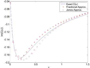
approximating functions have been developed: Ref. [5] gives an extensive but by no means exhaustive list. The vast majority of these approximations are rational functions in , as they have been designed for use in control loops where rational transfer functions are p efe able. We will consi e two app oximations to Theo o sen’s function in this wo : a rational representation of second order in the numerator and denominator, first given in [6]; and a fractional-order representation given in [7]. The use of the rational approximation will demonstrate that our methods can be used with any rational approximation to Theo o sen’s function an the use of the f actional app oximation will show also that our methods can be extended to more complex approximating functions than are widely used at present. We should note that fractional-order multiparameter eigenvalue problems have never been considered before, in neither practical nor theoretical literature. Our treatment of this problem opens up both an interesting area for future abstract research – the study of fractional multiparameter eigenvalue problems – and a wider class of fractional-order systems for use by practical modellers.

The rational approximation given by Jones [6] is

( )

(2.3.18)

with

(2.3.19)

Consider Eq. 2.3.10. Substituting Eq. 2.3.14 and multiplying by ( ), we obtain

(( ) ( ) ( )

( ) ( )

( ) ( ) )

(2.3.20)

(34)

(

)

(2.3.21) with

(2.3.22)

Eq. 2.3.21 is a fourth-order polynomial multiparameter eigenvalue problem. We develop a direct solver for this problem in Chapter 4.

The app oximation to Theo o sen’s function iven by Swinney [7] is

( ) ( )

( ) (2.3.23)

with

(2.3.24)

Substituting Eq. 2.3.23 into Eq. 2.3.10, multiplying by ( ( ) ), and expanding

( ) we obtain

(( ( )( ) ( ) ( )

( )) ( )

( ) )

(2.3.25)

(35)

(( ( ) ( ) ₍ ₎

₍ ₎ ₎

₎

(2.3.26)

To make further progress we specify ⁄ , which yields:

(( ( ) ( ) ( )

( ) )

)

(2.3.27)

Let us then define a new eigenvalue variable ̂ √ , in which case the system becomes

(( ̂ ₍ _{) ̂} ₍ ₎ _̂ ₍ ₎

̂ ₍ _{) ̂} _{) ̂}

̂ _̂ _̂ ₎

(2.3.28)

and simplifies to

( ̂ _̂ _̂ _̂ _̂ _̂

̂ _̂ _̂ ₎ (2.3.29)

with

( )

(36)

Eq. 2.3.29 is a polynomial multi-parameter eigenvalue problem of degree in ̂ and degree in . We develop a direct solver for this problem in Chapter 4.

2.3.6 Parameter values

In our derivation so far we have not yet specified the values of the structural and aerodynamic parameters in Eq. 2.3.11. We devise this model to be as close as possible to the introductory model (Section 2.2) but of course with damping and unsteady effects still included. Table 2.3 presents the extra model parameters (dimensional and nondimensional) not specified in Tables .1 an . . ote that even thou h Theo o sen’s ae o ynamic model is significantly more complex than the original steady model, no further aerodynamic parameters need be specified.

Table 2.3: Extra parameters for damped models

bending damp. coeff. – s m torsional damp. coeff. – ms a bending damp. ratio – torsional damp. ratio –

2.4 REFERENCES

[1] Hodges, D. H., and Pierce, G. A., 2011, Introduction to Structural Dynamics and Aeroelasticity, Cambridge University Press, New York, New York State, USA.

[2] Abramowitz, M., and Stegun, I., 1972, Handbook of Mathematical Functions, National Bureau of Standards, Washington D.C., USA.

[3] White, F. M., 2009, Fluid mechanics, McGraw-Hill, New York, New York State, USA. [4] Bisplinghoff, R. L., Ashley, H., and Halfman, R. L., 1957, Aeroelasticity, Addison-Wesley,

Reading, Massachusetts, USA.

[5] B unton S. L. an Rowley C. W. 013 “Empi ical state-space representations for Theo o sen’s lift mo el ” Jou nal of Flui s an St uctu es 38, pp. 174–186.

[6] Jones, R., 1938, Operational treatment of the nonuniform-lift theory in airplane dynamics, National Advisory Committee for Aeronautics, Washington D.C., USA.

(37)

Chapter 3 Visualisation methods

3.1 THE PURPOSE OF VISUALISATION METHODS

Visualisation methods allow us to visualise flutter points – their locations, relation to one another, nature and cause. This is in contrast to many direct and iterative solution methods, which supply the locations of the flutter points but nothing more. Visualisation methods are inevitably based on some form of enumeration procedure – solving a simple problem or evaluating a function over a grid of points. The results from this enumeration are then plotted, and the flutter points typically manifest themselves as some form of intersection. Visualisation methods can of course be used to provide reasonable numerical estimates of the location of the flutter points – for example by an interpolative procedure – but their main benefit is in providing contextual information. They provide information about the subcritical and supercritical dynamics of the system – below and above the flutter point, respectively. This information can be used to deduce the mechanisms leading to the creation of a flutter point, and these mechanisms may in turn inform aircraft design decisions.

(38)

Chapter 3 – page 29 3.2 MODAL DAMPING AND ROOT LOCUS

The modal damping and root locus methods are widely used to analyse stability problems. These methods do not need to be understood in the context of multiparameter eigenvalue problems. Consider a general eigenvalue problem, representing an aeroelastic system:

( ) (3.2.1)

The eigenvalue parameter is , representing the modal frequency of the structure, and

is another parameter which is some function of airspeed and modal frequency (e.g. airspeed itself, or the reduced frequency ⁄ ). We define a set of -values { } that are of interest, and at these values we solve the one-parameter eigenvalue problem for . The result is a set of solutions { } , for each element in { }. Note that, even if the dependency of on is too complex for standard solvers, the solution can always be determined with further enumeration: for each , we select a set of test points in complex space, { } at which we evaluate ( ). We then interpolate the resulting determinant field to such that ( ( )) . These points are the eigenvalues { } . However, it should also be noted that this process is extremely expensive, as it adds an extra two dimensions ( ( ) and ( )) to the normal one-dimensional search over .

(39)

applications [1–3]. Figure 3.1 shows an example of modal damping plot and corresponding frequency plot.

Figure 3.1: An example modal damping plot

The root locus method plots ({ } ) against ({ } ) for each eigenvalue. This has the advantage of fitting on a single plot, but it gives no direct graphical information about the dependency of the eigenvalues on the parameter . This information has to be determined by looking at the raw numerical data. Figure 3.2 shows an example root-locus plot. Note that in our root locus plots, the lower-half plane is the unstable half-plane. This is due to the definition of our eigenvalue (cf. Ch. 1 Sect. 1.1). In most aeroelastic applications, the modal damping plot is more widespread than the root locus plot, as the latter does not give any indication of the location of the flutter points in with respect to the parameter . However, it is still used [4,5].

(40)

standard (usually polynomial) eigenvalue solver. We did note that the use of a further enumeration / interpolation procedure be used for a more general system, but this procedure is seldom feasible due to the high computational expense.

Figure 3.2: An example root locus plot

If we look back at the multiparameter formulation of our flutter problem, Eq. 3.2.1, where

(41)

to the standard methods by the fact that the complex components of – whether is airspeed, reduced frequency, or some other parameter – are more difficult to interpret physically than the complex components of . However, there are some areas in which the reverse methods may be useful. Firstly, they do overcome the deficiency of the standard modal damping / root locus methods that was raised earlier. They work for an arbitrary continuous dependence of Eq. 3.2.1 on . But they replace this with another deficiency: they now rely on this equation having a sufficiently simple dependence on , because this is now the variable being solved for at each given . Unfortunately, the dependence of Eq. 3.2.1 on (no matter what airspeed parameter represents) is usually more complex that its dependence on , so that the standard methods will usually be more practical than the reverse ones. However, there are some cases where the reverse methods may be practical. For example, the flutter analysis of long-span bridges is often carried out with experimental aerodynamic models base on flutter derivative parameters [6–8]. If these flutter derivatives are not allowed to vary with airspeed, then the Eq. 3.2.1 becomes quadratic with respect to airspeed. If this is so, then the reverse root locus methods allow for an arbitrary continuous dependence of Eq. 3.2.1 – for example, viscoelastic effects could be included in the problem with essentially no added computational time. However, it is questionable whether a model based on constant flutter derivatives would be accurate enough to be industrially relevant, as these derivatives usually vary [6–8].

If a system with sufficiently simple dependence on is found, then the reverse methods offer quite a different perspective into the behaviour of the system than the standard ones. This is simply a result of the nature of the initial set of points of interest, { } or { }. The standard methods will compute all the flutter points (at any mode) over a given airspeed range (the range of { }). The reverse methods will compute all the flutter points over the given frequency range (the range of { }). Figure 3.5 indicates this difference, on a plot of

(42)

Chapter 3 – page 33 Figure 3.3: An example reverse root locus plot

(43)

Figure 3.5: Solution zones for standard and reverse modal damping plots.

One thing that should be noted about the reverse methods is that it is impossible to distinguish a destabilisation event (modal damping changing from positive to negative) from a restabilisation even (modal damping changing from negative to positive). While it may be possible to do so, the author has not yet found a relationship between the imaginary and the modal damping that would allow one to make such a distinction. Hence our reverse methods will only locate points on the flutter boundary, and will not describe their nature. However in standard aeroelastic analysis this is not a problem for two reasons. Firstly, because in a physical aeroelastic system we should expect the restabilisation to always occur at higher airspeeds than the destabilisation. Making this assumption, it is easy to distinguish these two points (along any given modal line, we will have a series of alternating restabilisations and destabilisations). Secondly, because the restabilisation points are of no known industrial relevance anyway. Aeroelastic engineers do not usually deal with structures that are unstable at zero airspeed and then stabilise once the aircraft is moving.

(44)

Chapter 3 – page 35 3.3 CONTOUR PLOT

When we devised the reverse modal damping / root locus methods, we were essentially adapting existing methods to a multiparameter context. However, with some consideration we can devise a more powerful method which does not reference these existing modal damping / root locus techniques. Consider again the original eigenvalue problem:

( ) (3.3.1)

If and , then a solution only exists on the stability boundary, and nowhere else. However, ( ( )) does exist over [ ] . The eigenvalues of the system will be the roots of the determinant:

( ( )) (3.3.2)

In general, ( ( )) . Hence Eq. 2.3 is equivalent to specifying

( ( ( )))

( ( ( ))) (3.3.3)

Eq. 3.3.3 defines two sets of contours over [ ] . The flutter points are the intersections of these two sets of contours. Dynamic flutter points are intersections that occur at nonzero , and divergence points are intersections occurring theoretically at ; but due to the inevitable numerical errors in the interpolation of these intersections, they will appear at small negative or positive . The procedure for determining the flutter points is thus as follows:

1. Define a grid of points {[ ]} 2. Evaluate the complex ( ( ))

3. Plot the contours of ( ) and ( ) .

(45)

Chapter 3 – page 36 Figure 3.6: An example contour plot

The most significant advantage of this method is its applicability to unstructured systems – that is, for which neither variable can be solved with a direct solver. We saw earlier that the modal damping / root locus methods are capable of handling such system, but at the expense of requiring three enumerations in total: the initial { } , and then { } (that is, { ( )} and { ( )} ). The contour plot requires only two enumerations: { } and { } . We have removed a whole dimension from the search space.

(46)

undamped natural frequencies and the real contours is more subtle. These undamped natural frequencies are the lines of ( ( )) , whereas the real contours are

( ( )) . The difference is that in general ( ( )) ( ( )) for complex . At the flutter points, the damped natural frequencies are equivalent to the real contours. This is self-evident: at the flutter points and ( ) so the two definitions merge. The undamped natural frequencies are not equivalent, because the fact that ( ) does not imply ( ( )) for complex . Of course, if the system is entirely undamped1 then the damped and undamped natural frequencies coalesce, and we can easily show that the real contours are equivalent to this coalesced natural frequency. Firstly, we define the system ( ) as being undamped if:

[ ] ( ) (3.3.4)

That is, is never complex-valued for any real or . In a polynomial matrices system this is equivalent to all the matrix coefficients being real. The natural frequencies of such a system (for given ) are the eigenvalues, ( ( )) . If Eq. 3.3.4 holds, then

( ( )) and hence ( ( ( ))) ( ( )). That is, the real contours are equivalent to the natural frequencies of the structure as a function of .

While we have not proved any error bounds, numerical experimentation indicates that the real contours in the contour plots are good approximations of the natural frequencies of modes with low modal damping. We present some of these experiments in Section 3.4. This makes the contour plot method particularly attractive for visualising systems formulated using the pk-method: the pk-method only produces good approximations of the modal behaviour in the lightly-damped modes anyway.

1

(47)

Chapter 3 – page 38 3.4 NUMERICAL EXPERIMENTS

3.4.1 Simple section model

To begin our numerical experiments we will consider the introductory model described in Chapter 2:

( ) (3.4.1)

The purpose of experimenting with this system is to validate the most basic methods that we will be using – the modal damping and root locus plots – and to show that our methods are capable of replicating established results. Ironically, this system is one of the most troublesome to analyse by the methods we will look at in this thesis, and serves to illustrate the complexity that even simple systems can pose.

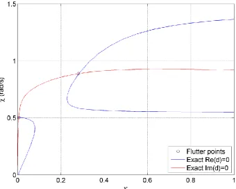
Figure 3.6 shows a modal damping plot for this system. There are two aeroelastic events over the simulated airspeed range: a flutter point and then a divergence point. We locate the divergence point at approximately and the flutter point at and

. The divergence point agrees very well with the analytical solution obtained in [2], namely . The flutter point matches well with the value obtained numerically in [2], which is and (see Chapter 2). This validates our implementation of the modal damping method. We can then compare this solution to that of the other methods. Figure 3.7 shows a root locus plot for this system. The plot gives no direct graphical information as to the location of the flutter and divergence points in , but the flutter frequency can be observed to be . The problematic aspect of this system can be seen in Figure 3.6: the system has zero modal damping for all airspeeds apart from the gap at . Every airspeed outside this gap is technically a flutter point, as it has a neutral stability. Hence the multiparameter problem of determining the flutter points of the system has a continuous spectrum. We can see this when we consider the contour plot of this system (Figure 3.8). Note that ( ) is identically zero everywhere. Every point outside the range

(48)

Chapter 3 – page 39 Figure 3.6: Modal damping plot for introductory system

(49)

Figure 3.8: Contour plot of introductory system. The imaginary part of the determinant is zero everywhere.

3.4.2 Undamped section model with quasisteady aerodynamics

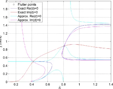
We now simulate a more complex model: the section model with quasisteady Theodorsen aerodynamics and no structural damping (Eq. 3.4.2).

(( ) ( ) ) (3.4.2)

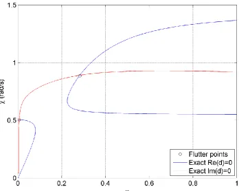
Figure 3.9 shows a contour plot of this system. The plot range covers both positive and negative , so that its symmetry may be appreciated. According to this contour plot, the flutter point is located at , . One non-physical flutter point can be located at , and two other points of neutral stability at and

(50)

Figure 3.9: Contour plot for the section model with quasisteady Theodorsen aerodynamics and no structural damping

(51)

To validate this contour plot, we produce a modal damping plot. Figure 3.10 shows such a plot. Flutter can be seen to occur at . We can link the modal damping curve for this flutter point with the lower modal frequency path in the ( ) plot – though this is not obvious from the plot, and we have to investigate the raw data to determine this. We thus can estimate that ( ). The two points of neutral stability lie at , and ( and

). This agrees well with the contour plot.

3.4.3 Section model with quasisteady aerodynamics

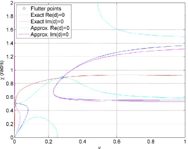
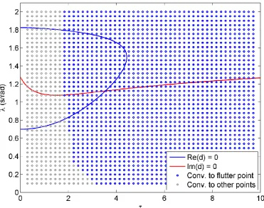
As an extension of Section 3.4.2, we simulate the quasisteady section model with structural damping now included. This is a system which could be industrially useful to visualise. In Chapter 2 we presented two forms of this system: the form in - and the form in - . In this section we solve both forms, and compare them to the undamped quasistatic section model (Section 2.4.2) and the introductory model (Section 2.4.1) respectively. Consider first the - form:

(( ) ( ) ) (3.4.3)

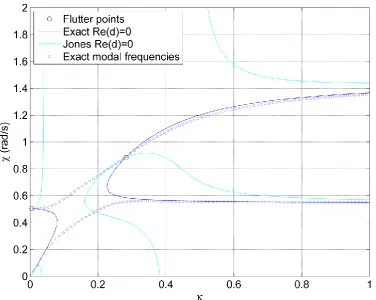
Figure 3.11 shows the contour plot for the damped quasisteady system, superimposed on the contour plot for the undamped quasisteady system (mapped from to ). As can be seen, the real contours for these two plots are practically identical. The imaginary contours are similar in general trend, but the damped imaginary contours are now apparently hyperbolic in nature (though in fact they are quartic plane curves). Note that the symmetry of the plot is now broken. The physical flutter point in Figure 3.11 can be located at

(52)

Figure 3.11: Comparison between the contour plots of the damped and undamped quasisteady system.

Consider now the - form of the system:

(( ) ( ) ) (3.4.4)

Figure 3.12 shows a modal damping plot for this system, superimposed on that of the steady introductory model (see Section 2.4.1). The flutter point for the damped model in Figure 3.12 can be located at . From the raw data we can link the associated modal damping curve with the upper modal frequency path in the ( ) plot, and hence we estimate that . This corresponds to and , agreeing with the results from the - form. The divergence point can be located at