Munich Personal RePEc Archive
What do the shadow rates tell us about
future inflation?
Kuusela, Annika and Hännikäinen, Jari
University of Jyväskylä, University of Tampere
1 August 2017
What do the shadow rates tell us about future
inflation?
∗
Annika Kuusela
†School of Business and Economics, University of Jyv¨askyl¨a
Jari H¨annik¨ainen
‡School of Management, University of Tampere
Abstract
This paper investigates whether shadow interest rates contain predictive power
for U.S. inflation in a data-rich environment. We find that shadow rates are useful
leading indicators of inflation. Shadow rates contain substantial in-sample and
out-of-sample predictive power for inflation in both the zero lower bound (ZLB)
and non-ZLB periods. We find that the shadow rate suggested by Wu and Xia
(2016) contains more information about future inflation than the shadow rate
suggested by Krippner (2015b).
Keywords: shadow interest rates, zero lower bound, unconventional
mone-tary policy, inflation forecasting, data-rich environment, factor models
JEL codes: C38, C53, E37, E43, E44, E58
∗We would like to thank Kari Heimonen, Ari Hyytinen, Tomi Kortela, Leo Krippner, Antti Ripatti, and the participants of the FDPE Econometrics workshop for helpful comments and suggestions and Leo Krippner for providing Matlab codes. Financial support from the OP Group Research Foundation and Jyv¨askyl¨a International Macro & Finance Research Group is gratefully acknowledged.
1.
Introduction
During the recent global financial crisis central banks around the world, including the
Federal Reserve (Fed), have cut interest rates to near zero and introduced
unconven-tional monetary policy measures such as quantitative easing and forward guidance.1
These measures have been useful in easing the economic conditions as the primary
mon-etary policy instrument, the short-term nominal interest rate, has been constrained by
the zero lower bound (ZLB).2 When policy rates are in the ZLB range for a prolonged
period of time, the stance of the Fed’s monetary policy cannot be evaluated by the
observable variations of the federal funds rate. This has raised the question of how to
measure the overall stance of the monetary policy in the ZLB environment.
One possible way to approach this question is to consider longer maturity interest
rates. They can be seen as a proxy for the policy rate, but they are not constrained by
the ZLB. They are also influenced by current and expected short-term interest rates.
Thus, several researchers (e.g., Krippner 2015b; Wu and Xia 2016) have used
longer-term interest rates to construct a shadow (short) rate using a longer-term structure model.
The shadow rate is a quantitative measure that indicates the overall stance of the
monetary policy when the conventional monetary policy instrument (the short-term
policy rate) is at the ZLB. It takes into account the effects of unconventional monetary
policy actions and can freely take on negative values in the ZLB environment. The
shadow rate is the shortest maturity from the estimated shadow yield curve. In the
non-ZLB environment the shadow rate is essentially equal to the policy rate.
The previous shadow rate literature has mostly focused on modeling the shadow
rates, discussing the sensitivity of the shadow rate estimates, and analyzing the
con-1
For comprehensive analysis of unconventional monetary policy measures, see, e.g., Bernanke et al. (2004) and their effectiveness, see, e.g., Neely (2015) and the references cited therein.
2
sistency of shadow rate movements with unconventional monetary policy actions. Kim
and Singlenton (2012) estimated several two-factor models using Japanese Government
Bond yields. They found that shadow rate models capture the variation in bond yields
during periods of near-zero short-term rates. Christensen and Rudebusch (2015)
de-rived an option-based approach to estimated one-, two-, and three-factor models and
showed the sensitivity of the shadow rate estimates to the model fit and specification.
Bauer and Rudebusch (2016) forecasted the expected time to the policy rate lift-off
and how long the policy rate will remain near zero with U.S. data.
This paper contributes to the existing literature by examining whether the shadow
rates contain predictive power for U.S. inflation. It is well known that monetary policy
affects future inflation and thus the shadow rates, as measures of the stance of monetary
policy in the ZLB period are potentially useful leading indicators of inflation. Chung
et al. (2012) and Mishkin (2017) point out that ZLB periods can be more frequent
and long-lasting than the standard macro literature has suggested. The standard
macro models have underestimated the incidence and effects of ZLB events, because
contractionary shocks may appear more frequently than previously anticipated and
lead to ZLB constraint binding more often. That is, the ZLB periods have become
more significant to the central banks than was foreseen before the recent financial
crisis. Therefore investigating the indicator properties of the shadow rates in the ZLB
environment is essential.
We analyze the in-sample and out-of-sample predictive power of the shadow rates
in a data-rich environment using factor models. We investigate whether the predictive
power remains stable over time and especially whether the shadow rates contain
pre-dictive power in the recent ZLB/unconventional monetary policy era. To the best of
our knowledge, the extant literature has not analyzed the relationship between shadow
rates and future inflation in a systematic way.3 Thereby, our paper is intended to
3
bridge this gap.
We consider shadow rates estimated by two alternative term structure models. The
first is the shadow rate term structure model by Wu and Xia (2016) (henceforth WX),
which is a three-factor model, and the other is the Krippner arbitrage-free Nelson
and Siegel (1987) model with two state-variables by Krippner (2015b) (henceforth
K-ANSM). Because Bauer and Rudebusch (2016) and Krippner (2015a) show that the
estimated shadow rates are very sensitive to the selected values of the lower bound
parameter, we carefully analyze the robustness of our forecasting results. To implement
this we use four different lower bound parameter values for both the WX and the
K-ANSM shadow rates. We also analyze whether the results remain robust when the
sample period used in the estimation of the shadow rates is changed.
The main finding from this study is that the shadow rates are useful leading
indi-cators of U.S. inflation. Shadow rates contain substantial predictive power for inflation
both in the non-ZLB and ZLB periods irrespective of which model specification or
forecast horizon is considered. We find that the shadow rate suggested by Wu and
Xia (2016) produces more accurate inflation forecasts than the shadow rate suggested
by Krippner (2015b), probably because it fits better to the yield curve data and thus
contains more information. Our results are robust regardless of the lower bound
pa-rameter or the estimation period considered. We believe that our results are important
for forecasters, central banks and other policymakers, because it has been difficult to
find good leading indicators for inflation in the post-1985 period (see, e.g., Stock and
Watson 2003; 2007).
The remainder of the paper is organized as follows. Section 2 describes the
method-ology. Section 3 introduces the data used for the estimations. Section 4 presents the
results of the in-sample and out-of-sample forecasting exercises. Section 5 concludes.
Appendix A at the end of the paper provides a detailed description of the dataset.
2.
Methodology
In this section, we describe the econometric methodologies used in this paper. The
purpose of this study is to evaluate whether different shadow rates contain predictive
power for U.S. inflation. To this end, we conduct both in-sample and out-of-sample
forecasting exercises.
We examine the predictive content of shadow rates in a data-rich environment. We
use factor models, because they provide a parsimonious way of dealing with a large set
of candidate predictors. The key insight of factor models is that predictor variables
are often strongly correlated, and thus, the information encoded in a large number of
candidate predictors can be summarized by a handful of unobserved factors. These
factors can be consistently estimated by principal components (Stock and Watson,
2002a). Factor models have become popular in macroeconomic analysis in recent years,
especially when the focus is on forecasting.4
To assess the predictive ability of shadow rates, we estimate the following linear
h-step-ahead factor model (henceforth, the shadow rate forecasting model):
πth+h =αh+ m
X
j=1
k
X
i=1
βhijFi,tˆ −j+1+
p
X
j=1
γhjπt−j+1+φhzt+ε
h
t+h, (1)
where the dependent variable and the lagged dependent variable are πh
t+h = (1200/h) ln(Pt+h/Pt) andπt = 400ln(Pt/Pt−1), respectively,Ptis the price index at month t, ˆFi,t
is the ith principal component constructed from a large set of predictors, zt is either
the WX or K-ANSM shadow rate, and εh
t+h is the forecast error. The constant term
is included in the forecasting regression (1), and the superscripts h indicate that the
parameters are horizon specific.
Forecasts of consumer price index (CPI) inflation and personal consumption
ex-4
penditures (PCE) inflation are generated for horizons of h = 3, 6, 9, and 12 months.
The factors are extracted by principal components, and the forecasting regression (1)
is estimated by OLS. The lags of factorsm, the number of factorsk, and the number of
autoregressive lags pof each specification are determined by the Bayesian information
criterion (BIC), with 1≤ m≤ 2, 1≤ k ≤4, and 0≤p ≤6. The error term in model (1) is autocorrelated, because the sampling interval is smaller than the forecasting
hori-zon. The MA (h-1) structure of the error term induced by overlapping observations is
taken into account by computing Newey and West (1987) HAC standard errors with
the lag truncation parameter equal to h - 1.
Furthermore, we are interested in whether the beginning of the ZLB period changed
the relationship between the shadow rates and future inflation. To address this
ques-tion, we create a dummy variable that takes a value of one when the federal funds
rate is at the ZLB (2009:M1–2015:M12) and zero otherwise. To study the differences
between the non-ZLB and ZLB periods, an interaction term that is the product of
the ZLB dummy and a shadow rate is included in the estimation, i.e., we consider a
predictive model of the form:
πht+h =αh+ m
X
j=1
k
X
i=1
βhijFi,tˆ −j+1+
p
X
j=1
γhjπt−j+1+φhzt+ψh(ZLBt∗zt) +ε
h
t+h, (2)
whereZLBt denotes the ZLB dummy.
Our main interest lies in the interaction coefficient ψh that captures the effects of
the ZLB/unconventional monetary policy environment on the relationship between the
shadow rates and future inflation. If the coefficient turns out to be insignificant, the
relation between the shadow rate and future inflation is similar in both periods. On
the other hand, a statistically significant coefficient implies that the relationship has
changed since the beginning of the ZLB/unconventional monetary policy period.
out-of-sample forecasting exercise. The out-out-of-sample forecasting period runs from October
1996 to December 2015. The model selection and estimation is recursive as the
fore-casting exercise proceeds through time. That is, we extract the factors and estimate the
parameters of the forecasting model (1) using all available prior data at each forecast
origin. The lags of factorsm, the number of factorsk, and the number of autoregressive
lagsp are determined by the data, with 1≤m≤2, 1≤k ≤4 and 0≤p≤6. At each forecast origin we select the model with the lowest BIC.
We quantify out-of-sample performance by comparing the forecasting accuracy of
a shadow rate forecasting model relative to that of a benchmark model. In our
frame-work, natural benchmark models are obtained by excluding the shadow rate from the
forecasting model (1). By comparing the accuracy of the model augmented with a
shadow rate and the benchmark model, we investigate the marginal predictive power
of the shadow rate. The results in the previous literature show that factor models
typ-ically produce better macroeconomic forecasts than other popular forecasting models,
such as autoregressive or vector autoregressive models (see, e.g., Bernanke and Boivin
2003; Clements 2016; Stock and Watson 2002a,b). As a consequence, factor models
provide a stiff benchmark against which to compare the shadow rate forecasting model.
To facilitate comparisons between the shadow rate forecasting model and the
bench-mark model, we report the results in terms of their relative mean squared forecast error
(MSFE), which is the ratio of the MSFE from the shadow rate forecasting model over
the MSFE from the benchmark. The values of the relative MSFE below (above) unity
indicate that the shadow rate forecasting model produces more (less) accurate forecasts
than the benchmark model, implying that the shadow rate contains (does not contain)
marginal predictive power. To assess the statistical significance of improvements in
forecast accuracy relative to the benchmark model, we employ the one-sided Diebold
by Harvey et al. (1997).5
In addition, we report the fraction of observations for which the shadow rate
fore-casting model produces a smaller absolute forecast error than the benchmark model.
This exercise allows us to analyze whether the shadow rate forecasting model
qualita-tively outperforms the benchmark model. This is an important robustness check. As
is well known, the MSFE measure gives more weight to large errors. Therefore, the
MSFE results might give a misleading picture of the true predictive power in the
pres-ence of a few extreme forecast errors. On the other hand, the sign statistic gives equal
weight to each observation and is thus less sensitive to outliers. We test whether the
fraction of observations for which the shadow rate forecasting model generates a more
accurate forecast is statistically significantly above 0.5 using the sign test developed
by Diebold and Mariano (1995).
3.
Data
Our data consist of monthly observations of macroeconomic variables and shadow rates
from November 1985 to December 2015. We use CPI inflation and PCE inflation from
the Federal Reserve Bank of St. Louis FRED Economic database and measure inflation
by the annualized rate of inflation.6 We also use macroeconomic data from the
FRED-MD database, which includes 133 macroeconomic variables to create the factors in
5
Our forecasting models are nested in the sense that the benchmark model is a restricted version of the shadow rate forecasting model (1). The DM test is not designed for nested model comparison. We are aware of the limitations of the DM approach. However, our use of the DM test is a deliberate choice. The Monte Carlo results in Clark and McCracken (2013) indicate that the DM test with the small sample correction suggested by Harvey et al. (1997) provide a good sided test of the null hypothesis of equal finite-sample forecast accuracy even when the models are nested. Faust and Wright (2013) and Groen et al. (2013) also use the DM test when comparing inflation forecasts from nested models.
6
forecasting regressions (1) and (2).7 The FRED-MD database includes variables from
several categories, such as inflation, exchange rates, stock prices, and employment.8 We
estimate four factors from the FRED-MD database by principal components. The first
factor captures the variation of real activity and employment variables. The second
factor catches forward-looking variables, such as interest rate spreads and inventories.
The third factor can be interpreted as an inflation factor, because it associates with
price variables. The fourth factor captures the variation of a mix of housing and interest
rate variables. Typically BIC chooses a model that contains three factors.
We use 14 different shadow rates estimated from two different shadow (short) rate
models:
1. Shadow rate term structure model by Wu and Xia (2016) (WX)
2. Krippner arbitrage-free Nelson and Siegel (1987) model with two state-variables
(level and slope) by Krippner (2015b) (K-ANSM)
The WX model has already become a widely used model to summarize the overall
stance of monetary policy.9 It uses three factors to estimate the shadow rates, but
the problem with three-factor shadow rate estimates is that they do not correlate well
with unconventional monetary policy announcements and sometimes produce
counter-intuitive positive values during unconventional monetary policy periods. They are also
very sensitive to precise model specification, creating very different magnitudes and
profiles for minor changes in the lower bound specification. The problems related to
the WX model are discussed in more detail in Krippner (2015a). Krippner (2015a)
also shows that shadow rate estimates from a two-factor model are more suitable for
7
The FRED-MD database consists originally of 134 variables, but we have excluded variable num-ber 64 (New Orders for Consumer Goods) from the original database to get the balanced panel that we need for estimating the principal components. We have also standardized and stationarized the variables so that their sample mean is equal to zero and sample variance is equal to one. See Appendix A for a data description and Figure A1 for factors over time.
8
See McCracken and Ng (2016) for details of the FRED-MD database.
9
The WX shadow rate is published at the Federal Reserve Bank of Atlanta website: https :
describing the stance of monetary policy, because they correlate well with the
uncon-ventional monetary policy announcements and are relatively robust, producing similar
magnitudes and profiles. The advantage of the WX model is that it fits better to the
yield curve data used in estimating the shadow rates, especially at the short end, than
the K-ANSM model.
To estimate the WX shadow rates we construct monthly forward rates for maturities
of 0.25, 0.5, 1, 2, 5, 7, and 10 years using the G¨urkaynak et al. (2007) dataset10 and
observations at the end of the month. Our sample period for the forward rate data is
from January 1990 to December 2015. For the period from November 1985 to December
1989 we use the federal funds rate as the WX shadow rate. For K-ANSM shadow rates
we use the same G¨urkaynak et al. (2007) dataset as before for maturities 1, 2, 3,
5, 7, and 10 years and 3-month and 6-month T-bill rates from the FRED database
to calculate the continuously compounding T-bill rates for the short end of the yield
curve.11
For both shadow rate models we use four different lower bound (LB) parameters
and four different estimation periods. The WX shadow rates that we use are LB =
0, 14, 19, and 25 bps, and estimation periods end at December 2013 (Dec-13), April
2014 (Apr-14), December 2014 (Dec-14), and December 2015 (Dec-15). For K-ANSM
shadow rates we use LB = 0, 14, 16, and 25 bps and the same estimation periods as
for the WX shadow rates.12 These are chosen according to Krippner (2015a) except
that we have replaced the Sep-15 shadow rate with the Dec-15 shadow rate to obtain
a full sample for 2015.
Because the Federal Open Market Committee (FOMC) lowered the target range
for the federal funds rate to 0–25 bps in December 2008, we refer the period from
10
This dataset is available at
http://www.f ederalreserve.gov/pubs/f eds/2006/200628/200628abs.html
11
For a similar approach, see Krippner (2015a).
12
January 2009 to the end of our sample as the ZLB period. The shadow rates are
highly correlated and receive almost identical values in the non-ZLB period. Therefore
Figure 1 plots the shadow rates merely over the 2008:1–2015:M12 period. An inspection
of Figure 1 reveals that the shadow rate models are very sensitive to the LB parameters
and data used for the estimation. Figure 1 also shows that the WX shadow rates are
Figure 1: The shadow rates and federal funds rate
WX shado
w r
ate (%)
2008 2010 2012 2014 2016
−6
−4
−2
0
2
LB = 0 LB = 14 LB = 19 LB = 25 Fed funds
K−ANSM shado
w r
ate (%)
2008 2010 2012 2014 2016
−6
−4
−2
0
2
LB = 0 LB = 14 LB = 16 LB = 25 Fed funds
WX shado
w r
ate (%)
2008 2010 2012 2014 2016
−6 −4 −2 0 2 Dec−13 Apr−14 Dec−14 Dec−15 Fed funds K−ANSM shado w r ate (%)
2008 2010 2012 2014 2016
−6 −4 −2 0 2 Dec−13 Apr−14 Dec−14 Dec−15 Fed funds
4.
Empirical results
This section presents the results of the in-sample and out-of-sample forecasting
exer-cises.
4.1.
In-sample analysis
In this section we examine the in-sample predictive power of shadow rates for U.S.
inflation. First, we consider the estimation results for the forecasting regression (1),
which are presented in Tables 1 and 2. We present the results for shadow rates with
different values of the LB parameter and for different estimation periods.
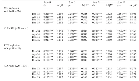
Tables 1 and 2 show that the relationship between the shadow rates and future
inflation is positive for all 14 shadow rates and for all four forecasting horizons.13 This
finding indicates that as the shadow rate decreases the future inflation also decreases.
All the shadow rate coefficients are statistically significant at the 1% level of
signif-icance. The LB specification or selection of the estimation period does not seem to
affect the results much.
The coefficients and adjustedR2s of the WX shadow rates are typically larger than
the coefficients and adjusted R2s of the K-ANSM shadow rates, especially when the
forecasting horizon is 9 or 12 months. These findings suggest that the WX shadow
rates perform better than the K-ANSM shadow rates in forecasting future inflation.
The LB parameter of 14 bps for the WX shadow rate and LB parameter of 0 bps for the
K-ANSM shadow rate give the highest adjusted R2s, which gives evidence that these
LB specifications could be the best predictors of inflation. The coefficient typically
increases as the forecasting horizon becomes longer, which supports the argument that
monetary policy affects inflation over a longer period of time. The adjusted explanation
ratios are higher for CPI inflation than for PCE inflation when the forecasting horizon
13
Table 1: In-sample predictive regressions
h= 3 h= 6 h= 9 h= 12
φ3 AdjR2 φ6 AdjR2 φ9 AdjR2 φ12 AdjR2 CPI inflation
WX
LB= 25 0.249*** 0.160 0.252*** 0.228 0.271*** 0.322 0.284*** 0.403 LB= 19 0.257*** 0.162 0.261*** 0.231 0.281*** 0.326 0.293*** 0.407 LB= 14 0.266*** 0.163 0.270*** 0.233 0.289*** 0.328 0.301*** 0.408 LB= 0 0.275*** 0.162 0.279*** 0.231 0.260*** 0.306 0.310*** 0.410
K-ANSM
LB= 25 0.221*** 0.151 0.212*** 0.202 0.198*** 0.263 0.228*** 0.345 LB= 16 0.238*** 0.153 0.229*** 0.206 0.211*** 0.268 0.245*** 0.352 LB= 14 0.242*** 0.154 0.232*** 0.207 0.214*** 0.269 0.248*** 0.353 LB= 0 0.266*** 0.158 0.256*** 0.213 0.233*** 0.277 0.271*** 0.362
PCE inflation
WX
LB= 25 0.202*** 0.189 0.200*** 0.228 0.209*** 0.288 0.205*** 0.327 LB= 19 0.209*** 0.191 0.207*** 0.230 0.216*** 0.292 0.212*** 0.331 LB= 14 0.215*** 0.192 0.213*** 0.233 0.223*** 0.294 0.216*** 0.342 LB= 0 0.223*** 0.191 0.222*** 0.231 0.231*** 0.291 0.224*** 0.340
K-ANSM
LB= 25 0.142*** 0.195 0.123*** 0.183 0.131*** 0.229 0.134*** 0.259 LB= 16 0.153*** 0.197 0.132*** 0.186 0.140*** 0.233 0.178*** 0.273 LB= 14 0.156*** 0.197 0.134*** 0.186 0.141*** 0.234 0.180*** 0.274 LB= 0 0.172*** 0.200 0.147*** 0.191 0.155*** 0.240 0.198*** 0.282
Notes: The in-sample forecasting period runs from 1985:M11 to 2015:M12. Asterisks denote statistical significance at the 1% (***), 5% (**), and 10% (*) levels, respectively.
is six months or longer.
The estimation results of the forecasting regression (2) are presented in Tables 3
and 4. Now we have added an interaction term to the forecasting regression to see if
the relationship between the shadow rates and future inflation is different between the
non-ZLB and ZLB periods. Table 3 shows that the coefficients of the interaction terms
for the WX shadow rates are positive and typically statistically significant when the
forecasting horizon is six months or longer. This finding indicates that the relationship
between the WX shadow rate and future inflation is positive in both periods, but the
relationship tends to be stronger in the ZLB period when the Fed conducts
uncon-ventional monetary policies. The coefficients of the interaction term for the K-ANSM
shadow rates are typically statistically insignificant, indicating that the relationship
between the shadow rate and future inflation is similar in both periods.
One possible explanation for our results is the forward-looking nature of monetary
policy.14 The positive relationship between the shadow rates and future inflation arises
probably because the Fed anticipates lower future inflation and reacts to this new
in-formation by decreasing the policy rate (or by using unconventional monetary policies
in the ZLB period). That is, we observe the shadow rate decreasing, because the Fed
predicts that inflation will decrease in the future.15 Monetary policy affects inflation
with a long lag. Thus, the impacts of (unconventional) monetary policy actions on
inflation probably do not show entirely within a short time period.16 Due to this, the
short-term (3–12 months) inflation can fall even though the Fed pursues an
accom-modative monetary policy. The reverse causality from inflation to the shadow rate
causes a positive correlation between these two variables in the short term.
14
Rearranging the variables in our forecasting regression gives us an expression that looks like a forward-looking Taylor rule.
15
Our results refer to the price puzzle (see, e.g., Sims 1992). Wu and Xia (2016) use the FAVAR model and obtain results similar to ours for the relationship between the policy rate and future inflation.
16
Table 2: In-sample predictive regressions (re-estimated shadow rates)
h= 3 h= 6 h= 9 h= 12
φ3 AdjR2 φ6 AdjR2 φ9 AdjR2 φ12 AdjR2 CPI inflation
WX (LB= 25)
Dec-13 0.249*** 0.160 0.252*** 0.228 0.271*** 0.322 0.284*** 0.403 Apr-14 0.240*** 0.164 0.244*** 0.236 0.261*** 0.332 0.273*** 0.414 Dec-14 0.228*** 0.167 0.231*** 0.240 0.246*** 0.336 0.256*** 0.419 Dec-15 0.240*** 0.162 0.243*** 0.232 0.262*** 0.328 0.274*** 0.410
K-ANSM (LB=est.)
Dec-13 0.238*** 0.153 0.229*** 0.206 0.211*** 0.268 0.245*** 0.352 Apr-14 0.238*** 0.153 0.228*** 0.206 0.210*** 0.268 0.244*** 0.352 Dec-14 0.241*** 0.154 0.232*** 0.207 0.213*** 0.269 0.248*** 0.353 Dec-15 0.241*** 0.154 0.231*** 0.207 0.213*** 0.269 0.248*** 0.353
PCE inflation
WX (LB= 25)
Dec-13 0.202*** 0.189 0.200*** 0.228 0.209*** 0.288 0.205*** 0.327 Apr-14 0.194*** 0.193 0.192*** 0.234 0.201*** 0.296 0.196*** 0.335 Dec-14 0.183*** 0.195 0.181*** 0.237 0.188*** 0.299 0.184*** 0.338 Dec-15 0.193*** 0.190 0.192*** 0.230 0.201*** 0.292 0.197*** 0.331
K-ANSM (LB=est.)
Dec-13 0.153*** 0.197 0.132*** 0.186 0.140*** 0.233 0.178*** 0.273 Apr-14 0.153*** 0.197 0.131*** 0.186 0.139*** 0.233 0.177*** 0.273 Dec-14 0.155*** 0.197 0.133*** 0.186 0.141*** 0.234 0.180*** 0.274 Dec-15 0.155*** 0.197 0.133*** 0.186 0.141*** 0.234 0.180*** 0.274
Notes: The in-sample forecasting period runs from 1985:M11 to 2015:M12. Asterisks denote statistical significance at the 1% (***), 5% (**), and 10% (*) levels, respectively.
Table 3: In-sample predictive regressions with interaction terms
h= 3 h= 6 h= 9 h= 12
φ3 ψ3 AdjR2 φ6 ψ6 AdjR2 φ9 ψ9 AdjR2 φ12 ψ12 AdjR2 CPI inflation
WX
LB= 25 0.195** 0.351 0.163 0.196** 0.362 0.236 0.219*** 0.343 0.332 0.233*** 0.334 0.415 LB= 19 0.193** 0.498 0.168 0.194** 0.522* 0.246 0.217*** 0.496** 0.345 0.233*** 0.473** 0.429 LB= 14 0.207*** 0.541 0.171 0.208*** 0.563** 0.251 0.233*** 0.511** 0.349 0.251*** 0.464** 0.430 LB= 0 0.225*** 0.799* 0.174 0.226*** 0.842*** 0.259 0.235*** 0.771*** 0.341 0.275*** 0.583*** 0.433
K-ANSM
LB= 25 0.326*** -0.375* 0.163 0.311*** -0.354* 0.222 0.296*** -0.342* 0.289 0.304*** -0.270 0.366 LB= 16 0.327*** -0.398 0.163 0.313*** -0.375* 0.222 0.299*** -0.361* 0.290 0.305*** -0.268 0.366 LB= 14 0.328*** -0.405 0.163 0.313*** -0.381* 0.222 0.299*** -0.366* 0.290 0.305*** -0.266 0.366 LB= 0 0.329*** -0.460 0.163 0.315*** -0.430 0.223 0.301*** -0.406 0.291 0.306*** -0.248 0.367
PCE inflation
WX
LB= 25 0.173*** 0.194 0.190 0.167*** 0.211 0.231 0.177*** 0.209 0.293 0.174*** 0.205 0.333 LB= 19 0.172*** 0.287 0.194 0.165*** 0.320 0.239 0.175*** 0.319* 0.304 0.173*** 0.306* 0.344 LB= 14 0.181*** 0.311 0.196 0.175*** 0.350* 0.244 0.186*** 0.337** 0.308 0.188*** 0.261* 0.351 LB= 0 0.192*** 0.498* 0.200 0.187*** 0.559*** 0.251 0.199*** 0.504*** 0.313 0.200*** 0.398*** 0.356
K-ANSM
LB= 25 0.211*** -0.236 0.203 0.198*** -0.254* 0.200 0.202*** -0.242 0.250 0.194*** -0.204 0.276 LB= 16 0.212*** -0.249 0.203 0.200*** -0.277 0.200 0.204*** -0.259 0.250 0.226*** -0.214 0.287 LB= 14 0.212*** -0.253 0.203 0.201*** -0.283 0.201 0.204*** -0.263 0.251 0.226*** -0.214 0.287 LB= 0 0.214*** -0.285 0.204 0.204*** -0.336 0.201 0.206*** -0.301 0.252 0.227*** -0.211 0.288
Notes: The in-sample forecasting period runs from 1985:M11 to 2015:M12. Asterisks denote statistical significance at the 1% (***), 5% (**), and 10% (*) levels, respectively.
Table 4: In-sample predictive regressions with interaction terms (re-estimated shadow rates)
h= 3 h= 6 h= 9 h= 12
φ3 ψ3 AdjR2 φ6 ψ6 AdjR2 φ9 ψ9 AdjR2 φ12 ψ12 AdjR2 CPI inflation
WX (LB= 25)
Dec-13 0.195** 0.351 0.163 0.196** 0.362 0.236 0.219*** 0.343 0.332 0.233*** 0.334 0.415 Apr-14 0.192** 0.222 0.166 0.192** 0.235 0.241 0.215*** 0.209 0.337 0.230*** 0.192 0.421 Dec-14 0.194** 0.116 0.166 0.195*** 0.122 0.241 0.218*** 0.094 0.337 0.234*** 0.076 0.419 Dec-15 0.204** 0.167 0.162 0.202*** 0.193 0.235 0.224*** 0.181 0.332 0.238*** 0.168 0.415
K-ANSM (LB=est.)
Dec-13 0.327*** -0.398 0.163 0.313*** -0.375* 0.222 0.299*** -0.361* 0.290 0.305*** -0.268 0.366 Apr-14 0.327*** -0.398* 0.163 0.313*** -0.375* 0.222 0.299*** -0.361* 0.290 0.305*** -0.267 0.366 Dec-14 0.328*** -0.404 0.163 0.313*** -0.380* 0.222 0.299*** -0.366* 0.290 0.305*** -0.266 0.366 Dec-15 0.327*** -0.404 0.163 0.313*** -0.381* 0.222 0.299*** -0.366* 0.290 0.305*** -0.266 0.366
PCE inflation
WX (LB= 25)
Dec-13 0.173*** 0.194 0.190 0.167*** 0.211 0.231 0.177*** 0.209 0.293 0.174*** 0.205 0.333 Apr-14 0.169*** 0.113 0.192 0.163*** 0.132 0.236 0.173*** 0.123 0.298 0.170*** 0.117 0.338 Dec-14 0.170*** 0.045 0.193 0.164*** 0.058 0.236 0.175*** 0.047 0.298 0.172*** 0.041 0.337 Dec-15 0.177*** 0.073 0.188 0.170*** 0.102 0.230 0.179*** 0.102 0.293 0.175*** 0.101 0.333
K-ANSM (LB=est.)
Dec-13 0.212*** -0.249 0.203 0.200*** -0.277 0.200 0.204*** -0.259 0.250 0.226*** -0.214 0.287 Apr-14 0.212*** -0.249 0.203 0.200*** -0.276 0.200 0.204*** -0.259 0.250 0.226*** -0.214 0.287 Dec-14 0.212*** -0.252 0.203 0.201*** -0.282 0.200 0.204*** -0.263 0.250 0.226*** -0.213 0.287 Dec-15 0.212*** -0.252 0.203 0.201*** -0.282 0.200 0.204*** -0.263 0.250 0.226*** -0.213 0.287
Notes: The in-sample forecasting period runs from 1985:M11 to 2015:M12. Asterisks denote statistical significance at the 1% (***), 5% (**), and 10% (*) levels, respectively.
4.2.
Out-of-sample forecasting results
Next, we present the results of the out-of-sample forecasting exercise outlined in Section
2. The aim of this exercise is to analyze (i) whether the shadow rates contain predictive
power for U.S. inflation in a data-rich environment, (ii) whether the choice of the LB
parameter matters for the predictive ability of the shadow rates, and (iii) whether the
results remain robust when the sample period used in the estimation of the shadow
rates is changed.
We start our analysis by considering the shadow rates estimated with data from
January 1990 to December 2013 (i.e., the shadow rates in the upper panel of Figure
1). The MSFE results for the whole 1996:M10–2015:M12 out-of-sample period are
summarized in Table 5. This table shows the MSFE value of the shadow rate forecasting
model relative to the MSFE value of the benchmark model.17 Values below (above)
unity indicate that the model augmented with a shadow rate has produced more (less)
accurate forecasts than the benchmark model, implying that the shadow rate contains
(does not contain) marginal predictive power. The statistical significance is evaluated
using the one-sided DM (1995) test with the small sample modification proposed by
Harvey et al. (1997).
Three main results emerge from Table 5. First, the relative MSFE values are
be-low one, indicating that the models augmented with the shadow rates produce more
accurate inflation forecasts than the benchmark models. The improvements in
fore-cast accuracy are typically large (up to 30%) and statistically significant for the WX
shadow rates. This result holds irrespective of which shadow rate or forecast horizon
is considered. Therefore, both the WX and K-ANSM shadow rates contain predictive
power for U.S. CPI and PCE inflation when the predictive information encoded in a
17
large number of macroeconomic variables is already taken into account. This is an
im-portant finding, because the results in the previous literature suggest that it is difficult
to find good leading indicators for inflation in the post-1985 period (see, e.g., Stock and
Watson 2007). Second, the WX shadow rates produce better out-of-sample forecasts
than the K-ANSM shadow rates. The relative MSFE values for the WX shadow rates
are lower than those for the K-ANSM shadow rates, sometimes by quite a substantial
margin. Indeed, for all dependent variable/forecast horizon combinations, the worst
performing WX shadow rate outperforms the most accurate K-ANSM shadow rate.
Third, the choice of the LB parameter does not matter much for the out-of-sample
forecasting performance. The relative MSFE values for all LB parameters are quite
similar. Thus, the best performing LB parameter makes only a very slight improvement
over the alternatives. The results suggest that the LB parameter of 14 bps performs
the best for the WX shadow rate, whereas the K-ANSM shadow rate with the LB
pa-rameter of 0 bps yields the most accurate forecasts (cf. the in-sample results in Section
4.1.).
Table 5 focuses on the average predictive power over the whole out-of-sample period.
However, the purpose of this study is to examine whether the shadow rates contain
predictive power in the recent ZLB/unconventional monetary policy era. To shed light
on this question, we divide the out-of-sample period into two parts. The non-ZLB
period runs from 1996:M10 to 2008:M12, and the ZLB period runs from 2009:M1
to 2015:M12. The results for these two subperiods are reported in tables 6 and 7,
respectively.
The results in Table 6 show that the WX and K-ANSM shadow rates have predictive
power for inflation in the non-ZLB period. The relative MSFE values are below one for
both measures of inflation regardless of which forecast horizon is considered. However,
Table 5: Relative out-of-sample MSFE values
h= 3 h= 6 h= 9 h= 12
CPI inflation
WX
LB= 25 0.945 0.865* 0.757* 0.709*
LB= 19 0.943 0.861* 0.750* 0.701**
LB= 14 0.941* 0.857* 0.744** 0.696**
LB= 0 0.943* 0.853* 0.747** 0.707** K-ANSM
LB= 25 0.982 0.918 0.847 0.880
LB= 16 0.978 0.914 0.838 0.862
LB= 14 0.977 0.912 0.836 0.859
LB= 0 0.970 0.900 0.822 0.838
PCE inflation
WX
LB= 25 0.926* 0.903* 0.846 0.830
LB= 19 0.924* 0.899* 0.842* 0.824
LB= 14 0.922* 0.896* 0.837* 0.819
LB= 0 0.922** 0.896* 0.835* 0.824* K-ANSM
LB= 25 0.990 0.971 0.935 0.890
LB= 16 0.984 0.968 0.926 0.883
LB= 14 0.983 0.966 0.923 0.882
LB= 0 0.974 0.962 0.910 0.870
Notes: The out-of-sample forecasting period runs from 1996:M10 to 2015:M12. Each row reports the ratio of the MSFE of the shadow rate forecasting model to the MSFE of the benchmark model. Asterisks mark rejection of the one-sided Diebold and Mariano (1995) test with the small sample modification by Harvey et al. (1997) at the 1% (***), 5% (**), and 10% (*) significance levels, respectively.
Table 6: Relative out-of-sample MSFE values for the non-ZLB period
h= 3 h= 6 h= 9 h= 12
CPI inflation
WX
LB= 25 0.989 0.924 0.865 0.829
LB= 19 0.989 0.924 0.865 0.830
LB= 14 0.989 0.924 0.865 0.830
LB= 0 0.989 0.924 0.865 0.830 K-ANSM
LB= 25 0.994 0.912 0.870 0.888
LB= 16 0.994 0.912 0.869 0.887
LB= 14 0.994 0.912 0.869 0.887
LB= 0 0.993 0.909 0.869 0.886
PCE inflation
WX
LB= 25 0.968 0.960 0.935 0.925
LB= 19 0.968 0.960 0.935 0.925
LB= 14 0.968 0.960 0.935 0.925
LB= 0 0.968 0.959 0.935 0.924 K-ANSM
LB= 25 0.999 0.976 0.970 0.943
LB= 16 0.999 0.980 0.969 0.942
LB= 14 0.999 0.980 0.969 0.942
LB= 0 0.999 0.979 0.967 0.940
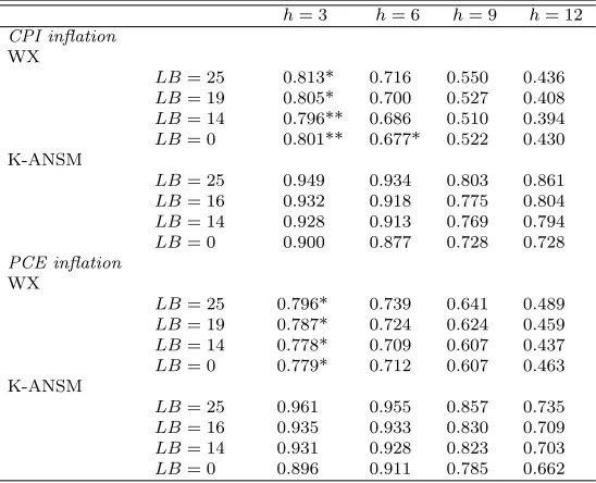
[image:22.612.88.355.433.658.2]Table 7: Relative out-of-sample MSFE values for the ZLB period
h= 3 h= 6 h= 9 h= 12
CPI inflation
WX
LB= 25 0.813* 0.716 0.550 0.436
LB= 19 0.805* 0.700 0.527 0.408
LB= 14 0.796** 0.686 0.510 0.394
LB= 0 0.801** 0.677* 0.522 0.430 K-ANSM
LB= 25 0.949 0.934 0.803 0.861
LB= 16 0.932 0.918 0.775 0.804
LB= 14 0.928 0.913 0.769 0.794
LB= 0 0.900 0.877 0.728 0.728
PCE inflation
WX
LB= 25 0.796* 0.739 0.641 0.489
LB= 19 0.787* 0.724 0.624 0.459
LB= 14 0.778* 0.709 0.607 0.437
LB= 0 0.779* 0.712 0.607 0.463 K-ANSM
LB= 25 0.961 0.955 0.857 0.735
LB= 16 0.935 0.933 0.830 0.709
LB= 14 0.931 0.928 0.823 0.703
LB= 0 0.896 0.911 0.785 0.662
Notes: The out-of-sample forecasting period runs from 2009:M1 to 2015:M12. Each row reports the ratio of the MSFE of the shadow rate forecasting model relative to the MSFE of the benchmark model. Asterisks mark rejection of the one-sided Diebold and Mariano (1995) test with the small sample modification by Harvey et al. (1997) at the 1% (***), 5% (**), and 10% (*) significance levels, respectively.
they are never statistically significant.18 The predictive ability of the shadow rates
seem to be similar. There is a simple explanation for this finding. As discussed in
Section 3, shadow rates are constructed such that they are strongly correlated and
display similar properties in the non-ZLB period. As a consequence, the WX and
K-ANSM shadow rates perform almost equally well in the non-ZLB period. For this
reason, in what follows we save space and focus exclusively on the ZLB period.
An examination of Table 7 leads us to a number of important observations regarding
the predictive ability of shadow rates. The most important finding is that both the
WX and K-ANSM shadow rates contain substantial predictive power for CPI and PCE
inflation in the ZLB period. The models augmented with the shadow rates produce
systematically smaller MSFE values than the benchmark forecasting models in all
18
cases.19 The improvements in forecast accuracy are especially large (up to 60%) at
longer forecast horizons (h= 9 and 12). Despite the large differences in the predictive
ability, the DM (1995) test rejects the null of equal forecast accuracy at conventional
significance levels only for the WX shadow rates at the shortest h = 3 horizon.20
Broadly speaking, these results support the conclusion of Wu and Xia (2016) that
shadow rates contain useful information about the state of the economy when the
short-term rates are stuck at the ZLB.21
Another important finding from Table 7 is that the WX shadow rates produce
more accurate inflation forecasts than the K-ANSM shadow rates in the
ZLB/un-conventional monetary policy environment. This result is a bit surprising. Krippner
(2015a) shows that the K-ANSM shadow rates are better suited for monitoring the
stance of unconventional monetary policy than the WX shadow rates. Furthermore,
he finds that the WX shadow rates are sometimes counterintuitive relative to the
evolution of major unconventional monetary policy events.22 Our results convey that,
although the WX shadow rates are not always well correlated with unconventional
monetary policy events, they are more informative about future inflation than the
K-ANSM shadow rates.
19
Stock and Watson (2007) point out that the U.S. inflation has been much less volatile in the post-1985 period. Thus, inflation forecasting has become more difficult, because it is harder to improve upon simple benchmark models, such as the AR model, in the post-1985 period. In our data, the inflation variance is substantially smaller in the ZLB period than in the non-ZLB period. Nevertheless, the shadow rate forecasting models outperform the benchmark models in both periods.
20
The ZLB period is relatively short, and thus the DM (1995) test might have low power against the null of equal forecast accuracy.
21
As discussed in Rossi (2013), different estimation windows may lead to different out-of-sample results. We check the robustness of our results by estimating the parameters of the forecasting models using a rolling window of 120 observations. The results of this sensitivity analysis by and large confirm our main findings. In particular, all shadow rates contain substantial predictive power at longer horizons (h = 9 and 12). The most notable difference between the rolling window and expanding window results is that the shadow rates do not contain predictive power at the two shortest horizons when the rolling window is used. A careful examination of the results reveals that forecast accuracy deteriorates substantially ath= 3 and h= 6 when the rolling window estimator is used, implying that the rolling window results are less reliable than those for the expanding window estimator. For this reason, we report the results for the expanding window estimator only.
22
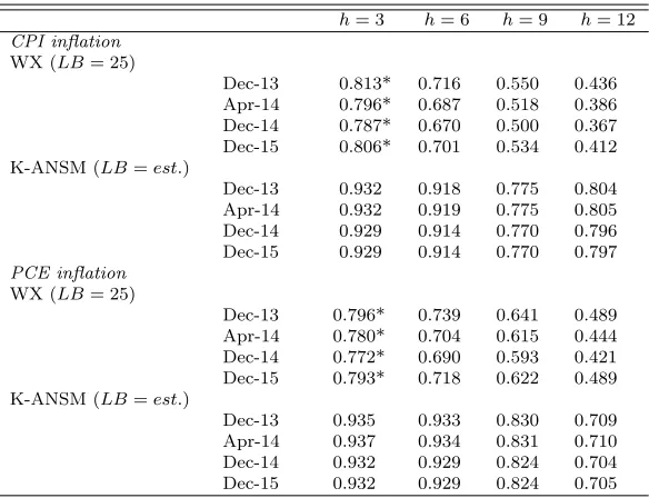
Table 8: Relative out-of-sample MSFE values for the ZLB period (re-estimated shadow rates)
h= 3 h= 6 h= 9 h= 12
CPI inflation
WX (LB= 25)
Dec-13 0.813* 0.716 0.550 0.436 Apr-14 0.796* 0.687 0.518 0.386 Dec-14 0.787* 0.670 0.500 0.367 Dec-15 0.806* 0.701 0.534 0.412 K-ANSM (LB=est.)
Dec-13 0.932 0.918 0.775 0.804 Apr-14 0.932 0.919 0.775 0.805 Dec-14 0.929 0.914 0.770 0.796 Dec-15 0.929 0.914 0.770 0.797
PCE inflation
WX (LB= 25)
Dec-13 0.796* 0.739 0.641 0.489 Apr-14 0.780* 0.704 0.615 0.444 Dec-14 0.772* 0.690 0.593 0.421 Dec-15 0.793* 0.718 0.622 0.489 K-ANSM (LB=est.)
Dec-13 0.935 0.933 0.830 0.709 Apr-14 0.937 0.934 0.831 0.710 Dec-14 0.932 0.929 0.824 0.704 Dec-15 0.932 0.929 0.824 0.705
Notes: The out-of-sample forecasting period runs from 2009:M1 to 2015:M12. Each row reports the ratio of the MSFE of the shadow rate forecasting model relative to the MSFE of the benchmark model. Asterisks mark rejection of the one-sided Diebold and Mariano (1995) test with the small sample modification by Harvey et al. (1997) at the 1% (***), 5% (**), and 10% (*) significance levels, respectively.
The results in Table 7 also show that the choice of the LB parameter does not
have a large effect on the forecasting performance of the shadow rates. The relative
MSFE values for the WX shadow rate are quite similar for all four LB parameters
considered in this study. Interestingly, the LB parameter seems to be somewhat more
important for the predictive power of the K-ANSM shadow rate. Consistent with the
in-sample results and the results in Table 5, the WX shadow rate with the LB parameter
of 14 bps outperforms the alternatives, whereas the K-ANSM shadow rate with the
LB parameter of 0 bps generates the best forecasts. These findings are intriguing.
The previous literature emphasizes that the LB parameter has a critical influence on
the shadow rate estimates. The sensitivity of the shadow rate estimates to the LB
parameter has been discussed, inter alia, in Christensen and Rudebusch (2015), Bauer
and Rudebusch (2016), and Krippner (2015a,b). This literature has shown that the
hand, the K-ANSM shadow rates have been found to be relatively robust. We conclude
from the evidence in Table 7 that when the purpose is to forecast future inflation, the
choice of the LB parameter does not matter much for the forecast accuracy of the
shadow rates.
As a sensitivity check, we repeat the above analysis using shadow rates estimated
with alternative sample periods. We consider the WX shadow rate with the LB
pa-rameter of 25 bps and the K-ANSM shadow rate with the estimated LB papa-rameter
(LB = 16), given their prevalent use in the extant literature. By comparing the
fore-casting performance of the shadow rates estimated with different data samples, we are
able to study whether the results in Table 7 are dependent on the specific data period
used in the estimation of the shadow rates. We think that this is a highly relevant
exercise. Krippner (2015a) demonstrates that the WX shadow rates re-estimated with
updated samples have different profiles over time. In contrast, he shows that the
K-ANSM shadow rate estimates are not sensitive to the choice of data sample used in
the estimation (cf. Figure 1).
The results of this sensitivity analysis, reported in Table 8, reveal that the
esti-mation sample does not matter much for the predictive power of the shadow rates.
Both the WX and K-ANSM shadow rates contain incremental predictive information
in the ZLB period regardless of which data sample is used in the estimation of the
shadow rates. In fact, the K-ANSM shadow rates perform almost identically in the
forecasting exercise. As one might expect based on the discussion in Krippner (2015a),
the choice of the estimation sample is more important for the WX shadow rate. Still,
the differences in the predictive ability are relatively small. The WX shadow rates
estimated with different data samples are very successful at predicting inflation in the
ZLB period, and they all dominate the best K-ANSM shadow rate.
We proceed by analyzing whether the model augmented with a shadow rate
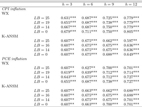
Table 9: Qualitative differences in predictive ability over the ZLB period
h= 3 h= 6 h= 9 h= 12
CPI inflation
WX
LB= 25 0.631*** 0.687*** 0.725*** 0.779***
LB= 19 0.655*** 0.687*** 0.738*** 0.779***
LB= 14 0.667*** 0.687*** 0.750*** 0.779***
LB= 0 0.679*** 0.711*** 0.750*** 0.805*** K-ANSM
LB= 25 0.607** 0.675*** 0.662*** 0.597**
LB= 16 0.607** 0.675*** 0.675*** 0.636***
LB= 14 0.607** 0.675*** 0.675*** 0.636***
LB= 0 0.607** 0.675*** 0.688*** 0.649***
PCE inflation
WX
LB= 25 0.607** 0.627** 0.700*** 0.701***
LB= 19 0.619** 0.639*** 0.712*** 0.714***
LB= 14 0.643*** 0.675*** 0.712*** 0.727***
LB= 0 0.655*** 0.687*** 0.738*** 0.727*** K-ANSM
LB= 25 0.607** 0.663*** 0.662*** 0.688***
LB= 16 0.607** 0.675*** 0.675*** 0.688***
LB= 14 0.607** 0.675*** 0.675*** 0.701***
LB= 0 0.607** 0.663*** 0.700*** 0.701***
Notes: The out-of-sample forecasting period runs from 2009:M1 to 2015:M12. Each row reports the fraction of observations for which the shadow rate forecast-ing model produces more accurate out-of-sample forecasts than the benchmark model. Asterisks mark rejection of the Diebold and Mariano (1995) sign test at the 1%(***), 5%(**), and 10%(*) significance levels, respectively.
of observations for which the model with a candidate shadow rate generates a smaller
absolute forecast error than the benchmark model. We test the statistical significance
using the Diebold and Mariano (1995) sign test. The results imply that the forecasts
from the models including a shadow rate are qualitatively superior to those from the
benchmark models. The shadow rate forecasting models provide more accurate
fore-casts for more than 50% of the observations for all dependent variable/forecast horizon
combinations. The differences in the forecasting accuracy are statistically significant.
This finding provides further evidence supporting the view that the WX and K-ANSM
shadow rates contain predictive power for U.S. inflation in the ZLB period when the
predictive information encoded in a large set of macroeconomic variables is already
taken into account. The WX shadow rates typically perform a bit better than the
K-ANSM shadow rates when we quantify out-of-sample forecast accuracy with a
Table 10: Out-of-sample performance of the WX versus the K-ANSM shadow rates
h= 3 h= 6 h= 9 h= 12
CPI inflation
Non-ZLB
LB= 25 0.997 0.986 0.959 0.947
LB= 16 0.997 0.986 0.959 0.948
LB= 14 0.997 0.986 0.959 0.948
LB= 0 0.996 0.989 0.960 0.949 ZLB
LB= 25 0.841*** 0.768** 0.685** 0.522**
LB= 16 0.856*** 0.788** 0.710** 0.558**
LB= 14 0.860*** 0.793** 0.715** 0.565**
LB= 0 0.890*** 0.825** 0.756** 0.616**
PCE inflation
Non-ZLB
LB= 25 0.994 0.969 0.960** 0.927*
LB= 16 0.994 0.966 0.961** 0.927*
LB= 14 0.994 0.966 0.961** 0.927*
LB= 0 0.995 0.966 0.963** 0.928* ZLB
LB= 25 0.849** 0.759** 0.709** 0.513**
LB= 16 0.865** 0.777** 0.731** 0.534**
LB= 14 0.869** 0.782** 0.735** 0.539**
LB= 0 0.891** 0.804** 0.768** 0.572**
Notes: Each row reports the ratio of the MSFE of the shadow rate forecasting model augmented with the WX shadow rate (LB= 25) relative to the MSFE of the shadow rate forecasting model augmented with the K-ANSM shadow rates. Asterisks mark rejection of the one-sided Diebold and Mariano (1995) test with the small sample modification by Harvey et al. (1997) at the 1% (***), 5% (**), and 10% (*) significance levels, respectively. The forecasting periods are as defined before.
has only a relatively small effect on the predictive power of the shadow rates.23
As a final exercise, we formally compare the relative out-of-sample forecasting
per-formance of the WX and K-ANSM shadow rates in Table 10. To save space, we report
the ratio of the MSFE of the shadow rate forecasting model augmented with the WX
shadow rate (LB = 25) relative to the MSFE of a forecasting model augmented with
different K-ANSM shadow rates (LB = 0,14,16,25). The results for the other WX
shadow rate specifications, shadow rates estimated with different data samples, and
qualitative differences in out-of-sample performance yield very similar conclusions.
The results in Table 10 show that the WX shadow rate produces better
out-of-23
sample inflation forecasts than the K-ANSM shadow rates. The WX shadow rate
dominates the K-ANSM shadow rates in both periods irrespective of which forecast
horizon is considered. As one might expect, the differences in forecast accuracy are
modest in the non-ZLB period. However, in the ZLB period, the WX shadow rate
produces substantially more accurate forecasts than the K-ANSM shadow rates. The
differences in forecast accuracy are statistically significant in the ZLB period. These
results provide further evidence supporting the findings in H¨annik¨ainen (2017).
One possible explanation for the relative forecasting performance of the shadow
rates is related to the way they are estimated from the yield curve data. The K-ANSM
shadow rates are estimated from a two-factor model (level and slope), whereas the WX
shadow rates are estimated using a three-factor term structure model (level, slope,
and curvature). Although the two-factor model generates more robust shadow rate
estimates than the three-factor model, it fits the yield curve data less closely than the
three-factor model (Krippner 2015a). It is well known that the yield curve (especially
the level factor) contains information about future inflation (see, e.g., Diebold and
Rudebusch 2013). Therefore, the fact that the WX shadow rate term structure model
fits better to the yield curve data and thus contains more information than the
K-ANSM model could, at least in part, explain why the WX shadow rate produces better
inflation forecasts than the K-ANSM shadow rate.
5.
Conclusions
This paper examines whether the shadow interest rates contain predictive power for
U.S. inflation in a data-rich environment. We focus on the shadow rates discussed in
Wu and Xia (2016) and Krippner (2015b), given their prevalent use in the literature.
Our empirical analysis leads us to three main conclusions. First, the shadow rates
inflation when the predictive information encoded in macroeconomic factors extracted
from a large set of 133 macroeconomic variables is already taken into account. This
finding holds both in the non-ZLB and ZLB periods. The forecasting performance of
the shadow rates is particularly good in the ZLB period. Therefore, our results suggest
that the shadow rates provide a valuable source of information about future inflation
for forecasters, central bankers, and other policymakers when the short-term rates
are stuck at the ZLB. Second, the relationship between the shadow rates and future
inflation is positive; i.e., if the shadow rate decreases, future inflation tends to decrease.
This result stems probably from the forward-looking nature of monetary policy. The
relationship between the shadow rate and future inflation tends to be stronger in the
ZLB environment for the WX shadow rate; but for the K-ANSM shadow rate the
relationship remains similar in both periods. Third, the WX shadow rates are more
informative about future inflation than the K-ANSM shadow rates. The WX shadow
rates produce better in-sample and out-of-sample inflation forecasts than the K-ANSM
shadow rates both in the non-ZLB and ZLB periods.
Interestingly, we find that the choice of the LB parameter or the sample period used
in the estimation of the shadow rates do not matter much for the predictive power of
the shadow rates. The results reveal that both the WX and K-ANSM shadow rates are
useful leading indicators for inflation regardless of which LB parameter or data sample
is used in the estimation of the shadow rates.
Our results could be extended in several ways. We have examined the predictive
power of the shadow rates for U.S. inflation. Evidence from other countries (e.g.,
from the eurozone, Japan and the U.K.) may lead to a better understanding of the
indicator properties of the shadow rates. Furthermore, we consider only point forecasts
in our out-of-sample forecasting exercise. However, density forecasts contain more
information than point forecasts, because they summarize the information regarding
institutions are interested in density forecasts. It would be interesting to know whether
the models augmented with a shadow rate produce better density forecasts than the
References
Atkeson, A. & Ohanian, L. E. (2001). Are Phillips curves useful for forecasting infla-tion? Federal Reserve Bank of Minneapolis Quarterly Review, 25, 2–11.
Bauer, M. D. & Rudebusch, G. D. (2016). Monetary policy expectations at the zero lower bound.Journal of Money, Credit and Banking, 48, 1439–1465 .
Bernanke, B. S. & Boivin, J. (2003). Monetary policy in a data-rich environment.
Journal of Monetary Economics, 50, 525–546.
Bernanke, B. S., Reinhart, V. R. & Sack, B. P. (2004). Monetary policy alternatives at the zero bound: An empirical assessment. Brookings Papers on Economic Activity, 2:2004, 1–78.
Christensen, J. & Rudebusch, G. D. (2015). Estimating shadow-rate term structure models with near-zero yields.Journal of Financial Econometrics, 13, 226–259.
Chung, H., Laforte, J-P., Reifschneider, D. & Williams, J. C. (2012). Have we under-estimated the likelihood and severity of zero lower bound events? Journal of Money, Credit and Banking, 44, 47–82.
Clark, T. E. & McCracken, M. W. (2013). Advances in Forecast Evaluation. In G. Elliott, & A. Timmermann (Eds), Handbook of Economic Forecasting, vol. 2, North-Holland, Amsterdam. 1107–1201.
Clements, M. P. (2016). Real-time factor model forecasting and the effects of instability.
Computational Statistics and Data Analysis, 100, 661–675.
Diebold, F. X. & Mariano, R. S. (1995). Comparing predictive accuracy. Journal of Business and Economic Statistics, 13, 253–265.
Diebold, F. X. & Rudebusch, G. D. (2013). Yield curve modeling and forecasting. Princeton: Princeton University Press.
Faust, J. & Wright, J. H. (2013). Forecasting inflation. In G. Elliott, & A. Timmermann (Eds), Handbook of Economic Forecasting, vol. 2, North-Holland, Amsterdam. 2–56.
Groen, J. J., Paap, R. & Ravazzolo, F. (2013). Real-time inflation forecasting in a changing world.Journal of Business and Economic Statistics, 31, 29-44.
G¨urkaynak, R., Sack, B. & Wright, J. (2007). The U.S. Treasury yield curve: 1961 to the present. Journal of Monetary Economics, 54, 2291–2304.
Harvey, D., Leybourne, S. & Newbold, P. (1997). Testing the equality of prediction mean squared errors.International Journal of Forecasting, 13, 281–291.
Kim, D. & Singleton, K. (2012). Term structure models at the zero bound: an empirical investigation of Japanese yields.Journal of Econometrics, 170, 32–49.
Krippner, L. (2015a). A comment on Wu and Xia (2015), and the case for two-factor shadow short rates. Australian National University CAMA Working Paper 48/2015, Australian National University.
Krippner, L. (2015b). Zero lower bound term structure modeling: A practitioner’s guide. NY: Palgrave-Macmillian.
Mishkin, F. S. (2017). Rethinking monetary policy after the crisis.Journal of Interna-tional Money and Finance, forthcoming.
McCracken, M. W. & Ng, S. (2016). FRED-MD: A Monthly Database for Macroeco-nomic Research.Journal of Business and Economic Statistics, 34, 574–589.
Neely, C. J. (2015). Unconventional monetary policy had large international effects.
Journal of Banking and Finance, 52, 101–111.
Nelson, C. & Siegel, A. (1987). Parsimonious modelling of yield curves. Journal of Business, 60, 473–489.
Newey, W. K. & West, K. D. (1987). A simple, positive semidefinite, heteroskedasticity and autocorrelation consistent covariance matrix. Econometrica, 55, 703–708.
Rossi, B. (2013). Advances in forecasting under instability. In G. Elliott, & A. Timmer-mann (Eds), Handbook of Economic Forecasting, vol. 2, North-Holland, Amsterdam. 1203–1324.
Sims, C. A. (1992). Interpreting the macroeconomic time series facts: The effects of monetary policy.European Economic Review, 36, 975–1000.
Stock, J. H. & Watson, M. W. (2002a). Forecasting using principal components from a large number of predictors. Journal of the American Statistical Association, 97, 1167– 1179.
Stock, J. H. & Watson, M. W. (2002b). Macroeconomic forecasting using diffusion indexes. Journal of Business and Economic Statistics, 20, 147–162.
Stock, J. H. & Watson, M. W. (2003). Forecasting output and inflation: The role of asset prices.Journal of Economic Literature, 41, 788–829.
Stock, J. H. & Watson, M. W. (2007). Why has U.S. inflation become harder to fore-cast? Journal of Money, Credit and Banking, 39, 3–33.
Stock, J. H. & Watson, M. W. (2016). Factor models and structural vector autoregres-sions in macroeconomics. In J. B. Taylor & H. Uhlig (Eds.) Handbook of Macroeco-nomics, vol. 2, North Holland, Amsterdam. 415–525.
Appendix A
Table A1: Data description
id Mnemonic Trans. code Description
1 RPI 5 Real Personal Income
2 W875RX1 5 Real Personal Income ex transfer receipts 3 DPCERA3M086SBEA 5 Real Personal Consumption Expenditures 4 CMRMTSPLx 5 Real Manu. and Trade Industries Sales 5 RETAILx 5 Retail and Food Services Sales
6 INDPRO 5 IP Index
7 IPFPNSS 5 IP: Final Products and Nonindustrial Supplies 8 IPFINAL 5 IP: Final Products (Market Group)
9 IPCONGD 5 IP: Consumer Goods 10 IPDCONGD 5 IP: Durable Consumer Goods 11 IPNCONGD 5 IP: Nondurable Consumer Goods 12 IPBUSEQ 5 IP: Business Equipment
13 IPMAT 5 IP: Materials 14 IPDMAT 5 IP: Durable Materials 15 IPNMAT 5 IP: Nondurable Materials 16 IPMANSICS 5 IP: Manufacturing (SIC) 17 IPB51222s 5 IP: Residential Utilities 18 IPFUELS 5 IP: Fuels
19 NAPMPI 1 ISM Manufacturing: Production Index 20 CUMFNS 2 Capacity Utilization: Manufacturing 21 HWI 2 Help-Wanted Index for United States 22 HWIURATIO 2 Ratio of Help Wanted/No. Unemployed 23 CLF16OV 5 Civilian Labor Force
24 CE16OV 5 Civilian Employment 25 UNRATE 2 Civilian Unemployment Rate
26 UEMPMEAN 2 Average Duration of Unemployment (Weeks) 27 UEMPLT5 5 Civilians Unemployed - Less Than 5 Weeks 28 UEMP5TO14 5 Civilians Unemployed for 5-14 Weeks 29 UEMP15OV 5 Civilians Unemployed - 15 Weeks & Over 30 UEMP15T26 5 Civilians Unemployed for 15-26 Weeks 31 UEMP27OV 5 Civilians Unemployed for 27 Weeks and Over 32 CLAIMSx 5 Initial Claims
33 PAYEMS 5 All Employees: Total nonfarm
34 USGOOD 5 All Employees: Goods-Producing Industries 35 CES1021000001 5 All Employees: Mining and Logging: Mining 36 USCONS 5 All Employees: Construction
37 MANEMP 5 All Employees: Manufacturing 38 DMANEMP 5 All Employees: Durable Goods 39 NDMANEMP 5 All Employees: Nondurable Goods
40 SRVPRD 5 All Employees: Service-Providing Industries 41 USTPU 5 All Employees: Trade, Transportation & Utilities 42 USWTRADE 5 All Employees: Wholesale Trade
43 USTRADE 5 All Employees: Retail Trade 44 USFIRE 5 All Employees: Financial Activities 45 USGOVT 5 All Employees: Government
46 CES0600000007 1 Avg Weekly Hours: Goods-Producing 47 AWOTMAN 2 Avg Weekly Overtime Hours: Manufacturing 48 AWHMAN 1 Avg Weekly Hours: Manufacturing
49 NAPMEI 1 ISM Manufacturing: Employment Index 50 HOUST 4 Housing Starts: Total New Privately Owned 51 HOUSTNE 4 Housing Starts, Northeast
52 HOUSTMW 4 Housing Starts, Midwest 53 HOUSTS 4 Housing Starts, South 54 HOUSTW 4 Housing Starts, West
55 PERMIT 4 New Private Housing Permits (SAAR)
56 PERMITNE 4 New Private Housing Premits, Northeast (SAAR) 57 PERMITMW 4 New Private Housing Permits, Midwest (SAAR) 58 PERMITS 4 New Private Housing Permits, South (SAAR) 59 PERMITW 4 New Private Housing Permits, West (SAAR) 60 NAPM 1 ISM: PMI Composite Index
Table A1 –(Continued)
id Mnemonic Trans. code Description
61 NAPMNOI 1 ISM: New Orders Index 62 NAPMSDI 1 ISM: Supplier Deliveries Index 63 NAPMII 1 ISM: Inventories Index 65 AMDMNOx 5 New Orders for Durable Goods
66 ANDENOx 5 New Orders for Nondefense Capital Goods 67 AMDMUOx 5 Unfilled Orders for Durable Goods 68 BUSINVx 5 Total Business Inventories
69 ISRATIOx 2 Total Business: Inventories to Sales Ratio
70 M1SL 6 M1 Money Stock
71 M2SL 6 M2 Money Stock
72 M2REAL 5 Real M2 Money Stock
73 AMBSL 6 St. Louis Adjusted Monetary Base 74 TOTRESNS 6 Total Reserves of Depository Institutions 75 NONBORRES 7 Reserves of Depository Institutions, Nonborrowed 76 BUSLOANS 6 Commercial and Industrial Loans, All Commercial Banks 77 REALLN 6 Real Estate Loans at All Commercial Banks
78 NONREVSL 6 Total Nonrevolving Credit Owner and Securitized Outstanding 79 CONSPI 2 Nonrevolving Consumer Credit to Personal Income
80 S & P 500 5 S&P’s Common Stock Price Index: Composite 81 S & P: indust 5 S&P’s Common Stock Price Index: Industrials 82 S & P div yield 2 S&P’s Composite Common Stock: Dividend Yield 83 S & P PE ratio 5 S&P’s Composite Common Stock: Price-Earnings Ratio 84 FEDFUNDS 2 Effective Federal Funds Rate
85 CP3Mx 2 3-Month AA Financial Commercial Paper Rate 86 TB3MS 2 3-Month Treasury Bill
87 TB6MS 2 6-Month Treasury Bill 88 GS1 2 1-Year Treasury Rate 89 GS5 2 5-Year Treasury Rate 90 GS10 2 10-Year Treasury Rate
91 AAA 2 Moody’s Seasoned Aaa Corporate Bond Yield 92 BAA 2 Moody’s Seasoned Baa Corporate Bond Yield 93 COMPAPFFx 1 3-Month Commercial Paper Minus FEDFUNDS 94 TB3SMFFM 1 3-Month Treasury C Minus FEDFUNDS 95 TB6SMFFM 1 6-Month Treasury C Minus FEDFUNDS 96 T1YFFM 1 1-Year Treasury C Minus FEDFUNDS 97 T5YFFM 1 5-Year Treasury C Minus FEDFUNDS 98 T10YFFM 1 10-Year Treasury C Minus FEDFUNDS
99 AAAFFM 1 Moody’s Aaa Corporate Bond Minus FEDFUNDS 100 BAAFFM 1 Moody’s Baa Corporate Bond Minus FEDFUNDS 101 TWEXMMTH 5 Trade Weighted U.S. Dollar Index: Major Currencies 102 EXSZUSx 5 Switzerland / U.S. Foreign Exchange Rate
103 EXJPUSx 5 Japan / U.S. Foreign Exchange Rate 104 EXUSUKx 5 U.S. / U.K. Foreign Exchange Rate 105 EXCAUSx 5 Canada / U.S. Foreign Exchange Rate 106 PPIFGS 6 PPI: Finished Goods
107 PPIFCG 6 PPI: Finished Consumer Goods 108 PPIITM 6 PPI: Intermediate Materials 109 PPICRM 6 PPI: Crude Materials
110 OILPRICEx 6 Crude Oil, spliced WTI and Cushing 111 PPICMM 6 PPI: Metals and Metal Products 112 NAPMPRI 1 ISM Manufacturing: Prices Index 113 CPIAUCSL 6 CPI: All Items
114 CPIAPPSL 6 CPI: Apparel 115 CPITRNSL 6 CPI: Transportation 116 CPIMEDSL 6 CPI: Medical Care 117 CUSR0000SAC 6 CPI: Commodities 118 CUUR0000SAD 6 CPI: Durables 119 CUSR0000SAS 6 CPI: Services
120 CPIULFSL 6 CPI: All Items Less Food 121 CUUR0000SA0L2 6 CPI: All Items Less Shelter 122 CUSR0000SA0L5 6 CPI: All Items Less Medical Care
123 PCEPI 6 Personal Cons. Expend.: Chain Price Index 124 DDURRG3M086SBEA 6 Personal Cons. Expend.: Durable Goods 125 DNDGRG3M086SBEA 6 Personal Cons. Expend.: Nondurable Goods 126 DSERRG3M086SBEA 6 Personal Cons. Expend.: Services
Table A1 –(Continued)
id Mnemonic Trans. code Description
127 CES0600000008 6 Avg Hourly Earnings: Goods-Producing 128 CES2000000008 6 Avg Hourly Earnings: Construction 129 CES3000000008 6 Avg Hourly Earnings: Manufacturing 130 UMCSENTx 2 Consumer Sentiment Index
131 MZMSL 6 MZM Money Stock
132 DTCOLNVHFNM 6 Consumer Motor Vehicle Loans Outstanding 133 DTCTHFNM 6 Total Consumer Loans and Leases Outstanding 134 INVEST 6 Securities in Bank Credit at All Commercial Banks
Figure A1: Factors over time
Time
f1
1985 1995 2005 2015
−25
−20
−15
−10
−5
0
5
Time
f2
1985 1995 2005 2015
−10
−5
0
5
Time
f3
1985 1995 2005 2015
−15
−10
−5
0
5
10
15
Time
f4
1985 1995 2005 2015
−6
−4
−2
0
2
4
6