Greenhouse Gases: A Review of Losses and Benefits

Munich Personal RePEc Archive

Greenhouse Gases: A Review of Losses

and Benefits

Ali, Amjad and Audi, Marc

Lahore School of Accountancy and Finance, University of Lahore

City Campus, Faculty of Business Administration, AOU

University/University Paris 1 Pantheon Sorbonne

2019

Online at

https://mpra.ub.uni-muenchen.de/96081/

1 | P a g e

Greenhouse Gases: A Review of Losses and Benefits

Amjad Ali

Lahore School of Accountancy and Finance, University of Lahore City Campus.

Marc Audi

Faculty of Business Administration, AOU University/University Paris 1 Pantheon Sorbonne.

Abstract

This study provides a review of benefit and losses of greenhouse gases. For the last decades, the average global temperature is rising on the surface as well as on the oceans. There are a number of factors behind this rise, but the main cause of this rise is anthropogenic increase in greenhouse gases (GHG). The anthropogenic factors comprise of burning of fossil fuel, coal mining, industrialization etc. During the last century, the CO2 concentration increased by 391 PPM, CH4 and N2O have reached at warming levels. The rise in overall temperature is changing the living pattern of humans and it also damages the economy as well as ecosystem for other living species. The rising GHG concentration may also have some positive effects on the economy, but it has heavy costs as well. GHGs are responsible for the change in climate which include a rise in sea level, ice melting from ice sheets and ocean acidification and climate change is responsible for the other damages like low fresh water resources, damage to the coastal system, damage to human health and raise the issue of food security.

Keywords: Greenhouse gases, health, food, natural resources

JEL Codes: N5, Q5

1. Introduction

The greenhouse gases are the important part of our ecosystem. Without the existence of Green House Gases (GHGs) our earth temperature would not be sustained. Instead of the importance of GHGs, the recent rise of GHGs is causing many damages to the human and other living beings. GHGs include CO2, CH4, N2O and CFC. Among them, the main contributor of global warming is CO2 [1], which is a long living gas in the atmosphere, before 200 years back it has reasonable level in the air. But due to industrialization, its amount reached to dangerous levels. Due to the high level of GHGs the average earth temperature is rising [2]. The hot and summer days are increasing throughout the earth and cool days and nights are diminishing. This hot summer adds to sea levels to more rise. In the snowy areas, the snow sheet is melting, which decreasing the reflectivity of the earth and increasing its energy absorption capacity. This increasing level of GHGs has very negative effects on human and animal’s health as well. The fresh water resources are also continuously decreasing and making the climate warmer. Although, there are

many empirical studies which highlights the dangerous impacts of GHG’s but GHGs have some advantages and benefits for the society. The CO2 is essential for the plants to grow, so increasing its concentration will give benefits to the plants also in some areas where precipitation increasing will have positive effects on the crops as well. But most of the scientific bodies are still agreeing that GHGs cost lot in terms of dry land loss and food security. Anthropogenic has become the main source of GHG’s concentration. The human activities which use the burning of fossil fuel, the raise the concentration level of CO2 in the atmosphere. Many empirical studies established direct relationship between economic growth and GHGs concentration, with rising population, day by day it is becoming difficult to forgo economic growth for the environment. The industrial countries like the USA and China are causing more damage to the environment as compared to the low-income countries. If the same trend of CO2 will continue till the end of the 21st century, there would be the high social cost of carbon human will face. The GHGs and its damage follow the pattern where GHGs, increases the temperature of the earth, which cause several damages to the planet. Scientific bodies are searching new technologies to mitigate the damages of GHGs.

2 | P a g e

1.1 Green House Gases

Our atmosphere is composed of several gases with different atmospheric concentration including Oxygen (21%), Nitrogen (78%), Water Vapor (0-4%), Argon (1%), Carbon Dioxide (0.04%), and others are Nitrous Oxide (trace), Methane (trace), Halo-carbon (trace) and Ozone (trace). These gases play a major role to make our earth's climate, sustainable for living beings. We inhale Oxygen when we breath. The trace gases have to maintain the temperature of our earth through a process called “greenhouse effect”. These trace gases are very low in quantity, but has very high impact on overall temperature. If these gases would not present in the atmosphere our atmosphere would be 30C cooler than the present temperature. There are three major components which define the greenhouse effects;

a) The heat absorbing capacity of that gas b) The atmospheric concentration of that gas c) The lifetime of that gas

According to the Donat et al., [3], the heat absorbing capacity of CH4 is 25 times greater than the CO2 and N20 has 296 times greater than C02. CO2 alone live more than 100 years in the atmosphere.

1.2 Logic Behind Green House Effect

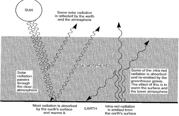
The Sun is the main source of energy in our solar system. It is impossible to live without the Sun. Energy from the Sun is due to the fusion process in which two atoms of hydrogen combine together and make a single atom of helium. In all this process, some of the hydrogen mass converted into energy. The Sun radiate energy in many ways (e. g light, heat, ultraviolet) and in the form of short waves (which contain huge amounts of energy). This energy reaches to the surface of the earth but before that our atmosphere which consist of gases stops 2/3 of the radiation from reaching to the earth. The remaining 1/3 reaches of the earth and some of its portion absorbed by the earth in the form of invisible radiation, after that our earth radiates this energy back towards space. All this process is called radiative forcing. The greenhouse gases stop the earth’s reflected energy going back to space and send back to earth. This whole process is called the greenhouse effect. The Oxygen and Nitrogen do not have any greenhouse effect. The most important GHG is CO2, which is only 0.04 of the atmospheres; it is clear that if the GHGs concentration will increase in the atmosphere they will stop more and more energy from going back to space and make earth warmer and warmer.

Figure 1: Illustration of Green House Effect

3 | P a g e

1.3. Concentration and Sources of GHGs

Many trace gases like CO2, N2O lives naturally in the atmosphere, but during recent days, it has been observed that concentrations of these gases is increasing in the atmosphere. The main cause of this concentration, is due to increase in anthropogenic, human activities like burning of fossil fuel etc.

1.3.1. Carbon Dioxide

It is a long-lived gas, the pre-industrial concentration of CO2 was 280 PPM [4], but today its concentration increased by 400 PPM. There are two major sources of this increase (I) burning of fossil fuel and (II) deforestation. This increase is enough to participate in greenhouse effect [5,6].

1.3.2. Methane

The second greenhouse gas is Methane CH4, the pre-industrial concentration of CH4 was 0.8 PPM [7,8]. In year 1978, the concentration was approx 1.51 PPM [9] and in the year 1990, the concentration was 1.71 PPM [10]. The recent concentration is 1890 PPB. The major source of CH4 is Natural Wetlands [11], Rice Paddie [12], Biomass burning [13], Coal Mine Ventilation [14], Leak from pipelines and discharge from oil and gas wells [14].

Figure 2: Carbon dioxide concentration since last 800000 years (left hand side) and since 1950 (right hand side)

Source: Environmental Protection agency

Figure 3: Methane concentration since last 800000 years (left hand side) and since 1950 (right hand side)

4 | P a g e

1.3.3. Nitrous Oxide

The Nitrous oxide is also one of the major components of the greenhouse effect. The pre-industrial concentration of N20 was 285 PPB [10] but in the year 1990, its concentration was 310 PPB [15] and in recent times, the concentration is increased by 328 PPB. The major source of N20 are Oceans [16], Aerobic Soil [17], and Fertilizers [18].

Figure 4: Nitrous oxide concentration since last 800000 years (left hand side) and since 1950 (right hand side)

Source: Environmental Protection agency

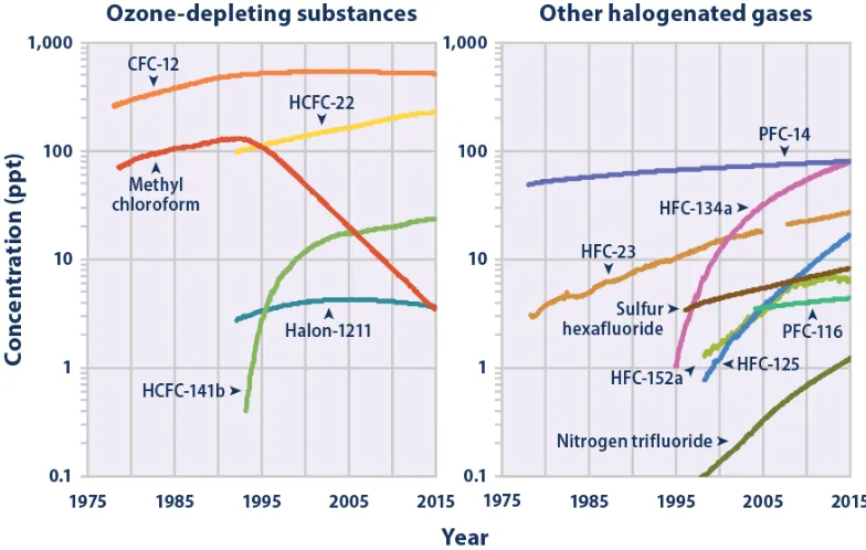
1.3.4. Halo-carbon

The other dominant source of the greenhouse effect is Halo-carbon, it includes CFC and HFC. It is mainly a product of industry and before industrialization, its concentration was almost zero and after industrialization different type of halo-carbons have different concentration. The halo-carbon are the most common cause of Ozone depletion [19].

1.3.5. Water Vapor

Another major player in the global warming scenario is water vapor. Increased water vapor in the atmosphere causes second atmospheric layer to cool and first layer of warmth [20,21,22]. But the concentration of water vapor is not affected by human activities. Since the pre-industrial time, many developed countries are sending CO2 emission in the air. The most concentration is sent from China after than USA. For more details view figure 6.

1.4. How Do We Know?

Almost all the scientific communities are agreed on the greenhouse effect, but there are uncertainties in the rate of change in radiative forcing due to changes in concentration. Statistical methods do not show any correlation between concentration and radiative forcing. To understand, the relationship between concentration and radiative forcing, we use radiative transfer models because our atmosphere is a very complex system. It is not only present value which affects the atmosphere, but also the past and future and the presence of cloudiness, water vapor also affects the atmosphere. The following equation is used to estimate the radiative forcing on the basis of change in concentration.

AF = f (C0, C) (1)

5 | P a g e

Figure 5: Halo Carbon concentration since 1975

Source: Environmental Protection agency

Figure 6: Global countries releasing CO2 in the atmosphere

Source: Environmental Protection agency

6 | P a g e

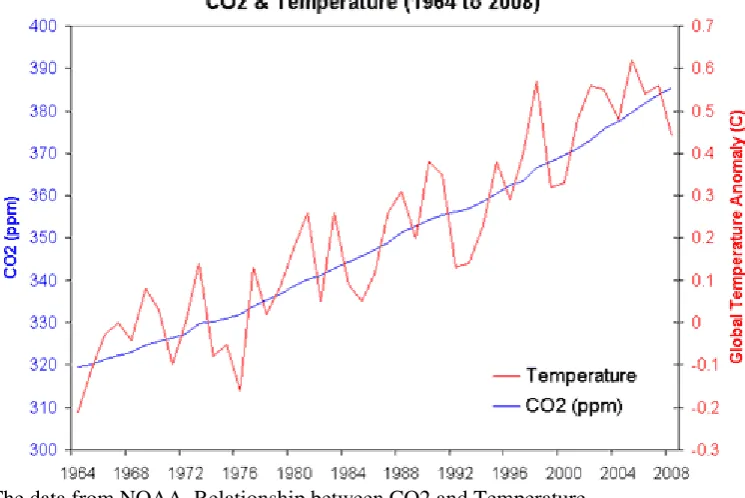
Followed by his work most of the studies has been conducted to find the relationship between GHGs and Global warming. Recently, we have evidence which suggest that the GHGs concentration is increasing since industrialization began which is causing global warming [26,27,28]. Global Warming is due to the increasing concentration of GHGs in the atmosphere [2,29,30]. The most known contributors of radiative forcing are CO2 (61%), CH4 (17%), N2O (4%) and CFCs (12%) [1]. CO2 is one of the major gas, which is causing a rise in the earth temperature [31]. Greenhouse gas concentration is causing Global warming, which is not only affecting land, but also the oceans at the same time [32]. IPCC in its AR4 concludes that in the troposphere, the concentration of GHGs is increasing and earth temperature is also increasing which is a clear sign that the global warming is related to the increased concentration of GHGs. Lacis et al., [33]

at NASA’s Goddard Institute for Space Studies (GISS) studied that Carbon Dioxide act like a thermostat

and control the earth temperature. There is not only the observed concentration of GHGs, but also the observed changes in the climate, like rise in sea level, ice sheets melting and change in precipitation which suggest that the earth is warming.

Figure 7: Statistical Method of finding the relationship between GHGs and Temperature shows that there is no correlation between these two variables. The CO2 continues to rise, but there is a variation in the temperature.

Source: The data from NOAA. Relationship between CO2 and Temperature.

2.Observed changes in Climate due to GHGs.

Plenty of changes have been observed in the climate due to increase in GHGs. The main change is in temperature as it is observed that the average temperature is rising all over the world. There is also change in Ice sheets and rising sea level.

2.1. Change in Temperature

2.1.1. Land Surface Air Temperature

IPCC AR4 mentioned that the Land Surface Air temperature is continuing to increase. GISS [34], GHCN [35], CRUTEM4 [36] and Berkeley [37] estimation of temperature concludes that since the year 1900 the earth temperature has risen. There are plenty of regional analysis has been conducted, including Europe [20,38,39,40], China [41,42,43,44], India [45], Australia [46], Canada [47], South America [48] and East Africa [49]. They all agree with the fact that the Earth Temperature is continuing to rise. As Antarctic is the coolest place in the world, but according to recent researches and data analysis [50, 51,52,53], they all are agreed that the Antarctic has been getting warmer since year 1950. The earth temperature has risen since 20th _{century had started and the warming is accelerating since year 1970. The NOAA data suggest}

7 | P a g e

the recorded history. There is a huge evidence that since about the year 1950, the global land areas faced warming in both max and min temperature extreme [3].

Figure 8: Global annual land surface air temperature anomalies. From 1961 to 1990 taken as an average

Source: Berkeley, CRUTEM, GHCN and GISS

2.1.2. Sea Surface Temperature

The Sea surface temperature is also continuously rising as overall GHGs concentration is rising. The results of four series such as ERSST [54, 55], HadSST2 [56], HadNMAT2 [57] suggest that the sea surface temperature is rising. The Satellite SST data records also suggest that there is a rapid increase in the sea surface temperature. Since the year 1880, there is almost 1.5C increase in the sea temperature and from year 1980, the increase is almost 1C. As time passes, the increase in the sea surface temperature is accelerating. The NOAA data suggest that since 2000 the SST has been increasing more sharply and the year 2016 was the warmest year in the recorded history.

Figure 9: Global annual land surface air temperature anomalies from 1880 to 2016

8 | P a g e

Table 1: Top 10 warmest years since 1880

Source: NOAA

Figure 10: Global annual sea surface temperature anomalies from 1859 to 2005

Source: HadSST2, HadSST3, ICOADS, HadNMAT2 RANK

1 = WARMEST

PERIOD OF RECORD: 1880–2016

YEAR ANOMALY °C ANOMALY °F

1 2016 0.94 1.69

2 2015 0.90 1.62

3 2014 0.74 1.33

4 2010 0.70 1.26

5 2013 0.67 1.21

6 2005 0.66 1.19

7 2009 0.64 1.15

8 1998 0.63 1.13

9 2012 0.62 1.12

10 (tie) 2003 0.61 1.10

10 (tie) 2006 0.61 1.10

9 | P a g e

2.2. Precipitation

It has been observed that the global trends in precipitation from 1901 to 2005 are statistically not good [58,59]. Since the year 1950, the extreme events like rainfall and droughts are worst [60]. These changes are attributed to global warming [61,62]. The change in global and regional precipitation is due to the anthropogenic forcing [63]. It has also been observed that there are shorter snowfall seasons and snow melting seasons start before the historical time [64]. In China, around 37% of the land facing drought with low soil moisture. Over the past century the global precipitation is decreasing CRU [65] and GHCN [19], the gauge-based precipitation data sets reveal that there has been a decrease in the precipitation globally from 1900 to 2005. In the USA, there is a change in the snowfall and in the western USA, the snowfall is converting into rain [66,67]. In the South Western part of Canada, the snowfall is decreasing [67]. In the heavy snow fall area of Japan, the snowfall is decreasing [19]. The snowfall and rainfall days in Switzerland also changed [68]. Monaghan and Bromwich [69] found a decline in the snowfall of the Antarctic in the year 2004. The decrease in the stream flow has been reported in mid and low latitude river basin like Yellow River since 1960 (Piao et al., 2010) where precipitation has been decreased. In some areas such as Part of USA the stream flow has been increased [70]. Analysis explain that there is a decrease in the cloud cover in may region of the world, including Poland [71], China and Tibetan Plateau [72,73,74], particular the clouds at the upper level [75] and also over Africa, South America and Eurasia and in particular [75]. Although the satellite measurement shows that the heavy rainfall during the warmest years [76].

Figure 11: Global annual sea surface temperature anomalies from 1880 to 2016

Source: NOAA

2.3. Sea Level Rise

During the 18th _{century, the European ports installed the tide gauges to measure the sea level. Since then}

10 | P a g e

the atmosphere, the temperature is tending to rise, which is causing the effect of thermal expansion in the sea and increasing ocean heat content. In the recent times, the tide gauges record is available to check the sea level. The record suggests that sea level is rising over the 20th _{century [79,80]. The rate of change in}

the sea level from 1901 to 2010 was 1.7 mm/yr. During the year 2017, the measurements show that the average sea level increase is 84.8 mm since 1993 and from the year 1870 the total change is almost 190 mm. The sea level is continually increasing at a rate of 1/8 of an inch per year. The data suggest that there is an upward trend in the sea level change. Although, it is difficult to find the exact value of sea level change due to global warming because there are other factors like vertical land changes also affect the sea level but using satellite and updated tide gauge technology a comprehensive record on sea level rise with the correction of vertical land changes.

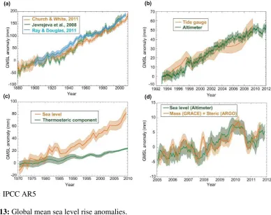
Figure 12: Global mean sea level rise anomalies

Source: IPCC AR5

Figure 13: Global mean sea level rise anomalies.

11 | P a g e

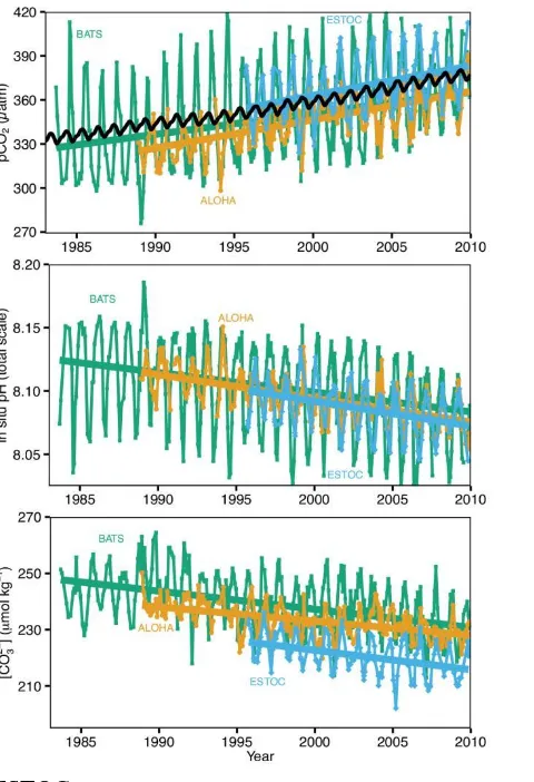
2.4. Ocean Acidification

Oceans are the main reservoir of CO2. Ocean store 50 times more CO2 as compared to the atmosphere [81]. So, the oceans are the important sink for CO2. According to [82,83] 30% of total anthropogenic emission is stored by the oceans. The oceans uptake CO2 and make a weak acid H2CO3. The approx oceans PH is almost between 7.8 to 8.4 which is greater than 7, so oceans do not have any acid component in it. The recent trend shows that there is a decrease in the oceans PH which is causing the ocean acidification [84]. The global decrease in surface PH of the oceans was 0.08 from 1765 to 1994[81]. The CO2 is the dominant cause of the change in oceanic chemistry [85]. Although Oceans do a lot to uptake the extra CO2 from the atmosphere, but it is causing rise in the oceans as well. There is plenty of damage for ocean life as well. If anthropogenic CO2 will increase at this amount by the end of the year 2100, the oceans PH will reduce to 7.4 which is a very dangerous sign for human and sea life at the same time.

2.5. Changes in Cryosphere

Cryosphere is referred to the water in the frozen state. It has several components, including snow, river ice shelves, and lake ice, ice sheets, sea ice, ice caps and glaciers. Ice on the surface is very necessary for earth albedo because of its 95% reflectivity. Arctic is a sea which is covered with ice almost whole the year. Its ice extent varies seasonally about in the summer 6 × 106 km2 and in winter about 15 × 106 km2 [86,87]. In recent observation, it is observed that Arctic Ice sheet losing its mass. The mass loss occurs in summer more rapidly as compare to winter [87,89]. In 2012 the ice extent was 3.44 × 106 km2 and in 2007 the extent was 4.22 × 106 km2 [89]. The Arctic is losing its area and also the thickness of the ice sheet [90].

Figure 14: The time series data of Atlantic and North Pacific oceans, which show pCO2 (top), pH (center) and Carbonate ion (bottom)

12 | P a g e

Figure 15: Ice area and Ice extent of Central Arctic from 1979 to 2012

Source: Comiso [88]

13 | P a g e

Figure 16: Different Ice measurement of Arctic sea ice including ALMS, SIDS and MYIA

14 | P a g e

Table 2

Period Ice sheet loss (mm yr–1 SLE) Greenland

2005–2010 (6-year)

0.63 ±0.17

1993–2010 (18-year)

0.33 ±0.08

Antarctica

2005–2010 (6-year)

0.41 ±0.20

1993–2010 (18-year)

0.27 ±0.11

Combined

2005–2010 (6-year)

1.04 ±0.37

1993–2010 (18-year)

0.60 ±0.18

Source: IPCC AR5

The Greenland temperature has risen since 1990s [104]. On the regional level, many studies have been conducted and they conclude that ice in lakes and rivers is continuing to fall [105,106]. The permafrost temperature is continuing to rise [55, 107]. The rise in permafrost temperature release CO2 in the atmosphere which again causing increases in the CO2 [108,109,110]. Since 1980, the temperature has risen by 2C. There is a decreasing trend in the discharge of the top 200 rivers, including the Congo, Yenisei, Mississippi, Parana, Columbia, Ganges, Niger and Uruguay, since 1948 to 2004 [111]

Figure 17: The Ice mass loss equivalent to sea level from the Greenland and Antarctica

Source: IPCC AR5

3. Impact on Human Life 3.1 Fresh Water Resources

15 | P a g e

to fall. Due to climate change the snow in many areas is converting into rain and those areas which rely on snow in the dry season will not be able to extract the benefit of snow in the form of fresh water and they face severe drought. Glaciers melting can also cause flooding and destroy the crops where there are no proper measures are taken to avoid floods. Water is used to produce energy with low amount of water and lack of stream-flow and river discharge will affect the production of electricity as well, which will in another case shift this production to more coal and oil usage which will again cause global warming. The more CO2 and energy production with sources other than water will pollute more and more fresh water resources. Due to the heavy rainfall which is observed in some area the soil erosion is another issue.

3.2 Coastal system

There are three major things which are affecting the marine coastal system; Sea Level Rise, Ocean Warming, Ocean Acidification. Due to the ocean acidification the ocean water is turning into the weak acid, which is reducing the calcium in the oceans, it is causing lots of problems for sea animals like coral reef or shell fish. Due to the oceans warming most of the species migrating towards the cold water. The ocean is changing the habitat of the marine species. The sea level rise has plenty of problems for humans. Due to the sea level rise most of the ocean’s shoreline are shifting their path which is decreasing the dry land. Erosion is another problem which is due to sea level rise. Rising sea level will drown some plants and animals as well. Warmer temperature causes oral bleaching which weaken some animals and they face high mortality rate. Due to the warmer temperature and the sea level rise there are high chances of floods and storms which will cause damage to the society. Oceans warming will cause species to die as almost 17% of our food come from the sea and almost 3 billion people consume protein from the sea. Almost 90% of the transportation of goods and services are from the oceans due to the climate change, so all these things will be affected by the sea. Almost 40% of our population live in cities where the land meets the sea. Due to the Sea level rise most of our population will expose to the sea. In the year 2010 almost 270 million people are exposed to the sea.

3.3 Human Health

As temperature warm up, the heat related deaths have increased. In the tropical region of the world heat related deaths significantly increase in the past decade. According to the WHO, each year 12.6 million deaths are happening because of the climate. There are three ways by which climate effect the lifestyle; First direct effect, which include extreme weather, heat, drought etc. Second, effects through natural system which include diseases and pollution. Third, effects through human system which include mental stress, under nutrition etc. There is a direct relationship between hot days increase and increase in mortality [115]. IPCC in its special report SREX concludes that there is a decrease in cold days and increase in the hot days and it is very likely that heat related deaths will also increase [116]. In the year 2012, there are almost 15000 deaths happened in France alone due to heat [117]. Human body temperature is almost 38C and if the outside temperature increase by 40.6C, there is a high chance of organ damage and loss of consciousness [118]. Due to the climate change, the floods will happen and in the year 2011, 6 out of 10 biggest disasters were flooding the total number of people died were 3140 [119]. Flooding and windstorms affect human health by drowning, infectious diseases (e.g. vector borne disease, injuries and cholera [120,121]. In countries, where warm days are increasing vector borne diseases are also increasing like malaria, dengue fever etc. Most commonly, the climate change is destroying the ozone layer which will cause the sun UV rays to pass through it and it can cause skin cancer and skin burn. The estimate of deaths related to forest fires was 339,000 deaths per year, and from 260,000 to 600,000 deaths are related to air pollution [122].

3.4 Food Security

16 | P a g e

moisture, which is causing a negative effect on the food production. Decrease in the food production, causing increases in the food security. The major crops like wheat, rice and maize are fully impacted by the increase in the temperature. It is causing damage to these crops as rice needs a lot of water to grow, but due to temperature rise the water is evaporating quickly, which is causing a decrease in the production also premature growth of crops is also observed. Due to warming the crop insects are increasing and the damage due to these insects is almost 16 to 18% [125]. The other remaining plants are treated by a lot of protests which is decreasing the quality of crops.

Figure 18: Price index

Source: IPCC AR5

4. Benefits of GHGs

17 | P a g e

Figure 19: Rice yield change, Wheat yield change, Maize yield change in terms of temperature change

Source: IPCC AR5

5. Conclusions

Green House Gases are dangerous for the future of the human and other living beings lives on the planet. Although, many measures are taken to mitigate the severeness of GHGs, but yet they are causing harm to human life. Currently, the increasing concentration of GHGs is creating difficulties for human beings to live on the planet. If these GHGs are not controlled properly, it can make our earth warmer enough to end life on the planet. Many disadvantages are still hidden, but scientific body is working to find and predict the changes in the planet's atmosphere due to the GHGs. In some cases, the confidence and evidence are low, but yet the evidence we were enough to predict that our future on this planet is at risk. Mitigating GHGs concentration is not easy and belong to a single country or governments of the countries, but every individual has to play its key role to overcome bad outcomes of economic growth. Although there are many claims which shows the benefits of GHGs, but these benefits are in the short run in the long run the GHGs are damaging the earth.

References

18 | P a g e

[2] Lashof DA. The dynamic greenhouse: feedback processes that may influence future concentrations of atmospheric trace gases and climatic change. Climatic change 1989;1;14(3):213-42.

[3] Donat MG, Alexander LV, Yang H, Durre I, Vose R, Dunn RJ, Willett KM, Aguilar E, Brunet M, Caesar J, Hewitson B. Updated analyses of temperature and precipitation extreme indices since the beginning of the twentieth century: The HadEX2 dataset. Journal of Geophysical Research: Atmospheres 2013;118(5):2098-118.

[4] Neftel A, Moor E, Oeschger H, Stauffer B. Evidence from polar ice cores for the increase in atmospheric CO2 in the past two centuries. Nature 1985;315(6014):45-47.

[5] Hansen J, Lacis A, Rind D, Russell G, Stone P, Fung I, Ruedy R, Lerner J. Climate sensitivity: Analysis of feedback mechanisms. Climate processes and climate sensitivity 1984;1:130-63. [6] Broccoli AJ, Manabe S. The influence of continental ice, atmospheric CO 2, and land albedo on

the climate of the last glacial maximum. Climate dynamics 1987;1(2):87-99.

[7] Craig H, Chou CC. Methane: The record in polar ice cores. Geophysical Research Letters 1982;9(11):1221-4.

[8] Khalil MA, Rasmussen RA. Carbon monoxide in the earth's atmosphere: increasing trend. Science 1984;224(4644):54-56.

[9] Blake DR, Rowland FS. Continuing worldwide increase in tropospheric methane, 1978 to 1987. Science 1988;239(4844):1129-31.

[10] Zander R, Demoulin P, Ehhalt DH, Schmidt U. Secular increase of the vertical column abundance of methane derived from IR solar spectra recorded at the Jungfraujoch station. Journal of Geophysical Research: Atmospheres 1989;94(D8):11029-39.

[11] Svensson BH, Rosswall T. In situ methane production from acid peat in plant communities with different moisture regimes in a subarctic mire. Oikos 1984;341-50.

[12] Aselmann I, Crutzen PJ. Global distribution of natural freshwater wetlands and rice paddies, their net primary productivity, seasonality and possible methane emissions. Journal of Atmospheric chemistry 1989;8(4):307-58.

[13] Crutzen PJ, Delany AC, Greenberg J, Haagenson P, Heidt L, Lueb R, Pollock W, Seiler W, Wartburg A, Zimmerman P. Tropospheric chemical composition measurements in Brazil during the dry season. Journal of Atmospheric Chemistry 1985;2(3):233-56.

[14] Cicerone RJ, Oremland RS. Biogeochemical aspects of atmospheric methane. Global biogeochemical cycles 1988;2(4):299-327.

[15] Elkins JW, Rossen R. Summary Report 1988: Geophysical monitoring for climatic change. NOAA ERL, Boulder, CO. 1989.

[16] McElroy MB, Wofsy SC. Tropical forests: Interactions with the atmosphere, Tropical Rain Forests and the World Atmosphere. GT Prance 1986:33-60.

[17] Matson PA, Vitousek PM. Cross‐system comparisons of soil nitrogen transformations and nitrous oxide flux in tropical forest ecosystems. Global Biogeochemical Cycles 1987;1(2):163-70. [18] Bremner JM, Breitenbeck GA, Blackmer AM. Effect of nitrapyrin on emission of nitrous oxide

from soil fertilized with anhydrous ammonia. Geophysical Research Letters. 1981;8(4):353-6. [19] Vose RS, Schmoyer RL, Steurer PM, Peterson TC, Heim R, Karl TR, Eischeid JK. The Global

Historical Climatology Network: Long-term monthly temperature, precipitation, sea level pressure, and station pressure data. Oak Ridge National Lab., TN (United States). Carbon Dioxide Information Analysis Center; 1992.

[20] Böhm R, Jones PD, Hiebl J, Frank D, Brunetti M, Maugeri M. The early instrumental warm-bias: a solution for long central European temperature series 1760–2007. Climatic Change 2010;101(1-2):41-67.

[21] Manabe S, Strickler RF. Thermal equilibrium of the atmosphere with a convective adjustment. Journal of the Atmospheric Sciences 1964;21(4):361-85.

19 | P a g e

[23] Hansen J, Fung I, Lacis A, Rind D, Lebedeff S, Ruedy R, Russell G, Stone P. Global climate changes as forecast by Goddard Institute for Space Studies three‐dimensional model. Journal of geophysical research: Atmospheres 1988;93(D8):9341-64.

[24] Wigley TM, Raper SC. Thermal expansion of sea water associated with global warming. Nature 1987;330(6144):127.

[25] Arrhenius S. XXXI. On the influence of carbonic acid in the air upon the temperature of the ground. The London, Edinburgh, and Dublin Philosophical Magazine and Journal of Science 1896;41(251):237-76.

[26] Hurtt GC, Chini LP, Frolking S, Betts RA, Feddema J, Fischer G, Goldewijk KK, Hibbard K, Janetos A, Jones CD, Kindermann G. Harmonisation of global land-use scenarios for the period 1500–2100 for IPCC-AR5. 2009.

[27] Oreskes N. The scientific consensus on climate change. Science 2004;306(5702):1686.

[28] Keeling CD, Bacastow RB, Carter AF, Piper SC, Whorf TP, Heimann M, Mook WG, Roeloffzen H. A three‐dimensional model of atmospheric CO2 transport based on observed winds: 1. Analysis of observational data. Aspects of climate variability in the Pacific and the Western Americas 1989:165-236.

[29] Kelly PM, Wigley TM. The influence of solar forcing trends on global mean temperature since 1861. Nature 1990;347(6292):460.

[30] Gregory J, Stouffer RJ, Molina M, Chidthaisong A, Solomon S, Raga G, Friedlingstein P, Bindoff NL, Le Treut H, Rusticucci M, Lohmann U. Climate change 2007: the physical science basis 2007. [31] Hansen J, Johnson D, Lacis A, Lebedeff S, Lee P, Rind D, Russell G. Climate impact of increasing

atmospheric carbon dioxide. Science 1981;213(4511):957-66.

[32] Willis JK, Chambers DP, Kuo CY, Shum CK. Global sea level rise: Recent progress and challenges for the decade to come. Oceanography 2010;23(4):26-35.

[33] Lacis AA, Schmidt GA, Rind D, Ruedy RA. Atmospheric CO2: Principal control knob governing

Earth’s temperature. Science 2010;330(6002):356-9.

[34] Hansen J, Ruedy R, Sato M, Lo K. Global surface temperature change. Reviews of Geophysics 2010;48(4).

[35] Lawrimore JH, Menne MJ, Gleason BE, Williams CN, Wuertz DB, Vose RS, Rennie J. An overview of the Global Historical Climatology Network monthly mean temperature data set, version 3. Journal of Geophysical Research: Atmospheres 2011;116(D19).

[36] Morice CP, Kennedy JJ, Rayner NA, Jones PD. Quantifying uncertainties in global and regional temperature change using an ensemble of observational estimates: The HadCRUT4 data set. Journal of Geophysical Research: Atmospheres 2012;27:117(D8).

[37] Rohde R, Muller RA, Jacobsen R, Muller E, Perlmutter S, Rosenfeld A, Wurtele J, Groom D, Wickham C. A new estimate of the average Earth surface land temperature spanning 1753 to 2011. Geoinfor Geostat Overview 2013;7:2.

[38] Winkler P. Revision and necessary correction of the long-term temperature series of Hohenpeissenberg, 1781–2006. Theoretical and applied climatology 2009;98(3-4):259-68. [39] Tietäväinen H, Tuomenvirta H, Venäläinen A. Annual and seasonal mean temperatures in Finland

during the last 160 years based on gridded temperature data. International Journal of Climatology 2010;30(15):2247-56.

[40] Schrier G, Ulden AV, Van Oldenborgh GJ. The construction of a Central Netherlands temperature. Climate of the Past 2011;7(2):527-42.

[41] Li Q, Zhang H, Liu X, Chen J, Li W, Jones P. A mainland China homogenized historical temperature dataset of 1951–2004. Bulletin of the American Meteorological Society 2009;90(8):1062-5.

[42] Zhen L, Zhong-Wei Y. Homogenized daily mean/maximum/minimum temperature series for China from 1960-2008. Atmospheric and Oceanic Science Letters 2009;2(4):237-43.

20 | P a g e

[44] Tang G, Ding Y, Wang S, Ren G, Liu H, Zhang L. Comparative analysis of China surface air temperature series for the past 100 years. Advances in Climate Change Research. 2010;1(1):11-19.

[45] Jain SK, Kumar V. Trend analysis of rainfall and temperature data for India. Current Science(Bangalore) 2012;102(1):37-49.

[46] Trewin B. A daily homogenized temperature data set for Australia. International Journal of Climatology 2013;33(6):1510-29.

[47] Vincent LA, Wang XL, Milewska EJ, Wan H, Yang F, Swail V. A second generation of homogenized Canadian monthly surface air temperature for climate trend analysis. Journal of Geophysical Research: Atmospheres 2012;117(D18).

[48] Falvey M, Garreaud RD. Regional cooling in a warming world: Recent temperature trends in the southeast Pacific and along the west coast of subtropical South America (1979–2006). Journal of Geophysical Research: Atmospheres 2009;114(D4).

[49] Christy JR, Norris WB, McNider RT. Surface temperature variations in East Africa and possible causes. Journal of Climate 2009;22(12):3342-56.

[50] O’Donnell R, Lewis N, McIntyre S, Condon J. Improved methods for PCA-based reconstructions: Case study using the Steig et al.(2009) Antarctic temperature reconstruction. Journal of Climate 2011;24(8):2099-115.

[51] Chapman WL, Walsh JE. A synthesis of Antarctic temperatures. Journal of Climate. 2007;20(16):4096-117.

[52] Steig EJ, Schneider DP, Rutherford SD, Mann ME, Comiso JC, Shindell DT. Warming of the Antarctic ice-sheet surface since the 1957 International Geophysical Year. Nature 2009;457(7228):459.

[53] Monaghan AJ, Bromwich DH, Chapman W, Comiso JC. Recent variability and trends of Antarctic near‐surface temperature. Journal of Geophysical Research: Atmospheres 2008;113(D4).

[54] Smith TM, Peterson TC, Lawrimore JH, Reynolds RW. New surface temperature analyses for climate monitoring. Geophysical Research Letters 2005;32(14).

[55] Smith TM, Reynolds RW, Peterson TC, Lawrimore J. Improvements to NOAA’s historical merged land–ocean surface temperature analysis (1880–2006). Journal of Climate 2008;21(10):2283-96.

[56] Rayner NA, Brohan P, Parker DE, Folland CK, Kennedy JJ, Vanicek M, Ansell TJ, Tett SF. Improved analyses of changes and uncertainties in sea surface temperature measured in situ since the mid-nineteenth century: The HadSST2 dataset. Journal of Climate 2006;19(3):446-69. [57] Kent EC, Rayner NA, Berry DI, Saunby M, Moat BI, Kennedy JJ, Parker DE. Global analysis of

night marine air temperature and its uncertainty since 1880: The HadNMAT2 data set. Journal of Geophysical Research: Atmospheres 2013;118(3):1281-98.

[58] Schulte-Uebbing L, Hansen G, Hernandez AM, Winter M. Chapter scientists in the IPCC AR5— experience and lessons learned. Current opinion in environmental sustainability 2015;14:250-6. [59] Bates B, Kundzewicz Z, Wu S. Climate change and water. Intergovernmental Panel on Climate

Change Secretariat; 2008.

[60] Arndt DS, Baringer MO, Johnson MR. State of the climate in 2009. Bulletin of the American Meteorological Society 2010;91(7):s1-222.

[61] Stott PA, Gillett NP, Hegerl GC, Karoly DJ, Stone DA, Zhang X, Zwiers F. Detection and attribution of climate change: a regional perspective. Wiley Interdisciplinary Reviews: Climate Change 2010;1(2):192-211.

[62] Lambert O, Piroux M, Puyo S, Thorin C, Larhantec M, Delbac F, Pouliquen H. Bees, honey and pollen as sentinels for lead environmental contamination. Environmental Pollution 2012;170:254-9.

[63] Zhang X, Zwiers FW, Hegerl GC, Lambert FH, Gillett NP, Solomon S, Stott PA, Nozawa T. Detection of human influence on twentieth-century precipitation trends. Nature 2007;448(7152):461.

21 | P a g e

of space-borne radiometer data and ground-based measurements. Remote Sensing of Environment 2011;115(12):3517-29.

[65] Mitchell TD, Jones PD. An improved method of constructing a database of monthly climate observations and associated high‐resolution grids. International journal of climatology 2005;25(6):693-712.

[66] Feng S, Hu Q. Changes in winter snowfall/precipitation ratio in the contiguous United States. Journal of Geophysical Research: Atmospheres 2007;112(D15).

[67] Kunkel KE, Palecki MA, Ensor L, Easterling D, Hubbard KG, Robinson D, Redmond K. Trends in twentieth-century US extreme snowfall seasons. Journal of Climate 2009;22(23):6204-16. [68] Serquet G, Marty C, Dulex JP, Rebetez M. Seasonal trends and temperature dependence of the

snowfall/precipitation‐day ratio in Switzerland. Geophysical research letters 2011;38(7); L07703. [69] Monaghan AJ, Bromwich DH. Advances in describing recent Antarctic climate variability.

Bulletin of the American Meteorological Society 2008;89(9):1295-306.

[70] Groisman PY, Knight RW, Karl TR, Easterling DR, Sun B, Lawrimore JH. Contemporary changes of the hydrological cycle over the contiguous United States: Trends derived from in situ observations. Journal of hydrometeorology 2004;5(1):64-85.

[71] Wibig J. Cloudiness variations in Łódź in the second half of the 20th century. international Journal of climatology 2008;28(4):479-91.

[72] Duan A, Wu G. Change of cloud amount and the climate warming on the Tibetan Plateau. Geophysical Research Letters 2006;33(22), L22704.

[73] Endo N, Yasunari T. Changes in low cloudiness over China between 1971 and 1996. Journal of climate 2006;19(7):1204-13.

[74] Xia X. Spatiotemporal changes in sunshine duration and cloud amount as well as their relationship in China during 1954–2005. Journal of Geophysical Research: Atmospheres 2010;115(D7). [75] Warren SG, Eastman RM, Hahn CJ. A survey of changes in cloud cover and cloud types over land

from surface observations, 1971–96. Journal of Climate 2007;20(4):717-38.

[76] Allan RP, Soden BJ. Atmospheric warming and the amplification of precipitation extremes. Science 2008;321(5895):1481-84.

[77] Church JA, White NJ. Sea-level rise from the late 19th to the early 21st century. Surveys in geophysics 2011;32(4-5):585-602.

[78] Warrick RA, Oerlemans J. Sea level rise 1990.

[79] Mitchum GT, Nerem RS, Merrifield MA, Gehrels WR. Modern sea‐level‐change estimates. Understanding Sea‐Level Rise and Variability 2010:122-42.

[80] Woodworth PL, White NJ, Jevrejeva S, Holgate SJ, Church JA, Gehrels WR. Evidence for the accelerations of sea level on multi‐decade and century timescales. International Journal of Climatology: A Journal of the Royal Meteorological Society 2009;29(6):777-89.

[81] Sabine CL, Feely RA, Gruber N, Key RM, Lee K, Bullister JL, Wanninkhof R, Wong CS, Wallace DW, Tilbrook B, Millero FJ. The oceanic sink for anthropogenic CO2. Science 2004;305(5682):367-71.

[82] Le Quéré C, Takahashi T, Buitenhuis ET, Rödenbeck C, Sutherland SC. Impact of climate change and variability on the global oceanic sink of CO2. Global Biogeochemical Cycles 2010;24(4). [83] Mikaloff Fletcher SE, Gruber N, Jacobson AR, Doney SC, Dutkiewicz S, Gerber M, Follows M,

Joos F, Lindsay K, Menemenlis D, Mouchet A. Inverse estimates of anthropogenic CO2 uptake, transport, and storage by the ocean. Global Biogeochemical Cycles 2006;20(2).

[84] Keeling CD, Brix H, Gruber N. Seasonal and long‐term dynamics of the upper ocean carbon cycle at Station ALOHA near Hawaii. Global Biogeochemical Cycles 2004;18(4).

[85] Feely RA, Doney SC, Cooley SR. Ocean acidification: Present conditions and future changes in a high-CO₂ world. Oceanography 2009;22(4):36-47.

[86] Comiso JC, Nishio F. Trends in the sea ice cover using enhanced and compatible AMSR‐E, SSM/I, and SMMR data. Journal of Geophysical Research: Oceans 2008;113(C2).

[87] Cavalieri DJ, Parkinson CL. Arctic sea ice variability and trends, 1979-2010. The Cryosphere 2012;6(4):881.

22 | P a g e

[89] Comiso JC, Parkinson CL, Gersten R, Stock L. Accelerated decline in the Arctic sea ice cover. Geophysical research letters 2008;35(1).

[90] Wadhams P. Evidence for thinning of the Arctic ice cover north of Greenland. Nature 1990;345(6278):795.

[91] Zwally HJ, Comiso JC, Parkinson CL, Cavalieri DJ, Gloersen P. Variability of Antarctic sea ice 1979–1998. Journal of Geophysical Research: Oceans 2002;107(C5):9-1.

[92] Comiso JC, Kwok R, Martin S, Gordon AL. Variability and trends in sea ice extent and ice production in the Ross Sea. Journal of Geophysical Research: Oceans 2011;116(C4).

[93] Wadhams P, Tucker WB, Krabill WB, Swift RN, Comiso JC, Davis NR. Relationship between sea ice freeboard and draft in the Arctic Basin, and implications for ice thickness monitoring. Journal of Geophysical Research: Oceans 1992;97(C12):20325-34.

[94] Leclercq M, Mathieu O, Gomez E, Casellas C, Fenet H, Hillaire-Buys D. Presence and fate of carbamazepine, oxcarbazepine, and seven of their metabolites at wastewater treatment plants. Archives of environmental contamination and toxicology 2009;56(3):408.

[95] Gardner W, Olson DM. Population census of Megacopta cribraria (Hemiptera: Plataspidae) in kudzu in Georgia, USA, 2013–2016. Journal of Entomological Science 2016;51(4):325-8. [96] Rabatel A, Guérin C, Siouffi G, Sorlin S. Ethique, point (s) de vue et rapport aux différents régimes

de vérité. C. Guérin, G. Siouffi & S. Sorlin (éds), Le rapport éthique au discours 2013:65-80. [97] Rabassa J, Coronato A. Glaciations in Patagonia and Tierra del Fuego during the Ensenadan

Stage/Age (Early Pleistocene–earliest Middle Pleistocene). Quaternary International 2009;210(1-2):18-36.

[98] Bolch T, Kulkarni A, Kääb A, Huggel C, Paul F, Cogley JG, Frey H, Kargel JS, Fujita K, Scheel M, Bajracharya S. The state and fate of Himalayan glaciers. Science 2012;336(6079):310-4. [99] Olesen JE, Børgesen CD, Elsgaard L, Palosuo T, Rötter RP, Skjelvåg AO, Peltonen-Sainio P,

Börjesson T, Trnka M, Ewert F, Siebert S. Changes in time of sowing, flowering and maturity of cereals in Europe under climate change. Food Additives & Contaminants: Part A 2012;29(10):1527-42.

[100] Shepherd A, Ivins ER, Geruo A, Barletta VR, Bentley MJ, Bettadpur S, Briggs KH, Bromwich DH, Forsberg R, Galin N, Horwath M. A reconciled estimate of ice-sheet mass balance. Science 2012;338(6111):1183-9.

[101] Sasgen I, van den Broeke M, Bamber JL, Rignot E, Sørensen LS, Wouters B, Martinec Z, Velicogna I, Simonsen SB. Timing and origin of recent regional ice-mass loss in Greenland. Earth and Planetary Science Letters 2012;333:293-303.

[102] Ivins ER, Watkins MM, Yuan DN, Dietrich R, Casassa G, Rülke A. On‐land ice loss and glacial isostatic adjustment at the Drake Passage: 2003–2009. Journal of Geophysical Research: Solid Earth 2011;116(B2).

[103] Thomas ID, King MA, Bentley MJ, Whitehouse PL, Penna NT, Williams SD, Riva RE, Lavallee DA, Clarke PJ, King EC, Hindmarsh RC. Widespread low rates of Antarctic glacial isostatic adjustment revealed by GPS observations. Geophysical Research Letters 2011;38(22).

[104] Wang JM, Firestone MK, Beissinger SR. Microbial and environmental effects on avian egg viability: Do tropical mechanisms act in a temperate environment? Ecology 2011;92(5):1137-45. [105] Benson D, Jordan A, Cook H, Smith L. Collaborative environmental governance: are watershed

partnerships swimming or are they sinking? Land Use Policy 2013;30(1):748-57.

[106] Yu L, Wang G, Zhang R, Zhang L, Song Y, Wu B, Li X, An K, Chu J. Characterization and source apportionment of PM2. 5 in an urban environment in Beijing. Aerosol Air Qual. Res 2013;13(2):574-83.

[107] Lin YY, Chen CW, Chu TH, Su WF, Lin CC, Ku CH, Wu JJ, Chen CH. Nanostructured metal oxide/conjugated polymer hybrid solar cells by low temperature solution processes. Journal of Materials Chemistry 2007;17(43):4571-6.

23 | P a g e

[109] Zimov SA, Davydov SP, Zimova GM, Davydova AI, Schuur EA, Dutta K, Chapin III FS. Permafrost carbon: Stock and decomposability of a globally significant carbon pool. Geophysical Research Letters 2006;33(20).

[110] Qiao NA, Schaefer D, Blagodatskaya E, Zou X, Xu X, Kuzyakov Y. Labile carbon retention compensates for CO2 released by priming in forest soils. Global Change Biology 2014;20(6):1943-54.

[111] Dai DF, Rabinovitch PS. Cardiac aging in mice and humans: the role of mitochondrial oxidative stress. Trends in cardiovascular medicine 2009;19(7):213-20.

[112] Gerten D, Heinke J, Hoff H, Biemans H, Fader M, Waha K. Global water availability and requirements for future food production. Journal of hydrometeorology 2011;12(5):885-99. [113] Aguilera H, Murillo JM. The effect of possible climate change on natural groundwater recharge

based on a simple model: a study of four karstic aquifers in SE Spain. Environmental Geology 2009;57(5):963-74.

[114] Viviroli D, Archer DR, Buytaert W, Fowler HJ, Greenwood G, Hamlet AF, Huang Y, Koboltschnig G, Litaor I, López-Moreno JI, Lorentz S. Climate change and mountain water resources: overview and recommendations for research, management and policy. Hydrology and Earth System Sciences 2011;15(2):471-504.

[115] Lee H, Kim H, Honda Y, Lim YH, Yi S. Effect of Asian dust storms on daily mortality in seven metropolitan cities of Korea. Atmospheric environment 2013;79:510-7.

[116] Christidis N, Stott PA, Zwiers FW, Shiogama H, Nozawa T. The contribution of anthropogenic forcings to regional changes in temperature during the last decade. Climate Dynamics 2012;39(6):1259-74.

[117] Fouillet A, Rey G, Wagner V, Laaidi K, Empereur-Bissonnet P, Le Tertre A, Frayssinet P, Bessemoulin P, Laurent F, De Crouy-Chanel P, Jougla E. Has the impact of heat waves on mortality changed in France since the European heat wave of summer 2003? A study of the 2006 heat wave. International journal of Epidemiology 2008;37(2):309-17.

[118] Wyndham CH, Strydom NB. The danger of an inadequate water intake during marathon running. South African Medical Journal 1969;43(7).

[119] Guha-Sapir D, Vos F, Below R, Ponserre S. Annual disaster statistical review 2010. Centre for Research on the Epidemiology of Disasters 2011.

[120] Jakubicka T, Vos F, Phalkey R, Guha-Sapir D, Marx M. Health impacts of floods in Europe: data gaps and information needs from a spatial perspective. Centre for Research on the Epidemiology of Disasters (CRED); 2010.

[121] Raddatz TJ, Reick CH, Knorr W, Kattge J, Roeckner E, Schnur R, Schnitzler KG, Wetzel P, Jungclaus J. Will the tropical land biosphere dominate the climate–carbon cycle feedback during the twenty-first century? Climate Dynamics 2007;29(6):565-74.

[122] Reid CE, Brauer M, Johnston FH, Jerrett M, Balmes JR, Elliott CT. Critical review of health impacts of wildfire smoke exposure. Environmental Health Perspectives 2016;124(9):1334-43. [123] Lobell DB, Schlenker W, Costa-Roberts J. Climate trends and global crop production since 1980.

Science 2011;333(6042):616-20.

[124] Rivero RM, Mestre TC, Mittler RO, Rubio F, GARCIA‐SANCHEZ FR, Martinez V. The combined effect of salinity and heat reveals a specific physiological, biochemical and molecular response in tomato plants. Plant, cell & environment 2014;37(5):1059-73.

[125] Oerke EC. Crop losses to pests. The Journal of Agricultural Science 2006;144(1):31-43.

[126] Koo BH, Yoo SC, Park JW, Kwon CT, Lee BD, An G, Zhang Z, Li J, Li Z, Paek NC. Natural variation in OsPRR37 regulates heading date and contributes to rice cultivation at a wide range of latitudes. Molecular Plant 2013;6(6):1877-88.

[127] Jaggard KW, Qi A, Semenov MA. The impact of climate change on sugarbeet yield in the UK: 1976–2004. The Journal of Agricultural Science 2007;145(4):367-75.