Endogenous Dynamic Efficiency in the Intertemporal Optimization Models of Firm Behavior

Munich Personal RePEc Archive

Endogenous Dynamic Efficiency in the

Intertemporal Optimization Models of

Firm Behavior

Tsionas, Mike G. and Malikov, Emir and Kumbhakar, Subal

C.

Lancaster University Management School, University of Nevada, Las

Vegas, State University of New York at Binghamton

27 November 2019

Online at

https://mpra.ub.uni-muenchen.de/97780/

Endogenous Dynamic Efficiency in the Intertemporal

Optimization Models of Firm Behavior

∗

Mike G. Tsionas1 Emir Malikov2 Subal C. Kumbhakar3,4

1_{Lancaster University Management School, Lancaster, United Kingdom}

2

University of Nevada, Las Vegas, NV, United States

3

State University of New York at Binghamton, Binghamton, NY, United States

4

University of Stavanger Business School, Stavanger, Norway

November 27, 2019

Abstract

Existing methods for the measurement of technical efficiency in the dynamic production models obtain it from the implied distance functions without making use of the information about in-tertemporal economic behavior in the estimation beyond an indirect appeal to duality. The main limitation of such an estimation approach is that it does not allow for the dynamic evolution of efficiency that is explicitly optimized by the firm. This paper introduces a new conceptualiza-tion of efficiency that directly enters the firm’s intertemporal producconceptualiza-tion decisions and is both explicitly costly and endogenously determined. We build a moment-based multiple-equation system estimation procedure that incorporates both the dynamic and static optimality condi-tions derived from the firm’s intertemporal expected cost minimization. We operationalize our methodology using a modified version of a Bayesian Exponentially Tilted Empirical Likelihood adjusted for the presence of dynamic latent variables in the model, which we showcase using the 1960–2004 U.S. agricultural farm production data. We find that allowing for potential en-dogenous adjustments in efficiency over time produces significantly higher estimates of technical efficiency, which is likely due to inherent inability of the more standard exogenous-efficiency model to properly credit firms for incurring efficiency-improvement adjustment costs. Our re-sults also suggest material improvements in efficiency over time at an about 2.6% average annual rate, which contrasts with near-zero estimates of the exogenous efficiency change.

Keywords: dynamic efficiency, endogenous efficiency, intertemporal optimization, Bayesian analysis, Markov Chain Monte Carlo, sequential Monte Carlo

JEL Classification: C11, D24, Q10

∗_{Email: [email protected] (Tsionas), [email protected] (Malikov), [email protected]}

(Kumb-hakar).

1

Introduction

The use of explicit dynamic models of the firm’s intertemporal production decisions to account for and provide estimates of technical (in)efficiency are still relatively scarce in the efficiency analysis literature. Most existing studies rely on the static formulations of firm production (e.g., see Parme-ter & Kumbhakar, 2014; Kumbhakar, ParmeParme-ter & Zelenyuk, 2017, for recent surveys). However, for such static production models to provide a reasonably accurate description of the firm behavior, the firm ought to be able to freely adjust all its inputs at any point in time which would obviate any dynamic implications of its production decisions. In practice though, not all factors of production are freely-varying in the face of adjustment frictions (e.g., time-to-install, hiring costs) that may render them quasi-fixed in the short run. This notable weakness of the static production models (and hence of the static inefficiency measurements derived therefrom) owing to their inability to accommodate gradual adjustments in dynamic inputs, whereby the present production decisions have dynamic implications for future production outcomes, has recently given rise to a new strand of literature focused on incorporating intertemporal aspects of firm optimization into the efficiency measurement. The work of Silva & Stefanou (2003, 2007) is a fundamental advance on these is-sues, wherein the authors develop a dynamic optimization model of the firm production behavior using intertemporal cost minimization with quasi-fixed factors, based upon which they propose a nonparametric1 _{measure of dynamic (technical) efficiency (see Kapelko & Oude Lansink, 2017,}

for a multi-direction extension). Alternatively, Rungsuriyawiboon & Stefanou (2007) use a shadow cost approach in a similar intertemporal cost minimization framework to nonparametrically recover efficiency measures under dynamic duality. For some earlier but simpler attempts to nonparametri-cally model dynamic aspects of the firm production, also see Sengupta (1995) and Nemoto & Goto (1999, 2003). More recently, Serra, Oude Lansink & Stefanou (2011) and Silva & Oude Lansink (2013) have proposed a measurement of dynamic efficiency based on a primal directional-distance-function-based representation of production technology which has been gaining popularity in the literature partly because it can be operationalized via both the data envelopment and (econometric) stochastic frontier methods.2 _{This formulation has since been extended to enable a decomposition}

of dynamic efficiency (Kapelko, Oude Lansink & Stefanou, 2014) and to also measure “dynamic” productivity growth (Oude Lansink, Stefanou & Serra, 2015), with multiple empirical applications that have followed.

While the theoretical models of dynamic production decisions do explicitly postulate the firm’s intertemporal optimization subject to adjustment frictions in quasi-fixed inputs, available method-ologies for the estimation of dynamic efficiency in such frameworks in practice hardly make use of the information embedded in such dynamic optimization problems. Rather, the popular go-to approach

1

Estimated using the (non-stochastic) data envelopment analysis.

2

is to estimate technical efficiency from Silva & Oude Lansink’s (2013) dynamic directional distance function (oriented in the space of freely-varying inputs and investments into quasi-fixed dynamic factors) under its duality to the optimal current value function associated with the firm’s intertem-poral cost-minimization problem under the Hamilton-Jacobi-Bellman conditions (e.g., Serra et al., 2011; Kapelko et al., 2014; Oude Lansink et al., 2015; Kapelko, Oude Lansink & Stefanou, 2016, 2017; Minviel & Sipil¨ainen, 2018). Thus, in practice, the strategy for a (primal) estimation of dynamic technical efficiency is effectively the same as that for the estimation of a more conven-tional static efficiency except that in the former case a distance to the frontier is measured in the space of variable inputsand investments as opposed to merely conditioning the distance function on quasi-fixed levels of dynamic inputs. For instance, if one were to adopt econometric techniques, the estimation then boils down to a familiar procedure of appending a convoluted stochastic error containing a one-sided latent inefficiency and a two-sided noise to the distance function a pos-teriori. Such an estimation approach may however be overly restrictive because it (i) does not explicitly account for dynamics in efficiency itself as well as does not allow for the costly firm-controlled efficiency change, (ii) neglects the likely possibility that past dynamic efficiency is a part of the information set based upon which the firm optimizes, (iii) makes no use of information about economic behavior in the estimation beyond an indirect appeal to duality despite seeking a deeply structural “dynamic” interpretation of efficiency, and (iv) suffers from the endogeneity problem due to simultaneity of the variable input and investment decisions. Lastly and perhaps more importantly, the underlying conceptual framework of dynamic production that the available estimation methodologies are based upon does not allow for the dynamic evolution of efficiency that is explicitly optimized by the firm. While conditioning of the distance function on investments in dynamic inputs implicitly allows a departure from the strong assumption of exogenous efficiency by letting the firm to indirectly control the evolution of its efficiency (through investment decisions), such an endogenization of dynamic efficiency is derivative/indirect in its nature. It also implicitly assumes away the costliness of efficiency changes beyond the costs derived from frictions in dynamic inputs thereby dispensing with the expenses pertaining specifically to efficiency improvements such as adoption of quality control and other improved business practices, management training, etc.

Our methodology for the estimation of dynamic efficiency therefore provides a more elaborate alternative to that based on dynamic distance functions estimated under duality which restrictively treats efficiency as exogenous and distributed independently over time (e.g., see Serra et al., 2011). Now, ours is not the first attempt to explicitly model temporal dynamics of latent technical efficiency econometrically, where a few earlier works include Ahn, Good & Sickles (2000) and Tsionas (2006). However, to our knowledge, no prior study has done so in conjunction with a full intertemporal optimization problem of the firm like we do in this paper which, among other things, enables us to endogenize inefficiency as well as to explicitly accommodate its costliness in the firm optimization.3 The latter is particularly desirable given the interest of economists in linking dynamic efficiency to adjustment costs and the real option values of investment (e.g., Lambarraa, Stefanou & Gil, 2016). We showcase our model by applying it to an annual state-level panel data on agricultural farm production in lower 48 contiguous states of the United States during the 1960–2004 period. We follow Gallant, Giocomini & Ragusa (2017) to estimate models involving moment conditions and latent dynamic variables, although we do not use a Metropolis-Hastings approach or sequential importance sampling because Sequential Monte Carlo is more efficient. We use a modified version of a Bayesian Exponentially Tilted Empirical Likelihood adjusted for the presence of dynamic la-tent variables in the model (i.e., variable-inputs-oriented technical efficiency and quasi-fixed factor distortions) that, among other things, does not rely on using a fully parametric likelihood. The joint dynamics of latent variables is formulated using a second-order vector autoregression, with the choice of order motivated by temporal dynamics in the firm’s Euler equations. Among other things, we find that the failure to allow for potential endogenous adjustments in efficiency over time produces significantly lower estimates of dynamic efficiency, which is likely due to the in-herent inability of a more traditional exogenous-efficiency framework to properly credit producing units for incurring efficiency-improvement adjustment costs. The data overwhelmingly support our approach.

The rest of the paper proceeds as follows. Section 2 introduces our model of dynamic production decisions in the presence of endogenous efficiency. We describe the estimation details in Section 3. Section 4 reports the empirical application. We conclude in Section 5.

2

Model

Consider the dynamic production process. Let xt∈ ℜJ+ denote the vector of freely varying inputs

with wt ∈ ℜJ++ being the vector of corresponding prices. Further, let kt ∈ ℜM+ be the vector of

quasi-fixed dynamic factors of production andq_t∈ ℜM++denote their corresponding “rental” prices

(user costs). Bothwt andqtmay evolve stochastically over time. Suppose alsoδ= [δ1, . . . , δM]′ ∈

[0,1]M _{is a vector of depreciation rates, and β ∈ [0,1) is a time discount factor. The vector of}

outputs is given byy_t∈ ℜQ+.

In line with the tradition in the literature on dynamic efficiency, we consider an intertemporal

3

cost minimization but, unlike previous studies, incorporate inefficiency directly into the optimiza-tion problem as well as allow for uncertainty. The uncertainty, in this case, can arise from the lack of perfect foresight about future market conditions including the input prices that may evolve over time stochastically. We also assume firms are risk-neutral. The risk-neutrality assumption is made primarily so that, in the firm optimization problem under uncertainty, we can work directly with the expectation of a future stream of costs (the outcomes) without needing to consider the optimization of their expected utilities. In this choice, we have opted to follow the convention in the literature on costly investments into dynamic factors under uncertainty. More specifically, we build on the seminal work by Pindyck & Rotemberg (1983). While we recognize that risk-neutrality may be too restrictive of an assumption, the advantage of such a formulation is that it provide us with the tractable way of modeling the firm’s intertemporal behavior that gives rise to the Euler conditionsin expectation which we then use as a basis to form the estimating moment conditions. Notably, our setup is already more flexible than the existing work on dynamic efficiency that as-sumes that the forward-looking firms have perfect foresight (e.g., Silva & Stefanou, 2003, 2007; Rungsuriyawiboon & Stefanou, 2007; Serra et al., 2011; Silva & Oude Lansink, 2013).

Firms are said to operate in perfectly competitive factor markets rendering present and future input prices exogenous. To highlight key features of our modeling approach, we begin with a simpler standard framework with no inefficiency, which we then augment step by step to incorporate (i) explicitly costly and (ii) endogenously determined inefficiency.

Optimization without Inefficiency. The firm’s more traditional intertemporal expected cost optimization problem with respect to dynamic inputs is given by

min

k_t E0

∞

X

t=0

βt

   

C(wt,kt,yt) + M X

m=1 h

qm,tkm,t+Gm km,t−(1−δm)km,t−1

| {z }

im,t

i    

, (2.1)

where E0 denotes expectation at time t = 0 conditional on the available information; each mth

quasi-fixed dynamic input follows its respective law of motion, i.e.,

km,t =im,t+ (1−δm)km,t−1 ∀ m,

withim,t being the gross investment flow into this input’s stock;Gm(·) is the function representing

adjustment costs in km ∀ m; and C(w,k,y) : ℜJ++× ℜM+ × ℜQ+ → ℜ+ is the restricted

(short-run) variable cost function optimized in the freely-varying static factors subject to the already predetermined quasi-fixedk_t:

C(wt,kt,yt)≡min_x

t

w′_txt: F(xt,kt,yt) = 1, (2.2)

Optimization Subject to Exogenous Inefficiency. To introduce inefficiency, we begin by con-sidering the firm’s static optimization problem where we introduce a possibility for the over/under-use of inputs `a la Kumbhakar (1997), i.e.,

min

x_t w

′

txt: F(ϑtxt,ηt⊙kt,yt) = 1, (2.3)

with the scalarxt-oriented technical inefficiency ϑt≥1 measuring over-use in all freely varying

in-puts and each element ofη_t= [η1,t, . . . , ηM,t]′∈ ℜM++representing a distortion in the corresponding

quasi-fixed factor (i.e., the over- or under-use thereof). Note that, to capture likely heterogeneity in the degree of fixity acrosskt, the factor distortions {ηm,t} are permitted to vary across individual

quasi-fixed inputs. The above problem is equivalent to

Cw_t,ek,y_t≡min

e

x_t ϑ

−1

t w′txet: F

e

x_t,ek_t,y_t= 1, (2.4)

wherex_et≡ϑtxt and ekt≡ηt⊙kt are the actual input quantities; and it is evident that the firm’s

actual cost is Ca(w_t,ke_t,y_t) = ϑtC(wt,ekt,yt) and, hence, lnCa(wt,ekt,yt) = lnC(wt,ekt,yt) +

ut with ut ≡ lnϑt ∈ ℜ+ measuring variable cost inefficiency arising from the firm’s technical

inefficiency in thext orientation.

Thus, extending framework in (2.1)–(2.2) to explicitly allow for exogenous inefficiency and factor distortions taken by the firm as given, we obtain the following dynamic optimization problem:

min

e

k_t E0

∞

X

t=0

βt

(

ϑtC

wt,ekt,yt

+

M X

m=1 h

qm,tekm,t+Gm

e

km,t−(1−δm)ekm,t−1 i)

, (2.5)

with all endogenous choice variables measuring actual quantities employed in the production and, thus, the optimization objective being reflective of actual costs inclusive of inefficiencies.

Optimization with Endogenous Inefficiency. While already an improvement over the more traditional framework, the model in (2.4)–(2.5) continues to assume that inefficiency is effectively random and that the firm has no impact on the extent of variable input over-use in its produc-tion. Now, although oftentimes not stated explicitly, technical inefficiency in the stochastic frontier analysis is assumed to be known to a decision maker at the firm. However, it is rarely made clear whether inefficiency can be changed unless the model specification allows for the “environmental” factors determining it. This raises a few questions. If inefficiency is known to the decision maker, why is she not reducing it? Can inefficiency be freely adjusted or is this a costly adjustment process? What is the optimal inefficiency level, if any?

decisions. To endogenize dynamic efficiency, we therefore further generalize intertemporal expected cost minimization objective as follows:

min

e

k_t,ϑt E0

∞

X

t=0

βt

    ϑtC

w_t,ke_t,y_t+

M X

m=1 h

qm,tekm,t+Gm

e

km,t−(1−δm)ekm,t−1 i

+H lnϑt−lnϑt−1

| {z }

Vt

    ,

(2.6)

where H(·) is a function that captures adjustment costs in ϑt, i.e., the cost of improvements in

the xt-oriented dynamic efficiency; and the dynamic inefficiency evolves according to a controlled

log-linear law of motion:

lnϑt=Vt+ lnϑt−1,

with Vt being the improvement4 in inefficiency ϑt; and C(·) is as defined in (2.4). Thus, dynamic

inefficiency plays the role of an additional state variable. Here, we effectively conceptualize ϑt

akin to a dynamic intangible “input” subject to adjustment frictions that result in delayed changes therein. Analogously, Vt may be thought of as a “net investment” into improved efficiency. We

postulate the law of motion forϑt in logs to transform its codomain to have the evolving variable

be non-negative just like other dynamic state variables {km,t}.

A few more remarks about our conceptualization of inefficiency in the context of the firm’s dynamic production decisions. First, just like in the standard stochastic frontier analysis, we do not model inefficiency as a measure relative to other firms’ performance but as a deviation from the firm’s own “true frontier.” Thus, for the decision maker to know her firm’s inefficiency, no knowledge about other firms is required. Second, we assume that the decision maker knows the firm’s inefficiency, but the latter is unknown to the econometrician. This inefficiency comes from the firm’s failure to attain its production frontier. Such failures may be due to bad luck, machine breakdown, mismanagement, human errors, etc. If she does not know it exactly, the decision maker at the firm is reasonably expected at least to have a good estimate of such inefficiency. Third, production decisions and the efficiency are oftentimes influenced by exogenous contextual factors that the firm takes into consideration when optimizing and that are neither inputs nor outputs. We have abstracted away from such a possibility having instead opted for a simpler model in order to not distract the reader from the main focus of our paper which is on the endogenization of inefficiency. Empirically however, such contextual factors can be seamlessly accounted for by conditioning the variable cost function on them thereby effectively treating them as the “y” variables that, just like the output quantities, are exogenous and quasi-fixed under the cost-minimization premise.

Also, note that, for computational tractability of our econometric model, in (2.6) we continue to maintain the assumption that distortions in quasi-fixed factors {ηm,t} are exogenous to the

firm albeit, in principle, one can endogenize those as well. As it is to become clearer below, we

4

do nonetheless allow{ηm,t} to also be time-persistent thereby indirectly accommodating dynamic

properties therein.

The key feature of our model is that it treats technical inefficiency ϑt(the adjustments therein,

to be precise) as an additional “choice” variable which generates the optimal path ofϑtcompatible

with the firm’s intertemporal cost minimization, thereby enhancing its structurally meaningful interpretation. The optimization problem also implies that{ηm,t}, which impact the actual use of

quasi-fixed inputs{ekm,t}, cannot be independent over time.

The Euler equations corresponding to the problem in (2.6) are

0 = ϑt

∂C(·)

∂ekm,t

+qm,t+

∂Gm(·)

∂im,t −

β(1−δm)Et

∂Gm(·)

∂im,t+1

∀m= 1, . . . , M (2.7)

0 = ϑtC(·) +

∂H(·)

∂Vt

−βEt

H(·)

∂Vt+1

, (2.8)

along with the (actual) conditional demand equations for static inputs from (2.4):

xj,t =ϑt

∂C(·)

∂wj,t

∀ j= 1, . . . , J. (2.9)

Note that, in our setup, both the variable-input-oriented technical inefficiency ϑt and the

dis-tortions in quasi-fixed inputsη_t are the short-run measures because they affect the firm’s outputs in time t. Their long-run counterparts would be a solution to the system in (2.7)–(2.9) when all other variables are at their long-run stead-steady values.

For the practical implementation, we make the following parametric functional form assump-tions. The variable cost function is said to take the translog form, i.e.,

lnC(wt,ke,yt) =αo+αw′ lnwt+ 1₂lnw′tΓwwlnwt +

α′_k(lnkt+ξt) +12(lnkt+ξt)′Γkk(lnkt+ξt) + lnwt′Γwk(lnkt+ξt) +

α′_ylny_t+1₂lny′_tΓyylnyt+ lnyt′Γywlnwt+ lny′tΓyk(lnkt+ξt) + lnϑt (2.10)

≡C_{(lnwt,lnkt+ξ}

t,lnyt;θ) + lnϑt, (2.11)

where α0,αw,αk,αy and Γww,Γkk,Γwk,Γyy,Γyw,Γyk are respectively vectors and (symmetric)

matrices of conformable dimensions containing unknown parameters, which we denote collectively by θ∈ ℜP_{; and}

lnke= ln(η_t⊙kt) = lnkt+ξt,

with ξ_t ≡ lnη_t ∈ ℜM and lnϑt ∈ ℜ+ being, respectively, the unobservable quasi-fixed factor

distortion and inefficiency terms (in logs).

Pindyck & Rotemberg, 1983; Hall, 2004):

Gm(im,t) = 1₂γmim,t2 with γm>0, ∀ m= 1, . . . , M (2.12)

H(Vt) = 1₂γoVt2 with γo>0 (2.13)

and, for convenience, we letγ= [γ1, . . . , γM, γo]′.

With this, the system of dynamic and static optimizing conditions in (2.7)–(2.9) then takes the following form (maintaining the order of appearance of equations):

0 = ϑt

ηm,t h

α_k+Γ_kk(lnkt+ξt) +Γwklnwt+Γyklnyt

i_exp{C_{(lnwt,lnkt+ξ}

t,lnyt;θ)}

km,t

+

qm,t+γm

ηm,tkm,t−(1−δm)ηm,t−1km,t−1

−

γmβ(1−δm)Et n

ηm,t+1km,t+1−(1−δm)ηm,tkm,t o

∀ m= 1, . . . , M (2.14) 0 = ϑtexp{C(lnwt,lnkt+ξt,lnyt;θ)}+γo(lnϑt−lnϑt−1)−γoβEt

n

lnϑt+1−lnϑt o

(2.15)

vt=Sj,t−ϑt h

α_w+Γwwlnwt+Γwk(lnkt+ξt) +Γywlnyt i

∀ j= 2, . . . , J, (2.16)

where the firm’s static condition (2.9) is presented in (2.16) in the share form with one of the share equations omitted; Sj,t ≡ wwj,t′xj,t

txt denotes the jth input’s variable cost share; and we append these

share equations with a (J−1)×1 vector of two-sided mean-zero stochastic disturbancesvt. During

the estimation, we also include the variable cost function (2.11), i.e.,

v1,t= ln(w′txt)−C(lnwt,lnkt+ξt,lnyt;θ)−lnϑt, (2.17)

mainly to add information about dynamic technical inefficiency ϑt. Notably, ϑt directly enters all

estimating equations (2.14)–(2.17). Further note that, just like with the derived share equations in (2.16), here we also augment the variable cost equation with a two-sided zero-mean random error termv1,t, which may correlate withvt. We do not impose any additional structure on these random

disturbances, including distributional assumptions (except for their mean-independence from the predetermined data) which is a great advantage over previous techniques such as that of Tsionas (2006).

Also, note that the above system of simultaneous equations does not contain endogenous static input quantities. More generally, the structural identification of our estimator is rooted in the economic theory yielding the moment conditions that utilize input prices, predetermined quasi-fixed inputs as well as outputs (under the competitive cost-minimizing paradigm) as sources of weekly exogenous variation. With this, we can compactly rewrite the (M +J + 1) estimating equations in (2.14)–(2.17) as a simultaneous system of moments:

where F(·) is a vector function of observable data Yt = [lnw′t,lny′t,k′t−1,k′t,k′t+1,qt]′, unknown

parameters Θ = [β,δ′,γ′,θ′]′ and latent inefficiency and distortions λ_t = [ϑt,ξ′t]′, containing

the right-hand sides of the Euler equations (2.14)–(2.15), stochastic share equations (2.16) and the stochastic variable cost function (2.17). Note that, if it were not for the unobservedϑtand{ξm,t}

in-side the moment conditions, equations in (2.18) could have been estimated by the multiple-equation Generalized Method of Moments (GMM). In our case however, things are not as computationally simple (also see Gallant et al., 2017; Gallant, Hong & Khwaja, 2018).

Before proceeding to the discussion of estimation of the system in (2.18), we would like to note that, in our model, the econometric endogenization of inefficiency is firmly aligned with the economic notion of an endogenous variable in the sense that it is a choice variable. That is, the empirical treatment of endogenousϑtdoes not reduce to merely modeling the atheoretic correlation

between this unobservable and regressors. In fact, under our structural assumptions about firm behavior, ϑt is conceptualized analogously to a dynamic “input” subject to adjustment frictions

which renders it predetermined and thus weakly mean-independent of all regressors in our system of estimating equations in (2.14)–(2.17). In practice, our empirical endogenization ofϑtstems from

the explicit inclusion of the intertemporal optimality condition for the former [eq. (2.15)] in the system of estimated simultaneous equations. Also, by letting the inefficiency path be optimally chosen within the firm’s dynamic optimization problem and explicitly incorporating the latter in the estimation procedure, we are able to obtain inefficiency estimates that can be meaningfully interpreted as being “dynamically optimal.”

3

Moment-Based Empirical Likelihood Estimation with Latent

Variables

We estimate our model via a Bayesian Exponentially Tilted Empirical Likelihood (BETEL) method proposed by Schennach (2005) as an alternative to fully parametric Bayesian methods which we modify to accommodate the presence of dynamic latent variables—namely, technical efficiency and the distortions in quasi-fixed factors—in the moment conditions.

To fix ideas, first suppose that no latent variables are involved in the model and we have the moment conditions of the following form: EtG(Yt,Θ) = 0dim(G) ∀ t = 1, . . . , n, where Yt and Θ

respectively represent data for each t and unknown parameters. Also, let the entire data for all

t= 1, . . . , n be denoted byY. The Bayesian posterior corresponding to the BETEL is given by

p(Θ|Y)∝p(Θ)

n Y

t=1

ω∗_t(Θ), (3.1)

wherep(Θ) is a prior and{ω_t∗(Θ), t= 1, . . . , n}are solutions to the following problem:

max

{ωt}n

t=1

−

n X

t=1

subject to

n X

t=1

ωt= 1 (3.3)

n X

t=1

ωtG(Yt,Θ) =0dim(G), (3.4)

provided that the interior of the convex hull ofSn_t=1{G(Yt,Θ)} contains the origin.

Now suppose that the model contains dynamic latent variables λt and we have the moment

conditions in (2.18): EtF(λt+1,Yt,Θ) = 0M+J+1 ∀ t = 1, . . . , n, where we have suppressed the

dependence on λt−1 and λt for notational simplicity. Also, assume that dynamic latent variables

evolve according to some autoregressive process:

λt+1 =m(λt,π) +εt, (3.5)

where m(·) is the conditional mean function, π is a vector of parameters, and εt is a random

innovation.

Our objective is to reduce our estimation problem, which contains latent variables, into the more conventional BETEL problem so that the posterior result from above may also be used in our case. Thus, our posterior has the following form:

p(Θ,π,λ|Y)∝p(Θ)p(π)

n Y

t=1

p(λt+1|λt,π) n Y

t=1

ω_t∗(Θ,λ), (3.6)

whereλ={λt, t= 1, ..., n}, and ωt∗(Θ,λ) solves

max

{ωt}n

t=1

−

n X

t=1

ωtlogωt (3.7)

subject to

n X

t=1

ωt= 1 (3.8)

n X

t=1

ωtF(λt+1,Yt,Θ)⊗zt=0(M+J+1)×dim(z), (3.9)

withztbeing a vector of instruments.

Posterior in (3.6) depends on parameters Θ and π as well as the dynamic latent variables in

λ. While these latent variables are of fundamental interest in themselves, at the same time, they must also be integrated out of the posterior to perform statistical inference on the parameters:

p(Θ,π|Y)∝

Z

p(Θ,π,λ|Y)dλ, (3.10)

but the integral, in general, is impossible to evaluate analytically.

vector autoregressive (VAR) specification with Gaussian innovations, i.e.,

Λt=π0+π1Λt−1+π2Λt−2+εt with εt∼ N(0M+1,Σε), (3.11)

where Λt ≡ [ln_ϑt−1₁,ξ′t]′ contains (a function of) dynamic technical inefficiency ϑt ≥ 1 and the

distortion factors pertaining to the quasi-fixed inputs {ξm,t}; π0, π1 and π2 are the (M + 1)×1

parameter vectors andπ= [π′₀,π′₁,π′₂]′. The transformation ofϑtinto ln_ϑt−1₁ simplifies estimation

by having the latter be defined on the whole real line. The choice of a second-order VAR model is motivated by the second-order dynamics induced by the optimization problem; see eq. (2.15). Initial conditions for the latent variables, i.e.,ϑ0 and ξ0, are treated as being unknown to the firm

(as parameters).

We use Markov Chain Monte Carlo (MCMC) methods to perform computations. Our MCMC involves two steps that are carried out for each MCMC iteration. In the first step, we use Sequential Monte Carlo (SMC), or Particle Filtering (PF), to provide draws for λ(_ti), i= 1, . . . , N , wherei

indexes the MCMC simulation, andN is the total number of such simulations. In the second step, we draw parameters Θ(i) and π(i). Since standard Metropolis-Hastings algorithms may be quite computationally inefficient, we use Girolami & Calderhead’s (2011) Riemann manifold Langevin– Hamiltonian Monte Carlo method (hereafter, the GC algorithm). This technique is reliable, requires almost no tuning, and the MCMC draws that it provides have considerably less autocorrelation compared to other MCMC algorithms.

In what follows, we briefly describe the employed methodologies.

Step 1. The SMC/PF methodology is applied to state-space models of the following generic form:

Y1:T ∼p(Yt|λt) and λt∼p(λt|λt−1), (3.12)

whereλtare state variables (for the background on Bayesian state estimation, see Gordon, Salmond

& Smith, 1993; Gordon, 1997; Doucet, Freitas & Gordon, 2001; Ristic, Gordon & Arulampalam, 2004). Given the data Yt, the posterior distribution p(λt|Yt) can be approximated by a set of

(auxiliary) particles λ(_ti), i = 1, . . . , N with probability weights w(_ti), i = 1, . . . , N such that

PN i=1w

(i)

t = 1. With this, we can approximate the predictive density by

p(λt+1|Yt) = Z

p(λt+1|λt)p(λt|Yt)dλt≃ N X

i=1

p(λt+1|λ(ti))w

(i)

t , (3.13)

with the final approximation for the filtering density being given by

p(λt+1|Yt)∝p(Yt+1|λt+1)p(λt+1|Yt)≃p(Yt+1|λt+1)

N X

i=1

p(λt+1|λ(ti))w

(i)

t . (3.14)

the next step, i.e., λ(_ti₊₁) , w_t(₊₁i) , i= 1, . . . , N . GivenΘ, Andrieu & Roberts (2009), Flury & Shep-hard (2011) and Pitt, dos Santos Silva, Giordani & Kohn (2012) provide the Particle Metropolis-Hastings (PMCMC) technique which uses an unbiased estimator of the likelihood functionp_bN(Y|Θ)

sincep(Y|Θ) is often unavailable in a closed form.

We use Gordon et al.’s (1993) particle filter, where particles are simulated through the state density p(λ(_ti)|λ(_ti₋)₁) and then re-sampled with weights determined by the measurement density evaluated at the resulting particle, i.e., p(Yt|λ(ti)). The latter is simple to construct and rests

upon the following steps, for t = 0, . . . , T −1 given samples λk_t ∼ p(λ_t|Y1:t) with mass πtk for

k= 1, . . . , N:

1. Fork= 1, . . . , N, computeω_t(_|k_t+1) =gYt+1|λ(tk)

π_t(k),π_t(_|k_t)₊₁ =ω_t(_|k_t)₊₁. PN_i=1ω(_t|i_t)₊₁.

2. Fork= 1, . . . , N, drawλe(_tk)∼PN_i=1π_t(_|i_t)₊₁δλ(i_t)(dλt).

3. Fork= 1, . . . , N, drawu(_t+1k) ∼gut+1

eλ(_tk),Yt+1

and setλ(_tk₊₁) =hλ_t(k);u(_t+1k).

4. Fork= 1, . . . , N, compute

ω(_t+1k) =

pYt+1|λ(tk+1)

pu(_tk₊₁)

gYt+1|λ(tk)

gu(_tk₊₁)|λe(_tk),Yt+1

and π_t(k₊₁) = ω

(k)

t+1 PN

i=1ω (i)

t+1

.

Lastly, the estimate of likelihood from ADPF isp(Y1:T) =QT_t=1PN_i=1ω_t(i₋)_1|t N−1PN_i=1ωt(i)

.

Step 2. To update draws for the parameter vector of interest δ = (Θ′,π′)′, the GC algorithm uses local information about both the gradient and the Hessian of the log-posterior conditional on

δat the existing draw. The GC algorithm is started at the first-stage GMM estimator and MCMC is run until convergence. Depending on the model and the subsample, this takes 5,000 to 10,000 iterations. We opt for 10,000 iterations. Then, we run another 50,000 MCMC iterations to obtain the final results for posterior moments and densities of parameters and functions of interest.

LetL _{(δ) = logp(δ|Y) denote the log posterior ofδ. Also, defineV (δ) = est.cov} ∂

∂δlogp(Y|δ)

to be the empirical counterpart ofVo(δ) =−EY|δ ∂

2

∂δ∂δ′ logp(Y|δ). The Langevin diffusion for the

parameter vectorδ is given by the following stochastic differential equation:

dδ(t) = 1₂∇eδL {δ(t)}dt+dB(t), (3.15)

where

e

∇δL {δ(t)}=−V−1{δ(t)} · ∇δL {δ(t)} (3.16)

of the Brownian motion in (3.15) are

V−1{δ(t)}dBi(t) =

V {δ(t)}−1/2

dim(δ₎

X

j=1

∂ ∂δ

h

V−1{δ(t)}_ij|V {δ(t)} |1/2idt+npV {δ(t)}dB(t)o

i.

(3.17)

The discrete form of the stochastic differential equation in (3.17) provides a proposal as follows:

e

δ_i=δo_i +ε₂2 V−1(δo)∇δL (δo)

i−ε

2 dim(δ₎

X

j=1

V−1(δo)∂V (δ

o₎

∂δj V

−1_(δo₎

ij

+

ε2

2 dim(δ)

X

j=1

V−1(δo) _ijtr

V−1(δo)∂V (δ

o₎

∂δj

+nεpV−1_(δo_)ξoo i

≡µ(δo, ε)_i+nεpV−1_(δo_)ξoo

i, (3.18)

where δo is the current draw, and ǫ is selected so that accept rate is about 25%. The proposal density is

qeδδo=Ndim(δ₎

e

δ, ε2V−1(δo), (3.19) and convergence to the invariant distribution is ensured by using the standard-form Metropolis-Hastings probability:

min

  1,

peδ·,Yqδoeδ

p δo·,Yqeδδo  

. (3.20)

4

Empirical Application

Data. We use annual state-level panel data on agricultural farm production in lower 48 contiguous states of the United States during the 1960–2004 period reported by the Economic Research Service (ERS) of the U.S. Department of Agriculture. These data, or subsets thereof, have been used in the literature before, e.g., by O’Donnell (2012, 2016). There are three outputs—crops (y1),

livestock (y2) and other outputs (y3)—and four inputs: capital (k1), land (k2), labor (x1) and

total intermediate inputs (x2). The ERS constructs these output/input accounts for the farm

sector consistent with a gross output model of production [for details, see Ball, Bureau, Nehring & Somwaru (1997); Ball, Gollop, Kelly-Hawke & Swinand (1999), or the ERS methods manual]. There is also information on prices. All data are in the form of relative indices. Physical capital is subject to adjustment frictions (e.g., time-to-install) and thus is quasi-fixed. It is perhaps even more natural to assume that land is quasi-fixed too. Labor and intermediate inputs are however treated as freely varying. For capital and land, we allow for unknown depreciation rates.5 The

5

time discount factorβ is also treated as an unknown parameter.

Estimation Details. Our priors are as follows. For the discount factor β, we use a beta prior

B(a, b). The same prior is used for the input adjustment cost coefficients {γm, m = 1, . . . ,2},

the efficiency adjustment parameter γo, and the depreciation rate parameters for capital and land

{δm, m= 1,2}. In our baseline specification, we seta= 5 and b= 1. For the translog parameters

in (2.11), we adopt a flat prior subject to the restriction that monotonicity conditions hold at the sample means and ten other randomly selected points in the hypercube defined by the posterior means plus/minus twice the sample standard deviations. We do not impose monotonicity conditions at other sample points but examine whether they hold at them (using the posterior means of the parameters) once MCMC is finished. For the π parameters of the VAR model in (3.11), our prior is N3(π, hI3), where π = 03 and h = 1. Using a relatively small value for h implies considerable

shrinkage (although this can be detected only if we know the likelihood contribution). For the covariance matrix of the VAR errors Σε, our prior is p(Σε) ∝ |Σε|−(n+1)exp{−AΣ−ε1}, where we

set n = 1 and A =a₂I3 with a2 = 0.1. For the initial conditions Λ1 and Λ2 in (3.11), our prior

is NM+1(03, h2I3) withh2 = 10. Alternative prior specifications are considered by varying

hyper-parametersa,b,π,h,n,a₂ and h₂.For sensitivity analysis, all these parameters are multiplied by uniform random numbers from the (0,100) interval. In the case ofπ, the resulting hyper-parameters are also assigned a negative sign with the probability 1/2.

In the estimation, we impose the symmetry and linear homogeneity (in input prices) restrictions onto the dual cost function in (2.17) which, naturally, also imply restrictions for the remaining equations (2.14)–(2.16) in the system. Further, to allow for temporal shifts in the technological frontier, we also include a time trend (along with its square and interactions terms) in the translog cost function C_{(·) as well as a series of state dummy variables capturing unobservable state fixed}

effects. Drawing on a structural identification power of the cost-minimization premise in face of perfectly competitive factor markets, we use logs of input prices, quasi-fixed input and output quantities along with the time trend and state dummies for instruments zt in (3.9). Except for

dummy variables, we also employ squares and interactions of all these instruments.

Lastly, we implement BETEL using 150,000 MCMC iterations the first 50,000 of which are discarded to mitigate possible start-up effects. The SMC is implemented using 1012 _{particles per}

MCMC iteration.

Results. To highlight the merits of our proposed methodology as well as to assess sensitivity of the empirical results (and the conclusions that researchers may draw upon them) to the fashion in which dynamic efficiency is conceptualized and modeled—as the firm’s endogenous choice variable or as following an exogenous process—we estimate two models:

Table 1. Posterior estimates of technological metrics

Model I Model II

Mean S.d. Mean S.d.

Panel A: (Short-Run) Cost Function Elasticities

Labor Price Elasticity ∂C_/∂lnw1 0.712 (0.022) 0.688 (0.015)

Intermediates Price Elasticity ∂C/∂lnw2 0.288 (0.022) 0.312 (0.015)

Capital Elasticity ∂C/∂lnk1 0.227 (0.015) 0.128 (0.027)

Land Elasticity ∂C_/∂lnk2 0.533 (0.031) 0.142 (0.016)

Crop Output Elasticity ∂C/∂lny1 0.505 (0.021) 0.368 (0.019)

Livestock Output Elasticity ∂C/∂lny2 0.191 (0.016) 0.372 (0.015)

Other Output Elasticity ∂C/∂lny3 0.233 (0.045) 0.303 (0.030)

Scale Elasticity of Cost P_q∂C/∂lnyq 0.975 (0.022) 0.934 (0.030)

Panel B: Dynamic Efficiency & Factor Distortions

Dynamic technical efficiency 1/ϑ 0.933 (0.012) 0.838 (0.033)

Distortion in capital η1 1.025 (0.006) 1.025 (0.007)

Distortion in land η2 1.048 (0.012) 1.039 (0.012)

Panel C: Productivity Growth Decomposition

Efficiency change (EC) −_{dlnϑ/dt 0.0213 (0.0185) 0.0056 (0.0026)}

Technical change (TC) −∂C/∂t 0.0261 (0.0072) 0.0057 (0.0110) Productivity growth EC+TC 0.0474 (0.0197) 0.0114 (0.0111)

NOTE: Model I endogenizes dynamic inefficiency, whereas Model II treats it as being exogenous.

I. The model with endogenously determined (optimal) dynamic efficiency implied by (2.6) and estimated using a full system of the variable cost function along with dynamic and static optimizing conditions given in (2.14)–(2.17). This is our proposed (and preferred) model. II. The model with exogenous dynamic inefficiency implied by (2.5) and estimated using the

same system of equations less the first-order Euler equation corresponding to efficiency im-provements in (2.15). This model is in line with a more traditional formulation of the dynamic production subject to inefficiency although, to ensure maximal comparability with Model I, here we continue to maintain a system approach as well as let technical inefficiency explicitly enter the firm’s intertemporal optimization conditions as a state variable.

Table 1 summarizes the results from these two models. The reported are posterior means and standard deviations of key technological metrics. For the estimates of underlying structural parameters entering the firm’s expected dynamic optimization problem, see the Appendix.

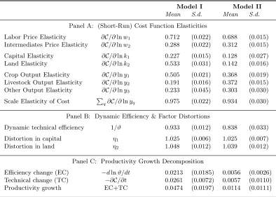
Before proceeding to the discussion of main results concerning dynamic (in)efficiency and factor distortions, we first examine the scale elasticity estimates P_q∂C/∂lnyq. These estimates are of

scale economies

0.8 0.85 0.9 0.95 1 1.05 1.1

density

0 5 10 15

Model I Model II

Figure 1. Distributions of posterior estimates of the scale elasticity of cost

corresponding 95% posterior coverage regions includes unity suggesting that, on average, the agri-cultural farm production sector in the U.S. exhibits constant returns to scale during our sample period, which is consistent with the findings by O’Donnell (2016) who uses similar data for the Northeast in the 1960–1989 period. The alternative Model II however produces qualitatively dif-ferent evidence in favor of significant economies of scale at the aggregate level. This tendency of the second model to under-estimate scale elasticity and thus to over-estimate returns to scale in the sector is distribution-wise as can vividly be seen in Figure 1, which plots sampling distributions of posterior estimates of the scale elasticity of cost from the two models. Further, the empirical results from the two models also non-negligibly differ in other aspects of the cost relationship. Contrasting the posterior estimates of individual mean cost elasticities (see Panel A of Table 1), we find that treating dynamic efficiency as exogenous (in Model II) appears to dramatically under-estimate sensitivity of costs to quasi-fixed factors as well as to indicate a higher relative importance of intermediate inputs (over labor) in the cost.

Panel B of Table 1 presents the estimates of primary interest to our paper. First, consider the dynamic variable-input-oriented technical efficiency ϑ−_t1 ∈ (0,1]. We find that the failure to allow for potential endogenous adjustments in efficiency over time (Model II) produces significantly lower estimates of technical efficiency: the pooled mean posterior estimate of 0.84 vs. 0.93 from our endogenous-efficiency Model I. The posterior results from Model II are also significantly more variable, as can be seen from Figure 2, with more than a few point estimates of around 0.8 and lower. Overall, this tendency of Model II to under-estimate efficiency is likely due to its inherent inability to properly credit producing units for incurring efficiency-improvement adjustment costs.6

6

dynamic efficiency, 1/ϑ

0.65 0.7 0.75 0.8 0.85 0.9 0.95 1

density

0 5 10 15 20 25 30 35 40 45

Model I Model II

Figure 2. Distributions of posterior estimates of the dynamic efficiency

(a) Model I

distortions, η_j

0.99 1 1.01 1.02 1.03 1.04 1.05 1.06 1.07 1.08 1.09

density

0 10 20 30 40 50 60

Capital Land

(b) Model II

distortions, ηj

1 1.01 1.02 1.03 1.04 1.05 1.06 1.07 1.08 1.09

density

0 5 10 15 20 25 30 35 40 45

Capital Land

(a) Technical change

technical change

-0.04 -0.03 -0.02 -0.01 0 0.01 0.02 0.03 0.04 0.05 0.06

density

0 10 20 30 40 50 60

Model I Model II

(b) Efficiency change

efficiency change

-0.04 -0.02 0 0.02 0.04 0.06 0.08

density

0 20 40 60 80 100 120 140

Model I Model II

(c) Productivity change

productivity growth

-0.04 -0.02 0 0.02 0.04 0.06 0.08 0.1 0.12

density

0 5 10 15 20 25 30 35

Model I Model II

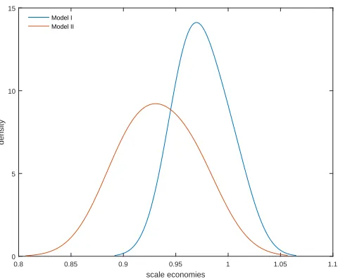
Next, we examine distortions in the use of quasi-fixed inputs. Our empirical results suggest several findings. First, regardless of whether the variable-input efficiency treated as exogenous or endogenous, the data consistently indicate an over-use in both quasi-fixed dynamic inputs as evidenced by universally greater-than-one values of posterior estimates of η1 > 0 for capital and

η2 >0 for land: see Figure 3 that plots their sampling distributions across the two models. Second,

both models indicate a greater degree of over-use in land than physical capital. Third, our preferred Model I produces evidence of somewhat greater distortions in the land use, with the posterior mean estimate of 4.8% compared to that of 3.9% from Model II (see Panel B of Table 1). When it comes to the capital use however, the average distortions are the same across the two models (although the distributions thereof are not).

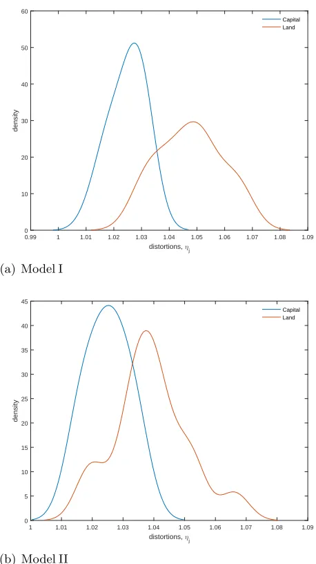
Until now, we have paid little attention to the dynamics in production technology over time. We now specifically focus on temporal changes in agricultural production. The dual cost-function-based productivity growth measure and its decomposition into key components provide a natural avenue for summarizing temporal dynamics in the production. Given our (based on preferred Model I) and the previously reported evidence of unitary returns to scale in the U.S. farm production as well as maintaining our implicit assumption of no allocative inefficiency, the dual multi-output productivity growth index can be easily shown to be a sum of the technical change and efficiency change, with each component respectively defined as−∂lnCt/∂tand−dlnϑt/dt(e.g., see Kumbhakar & Lovell,

2000), which is how we measure it. The posterior mean estimates of productivity growth and its components are reported in Panel C of Table 1; their respective sampling distributions are plotted in Figure 4.

We document stark differences in the productivity growth estimates across the two models. Our preferred endogenous-efficiency Model I estimates the average productivity growth rate in the agricultural farm production at significant 4.7% p.a. whereas the corresponding estimate from the exogenous-efficiency Model II is merely 1.1% and is insignificant. Based on the decomposition results, we find that the latter model produces much smaller close-to-zero estimates of both the mean efficiency and technical change. When endogenizing efficiency however, our results suggest material improvements in dynamic efficiency over time at an about 2.6% average annual rate. Interestingly, our posterior mean estimates of productivity growth in the farm production from Model I are notably greater than those reported earlier by Ball et al. (1997) and more recently by Andersen, Alston, Pardey & Smith (2018) and Plastina & Lence (2018). This may be plausibly attributed to distinct differences in the productivity measurement methodologies. Unlike the cited studies that pursue primal static-production approaches, our methodology is dual and follows a dynamic framework.7

Having contrasted empirical results from the two models, a natural question is which of the two is more favored by the data. The posterior estimate of the efficiency adjustment cost parameter

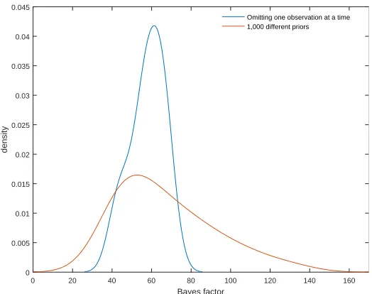
costs.

7

Bayes factor

0 20 40 60 80 100 120 140 160

density

0 0.005 0.01 0.015 0.02 0.025 0.03 0.035 0.04 0.045

Omitting one observation at a time 1,000 different priors

Figure 5. Distributions of the Bayes factor in favor of the endogenous-efficiency model

γo from Model I provides an indirect evidence in favor of the endogenous-efficiency model. We

estimate it to be significantly above zero (see Table A.1 in the Appendix) which lends support to the dynamic endogenization of technical inefficiency ϑt. To select between the two models, we

also employ the Bayes factor constructed using their respective posteriors with that of Model II used in the denominator, implying that the values above one would indicate that Model I is more strongly supported by the data. To ensure robustness of model selection to the choice of priors and the outlier influences in the data, we consider 1,000 alternative prior specifications (via changing hyper-parameters) as well as re-estimate the models using leave-one-out subsamples. Figure 5 plots the corresponding sampling distributions of the Bayes factor, from where it is evident that data overwhelmingly favor our preferred specification that endogenizes dynamic efficiency.

5

Conclusion

procedure that incorporates the variable cost function and both the dynamic and static optimality conditions derived from the firm’s intertemporal expected cost minimization. We operationalize our methodology using a modified version of a nonparametric Bayesian Exponentially Tilted Em-pirical Likelihood adjusted for the presence of dynamic latent variables in the model, which we showcase using the 1960–2004 U.S. agricultural farm production data. Among other things, we find that the failure to allow for potential endogenous adjustments in efficiency over time produces significantly lower estimates of dynamic efficiency, which is likely due to the inherent inability of a more traditional exogenous-efficiency framework to properly credit producing units for incurring efficiency-improvement adjustment costs.

Appendix

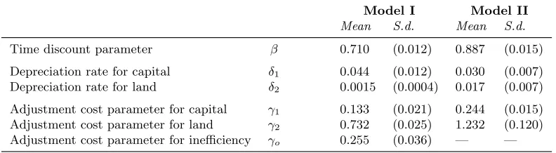
Table A.1. Posterior Estimates of Deep Structural Parameters

Model I Model II

Mean S.d. Mean S.d.

Time discount parameter β 0.710 (0.012) 0.887 (0.015)

Depreciation rate for capital δ1 0.044 (0.012) 0.030 (0.007)

Depreciation rate for land δ2 0.0015 (0.0004) 0.017 (0.007)

Adjustment cost parameter for capital γ1 0.133 (0.021) 0.244 (0.015)

Adjustment cost parameter for land γ2 0.732 (0.025) 1.232 (0.120)

Adjustment cost parameter for inefficiency γo 0.255 (0.036) — —

NOTE: Model I endogenizes dynamic inefficiency, whereas Model II treats it as being exogenous.

References

Ahn, S. C., Good, D. H., & Sickles, R. C. (2000). Estimation of long-run inefficiency levels: A dynamic frontier approach. Econometric Reviews,19, 461–492.

Andersen, M. A., Alston, J. M., Pardey, P. G., & Smith, A. (2018). A century of U.S. farm productivity growth: A surge then a slowdown. American Journal of Agricultural Economics,100, 1072–1090. Andrieu, C. & Roberts, G. O. (2009). The pseudo-marginal approach for efficient Monte Carlo computations.

Annals of Statistics,37, 697–725.

Ball, V. E., Bureau, J., Nehring, R., & Somwaru, A. (1997). Agricultural productivity revisited. American Journal of Agricultural Economics,79, 1045–1063.

Ball, V. E., Gollop, F. M., Kelly-Hawke, A., & Swinand, G. (1999). Patterns of state productivity growth in the U.S. farm sector: Linking state and aggregate models. American Journal of Agricultural Economics,

81, 164–179.

Chen, C.-M. & van Dalen, J. (2010). Measuring dynamic efficiency: Theories and an integrated methodology.

European Journal of Operational Research,203, 749–760.

Doucet, A., Freitas, N., & Gordon, N. (2001). Sequential Monte Carlo Methods in Practice. New York: Springer-Verlag.

Flury, T. & Shephard, N. (2011). Bayesian inference based only on simulated likelihood: Particle filter analysis of dynamic economic models. Econometric Theory, 27, 933–956.

Gallant, A. R., Giocomini, R., & Ragusa, G. (2017). Bayesian estimation of state space models using moment conditions. Journal of Econometrics,201, 198–211.

Gallant, A. R., Hong, H., & Khwaja, A. (2018). A Bayesian approach to estimation of dynamic models with small and large number of heterogeneous players and latent serially correlated states. Journal of Econometrics,203, 19–32.

Girolami, M. & Calderhead, B. (2011). Riemann manifold Langevin and Hamiltonian Monte Carlo methods.

Journal of the Royal Statistical Society B, 73, 123–214.

Gordon, N. J. (1997). A hybrid bootstrap filter for target tracking in clutter.IEEE Transactions on Aerospace and Electronic Systems,33, 353–358.

Gordon, N. J., Salmond, D. J., & Smith, A. F. M. (1993). Novel approach to nonlinear/non-Gaussian Bayesian state estimation. IEEE-Proceedings-F,140, 107–113.

Gould, J. P. (1968). Adjustment costs in the theory of investment of the firm. Review of Economic Studies,

35, 47–55.

Hall, R. E. (2004). Measuring factor adjustment costs. Quarterly Journal of Economics,119, 899–927. Hampf, B. (2017). Rational inefficiency, adjustment costs and sequential technologies. European Journal of

Operational Research,263, 1095–1108.

Kapelko, M. & Oude Lansink, A. (2017). Dynamic multi-directional inefficiency analysis of European diary manufacturing firms. European Journal of Operational Research,257, 338–344.

Kapelko, M., Oude Lansink, A., & Stefanou, S. E. (2014). Assessing dynamic inefficiency of the Spanish construction sector pre- and post-financial crisis.European Journal of Operational Research,237, 349–357. Kapelko, M., Oude Lansink, A., & Stefanou, S. E. (2016). Investment age and dynamic productivity growth

in the Spanish food processing industry. American Journal of Agricultural Economics,98, 946–961. Kapelko, M., Oude Lansink, A., & Stefanou, S. E. (2017). The impact of the 2008 financial crisis on

dynamic productivity growth of the Spanish food manufacturing industry. An impulse response analysis.

Agricultural Economics,48, 561–571.

Kumbhakar, S. C. (1997). Modeling allocative inefficiency in a translog cost function and cost share equations: An exact relationship. Journal of Econometrics,76, 351–356.

Kumbhakar, S. C. & Lovell, C. A. K. (2000).Stochastic Frontier Analysis. Cambridge: Cambridge University Press.

Kumbhakar, S. C., Parmeter, C. F., & Zelenyuk, V. (2017). Stochastic frontier analysis: Foundations and advances. In S. C. Ray, R. Chambers, & S. C. Kumbhakar (Eds.), Handbook of Production Economics, volume 1. Singapore: Springer. forthcoming.

Lambarraa, F., Stefanou, S. E., & Gil, J. M. (2016). The analysis of irreversibility, uncertainty and dy-namic technical inefficiency on the investment decision in the Spanish olive sector. European Review of Agricultural Economics,43, 59–77.

Minviel, J. J. & Sipil¨ainen, T. (2018). Dynamic stochastic analysis of the farm subsidy-efficiency link: Evidence from France. Journal of Productivity Analysis,50, 41–54.

Nemoto, J. & Goto, N. (2003). Measurement of dynamic inefficiency in production: An application of data envelopment analysis to Japanese electric utilities. Journal of Productivity Analysis,19, 191–210. O’Donnell, C. J. (2012). Nonparametric estimates of the components of productivity and profitability change

in U.S. agriculture. American Journal of Agricultural Economics,94, 873–890.

O’Donnell, C. J. (2016). Using information about technologies, markets and firm behaviour to decompose a propose productivity index. Journal of Econometrics,190, 328–340.

Oude Lansink, A., Stefanou, S., & Serra, T. (2015). Primal and dual dynamic Luenberger productivity indicators. European Journal of Operational Research,241, 555–563.

Parmeter, C. F. & Kumbhakar, S. C. (2014). Efficiency analysis: A primer on recent advances. Foundations and Trends in Econometrics,7, 191–385.

Pindyck, R. S. & Rotemberg, J. T. (1983). Dynamic factor demands and the effects of energy price shocks.

American Economic Review,73, 1066–1079.

Pitt, M. K., dos Santos Silva, R., Giordani, P., & Kohn, R. (2012). On some properties of Markov Chain Monte Carlo simulation methods based on the particle filter. Journal of Econometrics,171, 134–151. Plastina, A. & Lence, S. H. (2018). A parametric estimation of total factor productivity and its components

in U.S. agriculture. American Journal of Agricultural Economics,100, 1091–1119.

Ristic, B., Gordon, N., & Arulampalam, S. (2004). Beyond the Kalman Filter: Particle Filters for Tracking Applications Partical Filters for Tracking Applications. Norwood, MA: Artech House.

Rungsuriyawiboon, S. & Stefanou, S. (2007). Primal and dual dynamic Luenberger productivity indicators.

Journal of Business and Economic Statistics,25, 226–238.

Schennach, S. M. (2005). Bayesian exponentially tilted empirical likelihood. Biometrika,92, 31–46.

Sengupta, J. K. (1995). Dynamics of Data Envelopment Analysis. Dordrecht: Kluwer Academic Publishers. Serra, T., Oude Lansink, A., & Stefanou, S. E. (2011). Measurement of dynamic efficiency: A directional

distance function parametric approach. American Journal of Agricultural Economics,93, 756–767. Silva, E. & Oude Lansink, A. (2013). Dynamic efficiency measurement: A directional distance function

approach. Centro de Economia e Finan¸cas da UPorto Working Paper 2013–07.

Silva, E. & Stefanou, S. E. (2003). Nonparametric dynamic production analysis and the theory of cost.

Journal of Productivity Analysis,19, 5–32.

Silva, E. & Stefanou, S. E. (2007). Dynamic efficiency measurement: Theory and application. American Journal of Agricultural Economics,89, 398–419.

Skevas, I., Emvalomatis, G., & Br¨ummer, B. (2018). Productivity growth measurement and decomposi-tion under a dynamic inefficiency specificadecomposi-tion: The case of German dairy farms. European Journal of Operational Research,271, 250–261.

Tsionas, E. G. (2006). Inference in dynamic stochastic frontier models. Journal of Applied Econometrics,

21, 669–676.

Tsionas, E. G. & Izzeldin, M. (2018). A novel model of costly technical efficiency. European Journal of Operational Research,268, 653–664.