Munich Personal RePEc Archive
Exogenous uncertainty and the
identification of Structural Vector
Autoregressions with external
instruments
Angelini, Giovanni and Fanelli, Luca
University of Bologna
May 2018
Online at
https://mpra.ub.uni-muenchen.de/93864/
Exogenous uncertainty and the identi…cation of
Structural Vector Autoregressions with external
instruments
Giovanni Angelini
University Ca’ Foscari of Venice
Luca Fanelli University of Bologna
May 2018. First revision: January 2019; Second revision: May 2019
Abstract
We provide necessary and su¢cient conditions for the identi…cation of Structural Vector Autoregressions (SVARs) with external instruments considering the case in which r instru-ments are used to identify g structural shocks of interest, r g 1. Novel frequentist estimation methods are discussed by considering both a ‘partial shocks’ identi…cation strat-egy, where onlygstructural shocks are of interest and are instrumented, and in a ‘full shocks’ identi…cation strategy, where despite g structural shocks are instrumented, all nstructural shocks of the system can be identi…ed under certain conditions. The suggested approach is applied to empirically investigate whether …nancial and macroeconomic uncertainty can be approximated as exogenous drivers of U.S. real economic activity, or rather as endogenous responses to …rst moment shocks, or both. We analyze whether the dynamic causal e¤ects of non-uncertainty shocks on macroeconomic and …nancial uncertainty are signi…cant in the period after the Global Financial Crisis.
Keywords: Exogenous Uncertainty, External Instruments, Identi…cation, proxy-SVAR, SVAR.
J.E.L.: C32, C51, E44, G10.
1
Introduction
Structural Vector Autoregressions (SVARs) provide stylized and parsimonious characterizations
of shock transmission mechanisms and allow to track dynamic causal e¤ects in empirical
1
Introduction
Structural Vector Autoregressions (SVARs) provide stylized and parsimonious characterizations of shock transmission mechanisms and allow to track dynamic causal effects in empirical macroe-conomics. The identification of SVARs requires parameter restrictions on the matrix which maps
the VAR disturbances to structural shocks, henceforth denoted withB, that are often implausi-ble. The parameters in the matrixBcapture the instantaneous impacts of the structural shocks
on the variables and are crucial ingredients of the Impulse Response Functions (IRFs). One of the most interesting approaches developed in the recent literature to identify structural shocks
by possibly avoiding recursive structures, or implausible assumptions on the elements of B is the so-called ‘external instruments’ or ‘proxy-SVAR’ (or ‘SVAR-IV’) approach, see Stock and Watson (2012, 2018) and Mertens and Ravn (2013, 2014). This method takes advantage of
information developed from ‘outside’ the VAR in the form of variables which are correlated with the latent structural shocks of interest (relevance condition) and are uncorrelated with the other
structural shocks of the system (exogeneity, or orthogonality condition).
The emerging literature on proxy-SVARs (throughout the paper we use the terms ‘SVARs with external instruments’ and ‘proxy-SVARs’ interchangeably) is mainly devoted to the use
of one external instrument to identify a single structural shock of interest in isolation from all the other shocks of the system. For example, Stock and Watson (2012) identify six shocks (the
oil shock, the monetary policy shock, the productivity shock, the uncertainty shock, the liquid-ity/financial risk shock and the fiscal policy shock) by exploiting many external instruments,
but use them one at a time; see also Ramey (2016). Remarkable exceptions are Mertens and Ravn (2013) and Mertens and Montiel Olea (2018) who deal with the case of two instruments and two structural shocks (r=g= 2); see also Ariaset al. (2018b).1 Mertens and Ravn (2013)
show that when g > 1, the restrictions provided by the external instruments do not suffice to identify the shocks and must be complemented with additional constraints. They obtain these
constraints from a Choleski decomposition of a covariance matrix.
In general, there exists no result in the literature which provides a guidance for practitioners
to address the following question: given g ≥ 1 structural shocks of interest in a system of n variables and r ≥ g external instruments available for these shocks, how many restrictions do we need for the model to be identified and where do these restrictions need to be placed? One
main contribution of this article is to provide such a general framework, i.e. we extend the identification analysis of proxy-SVARs to the case in which multiple instruments (r) are used to
identify multiple shocks (g≥1). We show that wheng >1,the additional restrictions necessary
1Actually, Caldara and Kamps (2017) consider the caser=g= 3 and an identification strategy which can be
to identify the shocks of interest (up to sign normalization) other the external instruments need not be Choleski-type constraints. We discuss novel frequentist estimation methods alternative
to instrumental variables (IV) techniques: a classical minimum distance (CMD) approach and maximum likelihood (ML) approach, respectively. Further, we argue that one of the advantages
of covering the case r > g (i.e. the proxy-SVAR features more instruments than shocks of interest) is that a practitioner can potentially include up to r −g weakly relevant (or not relevant at all) external instruments in the proxy-SVAR without affecting the inference if at
leastg instruments are strongly correlated with the structural shocks of interest.
Our approach is based on the idea of augmenting the SVAR with an auxiliary model for ther
external instruments. We obtain a ‘larger’m-dimensional SVAR, withm=n+r, which conveys conveniently all the information relevant to identify thegstructural shocks of interest. This large
system is called the SVAR model, where ‘AC’ stands for ‘augmented-constrained’. The AC-SVAR model is ‘augmented’ because it is obtained by appending the external instruments to the original SVAR equations. The AC-SVAR model is ‘constrained’ because it features a triangular
structure in the autoregressive coefficients and a particularly constrained structure in the matrix that contains the structural parameters (the on-impact coefficients). We discuss two types of
identification strategies which can be accommodated within the AC-SVAR framework depending on the information available to the practitioner: a ‘partial shocks’ identification approach, which
is the typical case in the proxy-SVARs literature, and a ‘full shocks’ identification approach which occurs, under certain conditions, when all structural shocks of the system can be identified by ther external instruments.
In the ‘partial shocks’ identification approach, the objective is to identify the dynamic causal effects of g ≥1 structural shocks of interest using r ≥g valid external instruments, regardless
of the other n−g shocks of the system. When r = g = 1, the parameter which captures the correlation between the external instrument and the shock of interest is a scalar, sayφ, and the parameters which are necessary to estimate the IRFs correspond to a column of the matrix B.
Wheng >1 andr≥gexternal instruments are used,φ= Φ becomes a matrix withr rows andg columns and contains therefore more than one ‘relevance’ parameter. We propose a novel CMD
estimation method for proxy-SVARs based on a set of moment conditions implied by the AC-SVAR model. In particular, we minimize the distance between a set of reduced form parameters,
which can be easily and consistently estimated from the AC-SVAR model, and the parameters which capture the instantaneous impact of the instrumented shocks. The identification of the proxy-SVAR (up to sign) depends on a rank condition associated with the Jacobian matrix
In the ‘full shocks’ identification approach, r valid external instruments are still used to identify (up to sign)g≥1 instrumented structural shocks,r≥g, but it is now possible to infer,
under some additional constraints, the dynamic causal effects of all n structural shocks of the system, including those associated with the n−g non-instrumented shocks. The identification
of the AC-SVAR model in the ‘full shocks’ approach amounts to the practice of identifying an enlarged ‘B-model’ using the terminology in L¨utkepohl (2005) (‘C-model’ using the terminology in Amisano and Giannini, 1997). Estimation can be carried out by ML and requires minor
adaptations to the algorithms discussed in e.g. Amisano and Giannini (1997) and L¨utkepohl (2005) implemented in econometric packages.
Since we treat the proxy-SVAR as a ‘large’ SVAR, in our framework the issue of making bootstrap inference on the IRFs, discussed in Jentsch and Lunsford (2016) and Montiel Oleaet
al. (2018) and recently debated in Jentsch and Lunsford (2019) and Mertens and Ravn (2019), boils down to the problem of making bootstrap inference on the IRFs generated by SVARs, see e.g. Kilian and L¨utkepohl (2017) for a review. For instance, in the empirical application
of Section 8 we first check that the disturbances of the estimated AC-SVAR model are not characterized by conditional heteroskedasticity (because of the results in Br¨uggemann et al.
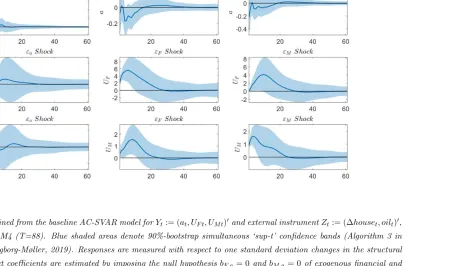
(2016) on inference in SVARs with conditional volatility of unknown form), and then compute simultaneous confidence bands for the IRFs of interest by combining a standard residual-based
recursive-design bootstrap algorithm with the ‘sup-t’ method discussed in Montiel Olea and Plagborg-Møller (2019).
Moreover, when the AC-SVAR system is overidentified, a convenient way to test the
empir-ical validity of the proxy-SVAR model is to compute overidentification restrictions tests. Our analysis shows that these tests tend to reject the proxy-SVAR when the external instruments
are erroneously assumed orthogonal to the non-instrumented shocks. Thus, we have analogs of the ‘Sargan’s specification test’ in the instrumental variables framework, or the ‘Hansen’s J-test’ in the generalized method of moments framework, and this appears a novelty in the literature
on proxy-SVARs. Notably, in the full shocks identification approach, the quality of the identifi-cation can be evaluated not only by checking the relevance condition, but also the orthogonality
between the external instruments and the non-instrumented shocks.
The second contribution of this article is empirical. We apply our methodology to address
a recently debated issue of the uncertainty literature, i.e. whether uncertainty is a driver of the U.S. business cycle or rather a response to first moment shocks, or both. A well recognized fact in the literature is that uncertainty is recessionary in presence of real options effects (e.g.
to first moment shocks, especially during periods of economic and financial turmoil. Indeed, uncertainty appears also to endogenously increase during recessions, as lower economic growth
induces greater dispersion at the micro level and higher aggregate volatility.
Reverse causality between uncertainty and real economic activity using monthly or quarterly
data can not be analyzed by recursive (triangular) SVARs which presume that some variables respond only with a lag to others. This issue has been analyzed in the recent literature by Ludvigson et al. (2018), Carriero et al. (2018) and Angelini et al. (2019). These authors use
non-recursive SVARs and different identification methods and report mixed evidence. We focus on the U.S. economy after the Global Financial Crisis, in particular the ‘Great Recession+Slow
Recovery’ period 2008-2015, and consider a small-scale monthly SVAR which includes measures of macroeconomic and financial uncertainty taken from Jurado et al (2015) and Ludvigson et
al. (2018), respectively, and a measure of real economic activity, say the industrial production growth (n = 3). The scope of our analysis is to investigate whether the selected measures of macroeconomic and financial uncertainty respond on-impact (instantaneously) and/or with lags
to a ‘non-uncertainty’ shock (g= 1). This requires a non-recursive (non-triangular) specification for the matrix B which makes our approach potentially attractive. The direction of causality
we are primarily interested in runs from real economic activity to uncertainty, not the other way around, and this requires the use of valid external instruments for the variable of the
system related to real economic activity. Thus, in our baseline specification we use two external instruments jointly (r = 2) to identify the ‘non-uncertainty’ shock of the system and track its dynamic impact on financial and macroeconomic uncertainty. This strategy differs from e.g.
Stock and Watson (2012) who use valid external instruments (one at a time) to identify the effects of uncertainty shocks on macroeconomic variables. It differs also from Ludvigsonet al. (2018)’s
strategy, where two external instruments for financial and macroeconomic uncertainty shocks are employed to narrow the identification set obtained by directly restricting the structural shocks in correspondence of particular events (event constraints).
The external instruments we employ for the non-uncertainty shock are: (a) the time series innovations obtained from an auxiliary regression models for the changes in the log of new
privately owned housing units started; (b) an oil supply shock identified along the lines of Kilian (2009); (c) the time series innovations obtained from an auxiliary regression model for the
changes in the log of hours worked. The couples of external instruments (a,b) and (a,c) are used to identify the non-uncertainty shock of the system in a partial shocks identification strategy, but also in a full shocks identification strategy under an auxiliary hypothesis on the pass-through
on-impact. Macroeconomic uncertainty does not respond at any lag to the identified real economic activity shocks while financial uncertainty displays a short-lived response after one period, so
that the overall empirical evidence in favor of the hypothesis of ‘endogenous uncertainty’ appears scant. Notably, our analyses provide empirical support to the validity of the selected external
instruments. Admittedly, however, our results can not be considered ‘final’ as they depend on the specific set of external instruments used to identify the non-uncertainty shock.
Our paper is naturally connected with the increasing strand of the macroeconometric
liter-ature which develops and applies estimation and inferential methods for SVARs with external instruments. We compare thoroughly our methodology with other approaches in Sections 7
and our empirical results with other works on exogenous/endogenous uncertainty in Section 8.3. Our approach is based on the maintained assumption that the external instruments are strongly
correlated with the instrumented structural shocks, which might not be the case in applied work. Lunsford (2015) and Montiel Olea et al. (2018) discuss identification-robust inferential methods for weak external instruments. The extension of our approach to proxy-SVARs to weak
instruments is left to future research.
The paper is organized as follows. Section 2 introduces the reference SVAR with external
instruments and presents the main assumptions. Section 3 discusses the AC-SVAR representa-tion of proxy-SVARs and Secrepresenta-tion 4 motivates two identificarepresenta-tion strategies featured by AC-SVAR
models by considering an example centered of the concept of exogenous/endogenous uncertainty in SVAR models. Section 5 deals with the ‘partial shocks’ identification strategy and proposes a CMD estimation approach alternative to IV methods. Section 6 deals with the ‘full shocks’
identification strategy and discusses estimation through ML. Section 7 connects our approach to proxy-SVARs to the literature. Section 8 applies the suggested methodology to investigate the
exogeneity/endogeneity of uncertainty in the U.S. in the period after the Global Financial Crisis. Section 9 contains some concluding remarks. Additional technical details, formal proofs, Monte Carlo experiments and further empirical results are confined in a Supplementary Appendix.
2
SVAR and the auxiliary model for the external instruments
We start from the SVAR system:
Yt= ΠXt+ ΥyDy,t+ut , ut=Bεt , t= 1, ..., T (1)
where Yt is the n×1 vector of endogenous variables, Xt:=(Yt′−1, ..., Y ′ t−k,)
′
with positive definite covariance matrix Σu := E(utu′t). The initial conditions Y0, ..., Y1−k are treated as fixed. The system of equations ut = Bεt in eq. (1) maps the n×1 vector of iid
structural shocks εt, which are assumed to have normalized unit covariance matrix E(εtε′t) := Σε=In, to the reduced form disturbances through the n×n matrixB.2
We call the elements in (Π,Υy,Σu) reduced-form parameters and the elements in B struc-tural parameters or on-impact coefficients. Moreover, we use the terms ‘identification of B’, ‘identification of the SVAR’ and ‘identification of the shocks’ interchangeably. Let
Ay :=
Π1 · · · Πk
In(k−1) 0n(k−1)×n
(2)
be the VAR companion matrix. The responses of the variables inYt+hto one standard deviation structural shock εjt is captured by the IRFs:
IRFj(h):=(Jn(Ay)hJn′)bj , h= 0,1,2, .... (3)
where bj is the j-th column of B, j = 1, ..., n and Jn := (In : 0n×n(k−1)) is a selection matrix such that JnJn′ =In. Standard local and global identification results for the SVAR in eq. (1)
are reviewed in the Supplementary Appendix A.2.
Our first assumption postulates the correct specification of the SVAR and the nonsingularity
of the matrix of structural parametersB, the only formal requirement we place on this matrix, except where indicated.
Assumption 1 (DGP) The data generating process belongs to the class of models in eq. (1)
which satisfy the following conditions:
(i) the companion matrix Ay in eq. (2) is stable, i.e. all of its eigenvalues lie inside the unit
circle;
(ii) the matrix B is nonsingular.
Given Assumption 1 we consider, without loss of generality, the following partition of the
vector of structural shocks:
εt:= ε1,t ε2,t
!
g×1
(n−g)×1 (4)
2The structural shocksεt may also have diagonal covariance matrix Σε :=diag(σ2
1, ..., σn2).In this case, the link between reduced form disturbances and structural shocks can be expressed in the formut=B∗
Σ1ε/2ε∗t, where ε∗
t := Σ −1/2
whereε1,tis theg×1 subvector of structural shocks henceforth denoted ‘instrumented structural shocks’, andε2,tis the (n−g)×1 subvector of other structural shocks, denoted ‘non-instrumented shocks’. The instrumented structural shocks are ordered first for notational convenience only: the ordering of variables is irrelevant in our setup. Given the corresponding partition of reduced
form VAR disturbances, ut := (u′1,t, u ′
2,t), whereu1,t and u2,t have the same dimensions as ε1,t and ε2,t, we partition the matrix of structural parametersB conformably with eq. (4):
B:=
B1
n×g
B2
n×(n−g)
= B11 B12
B21 B22
!
g×g g×(n−g)
(n−g)×g (n−g)×(n−g) . (5)
In eq. (5), the dimensions of submatrices have been reported below and alongside blocks. B1 is
the submatrix containing the on-impact coefficients associated with the instrumented structural
shocks ε1,t, and B2 is the submatrix containing the on-impact coefficients associated with the
non-instrumented shocksε2,t;rank(B1) =gandrank(B2) =n−gbecause of Assumption 1(ii).
The external instruments approach postulates that given the partitions in eq.s (4)-(5), there
are available r ≥ g observable ‘external’ (to the SVAR) variables called instruments, that we collect in the r×1 vector vZ,t, which can be used to identify the dynamic causal effect of ε1,t on Yt+h, h = 0,1, ..., without the need to impose implausible assumptions on the elements of B. Thus, we can consider the instrumented structural shocks in ε1,t as the shocks of primary interest in the analysis and for which r valid external instruments are employed. However, as it will be shown below, there are cases in which despite ε1,t is instrumented, also the ‘other’ structural shocks in ε2,t might be of interest and identified under certain conditions. The key properties of vZ,t are formalized in the next assumption.
Assumption 2 (Relevance and orthogonality) The r×1 vector vZ,t is generated by the
system of equations:
vZ,t=RΦεt+ωt= Φε1,t+ωt (6)
where RΦ := Φ : 0r×(n−g)
,Φis anr×gmatrix of full column rank, and ωt is ar×1
measure-ment error term uncorrelated with εt (E(εtωt′) = 0n×g) with positive definite covariance matrix E(ωtωt′) := Σω <∞.
Assumption 2 ensures that the external instruments invZ,tsatisfy the conditionsE(vZ,tε′1,t) = Φ6= 0r×n(‘relevance’) andE(vZ,tε
′
2,t) = 0r×(n−g) (‘exogeneity’, or ‘orthogonality’).3 These con-ditions are typically presented in the proxy-SVAR literature under the setup r = g, see e.g.
3Assumption 2 is consistent with a scenario in which the external instruments in vZ,t can potentially be
correlated with past structural shocks, i.e. it may hold the condition Cov(vZ,t, εt−i) = E(vZ,tε ′
t−i) 6= 0r×n, i= 1,2, ...which, because of eq. (6), requiresE(ωtε′
Stock and Watson (2012, 2018), Mertens and Ravn (2013, 2014), and require that the elements invZ,tare correlated with the instrumented structural shocksε1,tand are orthogonal to the other shocks in ε2,t.4 The matrix RΦ :=
Φ 0r×(n−g)
in eq. (6) characterizes the instruments validity as it collects the relevance and orthogonality conditions. We call Φ the ‘relevance
ma-trix’ (or ‘matrix of relevance parameters’) thoughout the paper. The condition rank(Φ) =g in Assumption 2 ensures that each column of Φ carries independent - not redundant - information on the instrumented structural shocks. It will be shown in the next sections thatrank(Φ) =gis
a necessary condition for identification which becomes also sufficient when g= 1. The additive measurement errorωtin eq. (6) captures the idea that the external instruments are imperfectly
correlated with the instrumented structural shocks; the covariance matrix Σω can be possibly diagonal.
The ‘one shock-one instrument’ case mainly treated in the proxy-SVAR literature obtains for r=g= 1 and implies thatRΦ:=φ 1 : 01×(n−1)
in eq. (6) is a row and Φ =φis a scalar. In this paper we focus on the general caser ≥g≥1 and explore the consequences of such generalization
on the identification and (frequentist) estimation of proxy-SVARs. By considering the general case r ≥ g ≥ 1, we mimick the situation that occurs in the instrumental variable regressions
when the number of instruments can be larger than the number of estimated parameters. As it will be shown next, whenr > g, (r−g) external instruments might be weakly correlated (or not
correlated at all) with theginstrumented shocks without consequences on asymptotic inference if at leastg external instruments are strongly correlated with the instrumented shocks.
To present our method it is convenient to generalize the auxiliary model for the external
instruments postulated in eq. (6). Indeed, the data generating process specified for vZ,t in Assumption 2 maintains that the dynamics of the external instruments is expressed in ‘innovation
form, asvZ,tdepends on the instrumented structural shocksε1,tand the measurement errorωt. In some situations, however, the practitioner might observe anr×1 vector of ‘raw’ (stationary) time dependent time series whose innovation part might potentially serve as external instruments.
To account for these situations, we interpretvZ,t as the innovation part of Zt, i.e. the quantity vZ,t :=Zt−E(Zt | Ft−1), where Ft−1 is the econometrician’s information set available at time t−1. A specification consistent with the decompositionZt=E(Zt| Ft−1) +vZ,tis given by the dynamic system:
Zt= Θ(L)Zt−1+ Γ(L)Yt−1+ ΥzDz,t+ Υz,yDy,t+vZ,t (7)
where Θ(L) := Θ1+...+ ΘpLp−1 is a matrix polynomial in the lag operatorL, whose coefficients 4Henceforth, the exogeneity of the external instruments with respect to the non-instrumented shocks will
are in ther×rmatrices Θi,i= 1, ..., p(and can be possibly zero); Γ(L) := Γ1+Γ2L+...+ΓqLq−1 is a matrix polynomial in the lag operator L whose coefficients are in the r ×n matrices Γj,
j= 1, ..., q (and can be possibly zero);Dz,tis an dz-dimensional vector containing deterministic components (constant, dummies, etc.) specific to Ztand not included in Dy,t; Υz and Υz,y are
ther×dz andr×dy matrices of coefficients associated withDz,tandDy,t,respectively (an can be possibly zero).
Equation (7) defines our auxiliary statistical model for the external instruments. It reads as
a reduced form system whereZt may depend on its own lags Zt−1, ...,Zt−p, the predetermined ‘control’ variables Yt−1, ..., Yt−k, and a set of deterministic terms. Obviously, Zt ≡ vZ,t when all coefficient of the system in eq. (7) are zero, meaning that the elements in Zt are already in innovations or iid shocks taken from other studies (see Section 8). When the Θi are non-zero,
the stability requirement assumed for the SVAR (Assumption 1) is extended toZt and requires that the roots of det(Ir−Θ1s−...−Θpsp) = 0 satisfy the condition|s|>1.With this in mind, in the following we call ‘external instruments’ Ztand vZ,t interchangeably.5
In the next section, the SVAR in eq. (1) will be combined with the auxiliary model in eq. (7) to form a ‘larger’ system which incorporates the dynamics of the external instruments in a
coherent and efficient way.
3
The AC-SVAR representation
By coupling the SVAR in eq. (1) with the auxiliary model for the external instruments in eq. (7) we obtain the system:
Yt Zt
!
= ℓ
X
j=1
Πj 0n×r Γj Θj
!
Yt−j Zt−j
!
+ Υy 0n×dz
Υz,y Υz
!
Dy,t Dz,t
!
+ ut
vZ,t
!
(8)
ut
vZ,t
!
= B 0n×r
RΦ Σ1ω/2
!
εt
ω◦ t
!
(9)
5Some of the external instruments inZt (vZ,t) might be censored as in the case of narrative time series, see
e.g. Mertens and Ravn (2013). The Supplementary Appendix A.11 summarizes how the approach presented in this paper can be amended to account for external instruments which are generated by censored autoregressive
processes. A full treatment of this issue deserves a detailed analysis which goes beyond the scopes of the present article and is therefore postponed to future research. To our knowledge, Mertens and Raven (2013) and Jentsch and Lunsford (2019) are examples in which censoring is excplicitly accounted for in the current proxy-SVARs
where ℓ := max{k, p, q} , Σ1ω/2 denotes the symmetric square root of the matrix Σω and the term ω◦
t := Σ −1/2
ω ωt can be here interpreted as a normalized measurement error.6 System (8) reads an m-dimensional VAR, m := n+r, of lag order ℓ which incorporates a constrained (triangular) autoregressive structure: the lags of Zt and the deterministic variables in Dz,t are
not allowed to enter theYt-equations of the original SVAR. The matrices Γj and Θj,j= 1, ..., ℓ and Υz,y and Υz are restricted to zero in eq. (8) when Zt ≡ vZ,t. System (9) maps the term
ξt:= (ε′t, ω ◦′ t )
′
(which includes the structural shocks) ontoηt:= (u′t, v ′ Z,t)
′ .
It is seen that the joint system (8)-(9) forms a large ‘B-model’ (L¨utkepohl, 2005) which we call the ‘augmented-constrained’ SVAR (AC-SVAR) model. For future reference, we compact
the AC-SVAR model in the expression:
Wt=ΨFe t+ΥDe t+ηt , ηt=Gξe t (10)
where Wt := (Yt′, Z ′ t)
′
and ηt := (u′t, v ′ Z,t)
′
are m ×1, the reduced form disturbance ηt has covariance matrix Ση :=E(ηtη′t), Ft:= (Wt′−1, ..., W
′ t−ℓ)
′
is f×1 (f =mℓ), Ψ := (e Ψe1, ...,Ψeℓ) is m×f,Dt:= (Dy,t′ , D
′ z,t)
′
isd×1 (d:=dy+dz),Υ ise m×dand, finally,ξt:= (ε′t, ω ◦′ t )
′
ism×1.
We use the symbol ‘∼’ over the matrices Ψ and Υ and G to remark that these are restricted. The structure of the matrix Ge deserves special attention:
e
G:= B 0n×r RΦ Σ1ω/2
!
= B1 B2
Φ 0r×(n−g) 0n×r
Σ1ω/2
!
. (11)
It is seen that Ge contains the structural parameters in B, the relevance and (the zero) orthog-onality conditions embedded in RΦ and the parameters of the matrix Σ1ω/2. The covariance restrictions implied by the AC-SVAR model (the ones stemming from Ση =GeGe′) boild down to
Σu =BB′ SVAR symmetry (12)
ΣvZ,u= ΦB
′
1 External instruments (13)
ΣvZ = ΦΦ
′
+ Σω External instruments. (14)
In the next sections we use the AC-SVAR model and the mapping in eq.s (12)-(14) to derive
general necessary and sufficient conditions for identification and to put forth a novel estimation approach for proxy-SVARs.
6Alternatively we might replace the square root matrix Σ1/2
ω with e.g. the Choleski factor of Σω, Pω, and normalize the measurement errorωtasω◦
t :=P −1
4
Motivating example: exogenous/endogenous uncertainty in a
small-scale SVAR
In this section we motivate empirically two types of identification strategies that the AC-SVAR model may feature. We discuss the exogeneity/endogeneity of measures of uncertainty with respect to the business cycle in a small-scale SVAR model, a topic which will be addressed
empirically in Section 8 on U.S. monthly data.7
Consider a SVAR model for Yt:=(at, UF,t, UM,t)′ (n = 3), where at is a measure of real
economic activity,UF,ta measure of financial uncertainty andUM,ta measure of macroeconomic uncertainty. The relationship between the reduced form disturbances and the structural shocks
is given by:
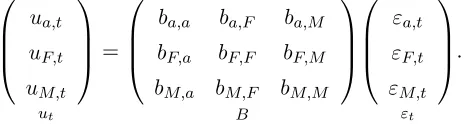
ua,t uF,t uM,t
ut
=
ba,a ba,F ba,M bF,a bF,F bF,M bM,a bM,F bM,M
B
εa,t εF,t εM,t
εt
(15)
whereut:=(ua,t, uF,t, uM,t)′is the vector of VAR reduced form disturbances andεt:= (εa,t, εF,t, εM,t)′
is the vector of structural shocks. As is know, this SVAR is not identified in the absence of (at least three) restrictions on the matrix B. To inform the discussion, we temporarily labelεa,t as the ‘non-uncertainty shock’, εF,tas the ‘financial uncertainty shock’ and εM,t as the
‘macroeco-nomic uncertainty shock’.
Since the seminal paper of Bloom (2009), attention in the empirical literature on uncertainty
has been focused on measuring the impact of uncertainty shocks on real economic activity, which requires the identification of the parameters ba,F and ba,M in eq. (15). For instance, Stock
and Watson (2012) use either stock market volatility or the economic policy uncertainty index of Baker et al. (2016) as external instruments to identify the effects of uncertainty shocks. In their framework, the parameters of interest are in the column bM:=(ba,M, bF,M, bM,M)′ (or
bF:=(ba,F, bF,F, bM,F)′) of the matrixB. In this paper, we are interested in the other direction of causality, namely the impact of εa,t on the variablesUF,t+h and UM,t+h forh= 0,1, .... The on-impact responses (h = 0) are captured by the parameters bF,a and bM,a contained in the first column ba:=(ba,a, bF,a, bM,a)′ of B; the lagged responses (h = 1,2, ...) can be inferred from the IRFs in eq. (3) by setting bj = ba. As in Angelini et al. (2019), we consider financial
and macroeconomic uncertainty ‘exogenous’ if UF,t and UM,t do not respond to εa,t on-impact, which corresponds to the hypothesisbF,a= 0 andbM,a = 0 in eq. (15). Conversely, we consider
financial and macroeconomic uncertainty ‘endogenous’ if UF,t and UM,t respond significantly
7As an exercise, the Supplementary Appendix A.4 applies the two identification strategies to a monetary SVAR
on-impact to the non-uncertainty shock; see Carrieroet al. (2018) for a similar characterization. Obviously, it may happen that UF,t+h and UM,t+h respond to εa,t only after some periods the shock occurs, hence we distinguish between ‘contemporaneous exogeneity’ and lagged effects throughout the paper.
The reverse causality problem can not be addressed by placing ‘conventional’ restrictions on the matrix B in eq. (15). Ludvigson et al. (2018), Angelini et al. (2018) and Carriero et al. (2018) face this issue by estimating non-recursive SVARs identified by different methods
briefly reviewed in Section 8.3. In this paper, we argue that our proxy-SVAR approach can be a valuable alternative to the existing methods.
Partition the structural relationships in eq. (15) as follows:
ua,t uF,t uM,t ut = ba,a bF,a bM,a
B1≡ba
(εa,t) ε1,t
+
ba,F ba,M
bF,F bF,M bM,F bM,M
B2 εF,t εM,t !
ε2,t
(16)
which means that the structural shock of interest, and for which valid external instruments must
be found is the non-uncertainty shock, i.e. ε1,t := (εa,t) (g = 1). Here B1 ≡ba coincides with the first column ofB and contains the parameters of primary interest. Consider, as an example,
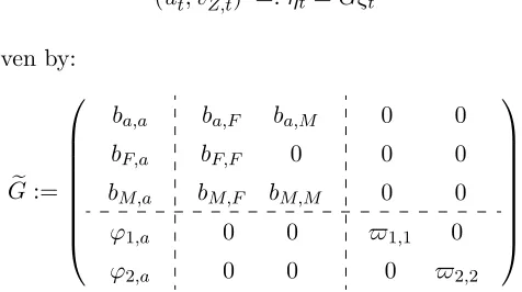
the case in whichr = 2 valid external instruments, collected in the vector Zt(vZ,t), are used for εa,t. The matrix Ge of the AC-SVAR model in eq. (11) reads:
e
G:= Ge1 Ge2
= B1 B2
Φ 02×2 03×2 Σ1̟/2
! = ba,a bF,a bM,a
ba,F ba,M
bF,F bF,M bM,F bM,M
ϕ1,a ϕ2,a
0 0 0 0 0 0 0 0 0 0
̟1,1 ̟2,1
̟2,1 ̟2,2
(17)
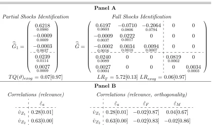
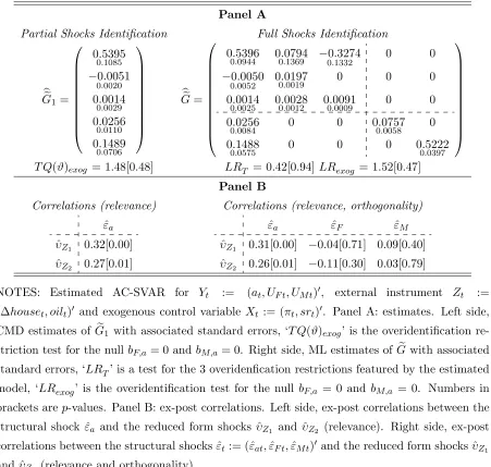
whereϕ1,a:=E(vZ1,tεa,t) andϕ2,a:=E(vZ2,tεa,t) are the relevance parameters contained in the 2×1 matrix Φ, and̟1,1,̟2,1,̟2,2 are the 3 free elements of Σ1̟/2 (assumed here non-diagonal); recall from the previous section that Σ̟ is the covariance matrix of the measurement errorsωt
in eq. (6) and that with Σ1̟/2 we denote the ‘square root’ of Σ̟. Observe that in eq. (17),
e
G1:=(b′a, ϕ ′
)′
, whereba:=(ba,a, bF,a, bM,a)′ and ϕ:= (ϕ1,a, ϕ2,a)′.
The ‘partial shocks’ identification strategy identifies the parameters in the columnGe1:=(b′a, ϕ ′
)′ , hence the shock εa,t, regardless of the other shocks of the system. The idea is that Ge1 is the
only ingredient (other than the reduced form parameters) necessary to track the dynamic causal effect ofεa,tonUF,t+handUM,t+h,h= 0,1, .... The other columns ofG, collected ine Ge2, are not
σv2Z
2 are the main diagonal elements of ΣvZ, the quality of the identification can be evaluated in this case by computing the measures ˆϕ1,a/ˆσvZ1 and ˆϕ2,a/ˆσvZ2, where ˆϕ1,a, ϕˆ2,a, ˆσvZ1 and ˆσvZ2
are consistent estimates of the parameters ϕ1,a, ϕ2,a,σvZ1 and σvZ2, respectively. In Section 5 we study the identification and estimation of the proxy-SVAR considering the caser ≥g≥1.
Suppose now that we have a some (limited) information on the non-instrumented structural shocks whose instantaneous effects are captured by the columns of the matrixB2 in eq. (17). In
particular, based on the results in Angelini et al. (2019), we claim that in the period after the
Global Financial Crisis, the contemporaneous pass-trough between financial and macroeconomic uncertainty is one-way and runs from financial uncertainty to macroeconomic uncertainty, which
implies bF,M = 0 in eq. (17). While the original SVAR forYt:=(at, UF,t, UM,t)′ is not identified with bF,M = 0 in eq. (15), the AC-SVAR model based on Ge in eq. (17) and the additional restriction bF,M = 0 is identified (see Section 8.2). The consequence of this result is that although the structural shock of primary interest is the non-uncertainty shockε1,t := (εa,t), we can also identify the financial and macroeconomic uncertainty shocks inε2,t := (εF,t, εM,t)′. We call this scenario the ‘full shocks’ identification strategy, which is studies in Section 6. Since both ε1,t := (εa,t) and ε2,t := (εF,t, εM,t)′ can be identified, one can obtain ˆεt:= Bb−1uˆt,t = 1, ..., T, where ˆut are the reduced form VAR residuals and Bb is a consistent estimate of B recovered from G. Accordingly, one way to evaluate the quality of the identification is computing thebe measures of strengthCorr(ˆvZ1,t,εˆa,t) andCorr(ˆvZ2,t,εˆa,t) which should be significant with valid instruments, but also the correlations Corr(ˆvZ1,t,εˆF,t), Corr(ˆvZ1,t,εˆM,t), Corr(ˆvZ2,t,εˆF,t) and Corr(ˆvZ2,t,εˆM,t) which should not be statistically significant.8 In this example, the ‘price to pay’ to move from a partial to a full shocks identification approach is given by the auxiliary restriction bF,M = 0, which appears a modest cost relative to the benefits. In general, the investigator is
required to take a (minimal) stand also on the structure of B2 to identify all shocks.
5
Partial shocks identification and estimation strategy
In the partial shocks identification strategy, the objective of the analysis is to exploit the instru-ments inZt (vZ,t) to solely identify the dynamic causal effects of the g instrumented shocks in
ε1,t, ignoring the other shocks collected in ε2,t. This amounts to identify the submatrix B1 in
eq. (5), which in turn provides the IRFs in eq. (3) for j= 1, ..., g,g < n.
Our analysis starts from the AC-SVAR representation of the proxy-SVAR summarized in
8Alternatively, one can compute F-type tests from regressions of the form ˆvZ,t=C
1ˆε1,t+C2εˆ2,t+ǫt,t= 1, ..., T,
where the rejection ofH0R :C1 = 0r×g indicates that the relevance condition is supported by the data, and the non-rejection ofHO
eq.s (10)-(11). We are interested in the firstg columns of the matrix G:e
e
G1 :=
B1
Φ
!
, (18)
while the remainingm−gcolumns inGe2are not of interest. The identification of thegcolumns
of Ge1 in eq. (18) reads as a partial identification exercise which requires imposing at least
1/2g(g−1) restrictions onGe1 (i.e. onB1 and Φ); obviously, no restriction is needed wheng= 1.
This necessary order condition for identification clearly shows that when g > 1, the r external instruments alone do not suffice to identify the shocks of interest, see e.g. Mertens and Ravn (2013), Mertens and Montiel Olea (2018) and Ariaset al. (2018b). In principle, conditional on
the validity of a rank condition we discuss below, the additional restrictions can be placed on the columns of B1 leaving Φ free, or can be imposed on the columns of Φ (preserving the full
column rank condition) leaving B1 free, or possibly can be distributed on bothB1 and Φ.
It turns out that when the restrictions onGe1 are homogenous (i.e. there are zero restrictions
only) and separable across columns, one can check the identification of the proxy-SVAR by referring to the sufficient conditions for global identification established by Theorem 2 in Rubio-Ramirez et al. (2010). However, Theorem 2 in Rubio-Ramirez et al. (2010) provides only
sufficient conditions for identification which are valid when the restrictions are homogeneous and separable across columns. To derive necessary and sufficient conditions for identification
which are valid in more general situations, including the case of non-homogeneus, cross-columns restrictions, we find it convenient to exploit a set of moment conditions implied by the AC-SVAR model which pave the way for a CMD estimation approach.
The Supplementary Appendix A.5 shows that by using simple algebra the moment conditions in eq.s (12)-(13) can be transformed into:
Ξ = ΦΦ′
, ΣvZ,u = ΦB
′
1 (19)
where Ξ := ΣvZ,uΣ
−1
u Σu,vZis anr×rsymmetric matrix (of rankg) which is positive definite when
r=g and is positive semidefinite whenr > g. The advantage of the representation in eq. (19),
relative to that in eq.s (12)-(13) is that the nuisance parameters inB2 have been marginalized
out. The moment conditions in eq. (19) can be formally compacted in the expression:
ζ =f(ϑ) (20)
where ζ := (vech(Ξ)′
, vec(ΣvZ,u)
′ )′
is a vector whose elements depend on the reduced form parameters σ+
η := vech(Ση) of the AC-SVAR model, f(ϑ) := (vech(ΦΦ′)′, vec(ΦB1′)
′ )′
is a
elements in the matrixGe1in eq. (18). The restrictions necessary to identifyGe1are parameterized
in explicit form by:
β1 :=vec(B1) =SB1α1+sB1 , φ:=vec(Φ) =SΦϕ (21)
where α1 is the e1×1 vector which collects the unrestricted (free) elements of β1, e1 ≤ ng,
SB1is anng×e1 full column rank selection matrix and and sB1 is an ng×1 vector containing zeros or known non-zero elements; ϕ is the c×1 vector which collects the unrestricted (free) elements of Φ, c≤rg, and SΦ is an rg×cfull column-rank selection matrix. Obviously, when
β1 is unrestricted, β1 ≡α1,e1≡ng,SB1 ≡Ing andsB1 ≡0ng×1; whenφis unrestricted,φ≡ϕ, c = rg and SΦ ≡ Irg. Because of the presence of the possibly non-zero term sB1, eq. (21) accommodates also non-homogeneous restrictions, which means that some elements of B1 can
be e.g. fixed to known non-zero constants. It is seen that ϑ:= (α′
1, ϕ
′ )′
is (e1+c)×1.
Equation (20) defines a ‘distance’ between thea×1 (a:= 1/2r(r+ 1) +nr) vector of reduced
form parameters ζ and the (e1 +c)×1 vector of parameters ϑ. From Rothenberg (1971) it
follows that necessary and sufficient condition forϑbeing uniquely recovered from ζ is that the
a×(e1+c) Jacobian matrix ∂ϑ∂f′ :=̥ϑ is regular and of full column rank in a neighborhood of
the true value of ϑ.9 We derive the Jacobian matrix̥ϑ below.
Under Assumption 1, the estimator of the reduced form parameter σ+
η of the AC-SVAR model is consistent and asymptotically Gaussian, hence we have the result:
T1/2(ˆζT −ζ0)→dN(0a×1, Ωζ) (22)
where ζ0 denotes the true value of ζ, Ωζ is an a×acovariance matrix which can be estimated consistently (see Supplementary Appendix A.5 for details) and ‘→d’ denotes convergence in distribution. The convergence in eq. (22) involves the estimator of the reduced form parameters
of the AC-SVAR model and is valid also if the matrix of relevance parameters Φ is zero, i.e. irrespective of whether the external instruments are strongly, weakly or not correlated at all
with the structural shocks of interest. This result motivates a robust indirect test for the null hypothesis of ‘no relevance’ based on the idea that if in eq. (19) it is assumed that B1 6= 0n×g, the null hypothesisH0 :vec(Φ) = 0rg×1 (no relevance) is equivalent toH
′
0 :vec(ΣvZ,u) = 0rn×1 (no correlation between the external instruments and the VAR disturbances). We discuss a simple Wald-type test forH′
0 in the Supplementary Appendix A.9.
Given eq.s (20) and the consistency of ˆζT,ϑcan be estimated by solving the CMD problem:
min
ϑ (ˆζT −f(ϑ)) ′b
Ω−1
ζ (ˆζT −f(ϑ)) (23)
9LetM =M(θ) be a matrix of rankm, whose elements depend onθ. M is ‘regular’ ifrank(M(θ)) =min a
where Ωbζ is a consistent estimate of Ωζ. The properties of the estimator ˆϑT obtained from eq. (23) depend on the identification of the proxy-SVAR. The next proposition formalizes the
necessary and sufficient rank conditions and the necessary order condition for the identification of the proxy-SVAR.
Proposition 1 [Partial shocks identification] Given the SVAR in eq. (1), a vector of r external instrumentsvZ,t for the 1≤g < nstrucutral shocks in ε1,t and Assumptions 1-2, consider the identification of theg columns of Ge1 in eq. (18). Letϑ0 := (α′1,0, ϕ
′
0)
′
be the
true value ofϑ:= (α′
1, ϕ
′ )′
. Then:
(a) necessary and sufficient rank condition for identification is
rank{̥ϑ
0}=e1+c where̥ϑ
0 is the Jacobian matrix:
̥ϑ:= 01/2r(r+1)×ng 2D
+
r(Φ⊗Ir) (In⊗Φ)Kng (B1⊗Ir)
!
SB1 0ng×c
0rg×e1 SΦ
!
(24)
evaluated in a neighborhood ofϑ0 and is ‘regular’;10
(b) necessary order condition is that at least 1/2g(g−1) restrictions are placed on the g columns ofGe1, which is equivalent to the conditione1+c≤g(n+r)−1/2g(g−1).
Proof: Supplementary Appendix A.3.
Some remarks are in order.
First, Proposition 1 provides an alternative to Mertens and Ravn’s (2013) identification
approach for proxy-SVARs with g > 1 multiple shocks. Mertens and Ravn (2013) show that wheng >1, the restrictions implied by the external instruments do not suffice alone to identify theg shocks of interest and must be complemented with additional constraints. In their setup,
the 1/2g(g−1) additional constraints necessary to identify the proxy-SVAR stem from the mechanics of the IV approach and are obtained from a Choleski decomposition of a symmetric
matrix. In our framework, the fact that it is necessary to impose at least 1/2g(g−1) restrictions to identify thegshocks of interest is a necessary order condition, but these restrictions need not
be Choleski-type constraints (the Supplementary Appendix A.7 compares in detailed Mertens
10Given the n×g matrix M, Kng denotes the ng×ng commutation matrix which satisfies Kngvec(M) =
vec(M′
). Dn+:=(D ′
nDn)−1D′
ndenotes the Moore-Penrose inverse ofDn, whereDnis then2×12n(n+1)duplication
and Ravn’s (2013) identification approach with ours). Proposition 1 establishes necessary and sufficient conditions for the identification of the parameters in Φ andB1 (i.e. ofGe1) which hold
up to sign normalization, which means that if e.g. a given ˜Φ satisfies the restriction Ξ = ˜Φ ˜Φ′ in eq. (19), also the matrix ˜Φ∗
6
= ˜Φ, obtained from ˜Φ by changing the sign of one or more than
one of its columns, will satisfy eq. (19).
Second, according to Proposition 1(b), the proxy-SVAR is exactly identified whene1+c =
g(n+r)−1/2g(g−1) , i.e. when there are exactly 1/2g(g−1) restrictions on the elements ofGe1
in eq. (18), and is overidentified (and therefore testable) whene1+c < g(n+r)−1/2g(g−1).11
Third, Proposition 1 clarifies that in general, the full column rank condition of the matrix Φ
(Assumption 2) is only necessary for identification. Indeed, the (2,1) block (In⊗Φ)Kng of the Jacobian matrix in eq. (24) suggests that rank{Φ}=g is necessary forrank{(In⊗Φ)Kng}=
ng, which in turn is a necessary condition forrank{̥ϑ0}=e1+c. The structure of̥ϑalso shows
that wheng= 1, the full column rank condition of Φ is also sufficient for the identification of the proxy-SVAR (whateverr). This is easily seen in the ‘one shock-one instrument’ caser=g= 1,
where Φ =φ=ϕis a scalar (c= 1) and ifβ1 is unrestricted (β1 ≡α1) the Jacobian̥ϑcollapses to the (n+ 1)×(n+ 1) matrix:
̥ϑ:=
0 0 · · · 0 2ϕ
ϕIn α1
;
it is seen that ϕ = φ 6= 0 is necessary and sufficient for identification.12 The form of the
Jacobian in eq. (24) also shows that one of the advantages of using more than one instrument to identify a single shock of interest, r > g = 1, is that rank(Φ) = 1 if at least one component in Φ := (ϕ1, ..., ϕr) is different from zero, which means that provided at least one external instrument is strongly correlated with the shock of interest, r−1 external instruments might potentially violate the relevance condition. This argument can be easily generalized to the case
r > g >1.
Coming back to the estimation problem (23), under Assumptions 1-2 and the conditions of
Proposition 1 we have (Newey and McFadden, 1991):
T1/2( ˆϑT −ϑ0)→dN(0(e1+c)×1, Ωϑ) , Ωϑ:=
̥′ϑ Ω−1
ζ ̥ϑ
−1
(25)
11Whenr=gone has a= 1/2g(g+ 1) +ng and e
1+c=g(n+g)−1/2g(g−1) = 1/2g(g+ 1) +gn under
exact identification, hence the Jacobian matrix in eq. (24) is square. Instead, whenr > g, the Jacobian matrix in eq. (24) is ‘tall’ (meaning that it has more rows than columns) even in the case of exact identification, i.e. a= 1/2r(r+ 1) +nr=r2−1/2r(r−1) +nr > g(n+r)−1/2g(g−1) =e
1+c.
12The structure of this Jacobian matrix shows that if the true value ofϕsatisfies the local-to-zero embedding:
ϕ0 :=T1/2̺,̺6= 0, the proxy-SVAR is not identified asymptotically. We refer to Lunsford (2015) and Montiel
where the asymptotic covariance matrix Ωϑcan be estimated consistently byΩbϑ,T :=
ˆ
̥′
ϑ Ωb −1 ζ ̥ˆϑ
−1
and ˆ̥ϑ is taken from eq. (24) by replacing the unconstrained (free) elements inB1 and Φ with
the corresponding elements in ˆϑT := (ˆα′1,T,ϕˆ ′ T)
′ .
When according to Proposition 1 the proxy-SVAR model is overidentified, the CMD problem delivers a test of overidentifying restrictions because, under the null hypothesis ζ0 =f(ϑ0) and
Assumptions 1-2 the quantity T Q( ˆϑT) converges asymptotically to a χ2(l) random variable with l :=g(n+r)−1/2g(g−1)−(e1+c) degree of freedoms. In the IV (GMM) framework,
when the number of instruments (moment conditions) is larger than the number of estimated
parameters, it is possible to compute Sargan’s specification test (Hansen’s J-test), which is typically interpreted as a specification test for the estimated model. The T Q( ˆϑT) test can be
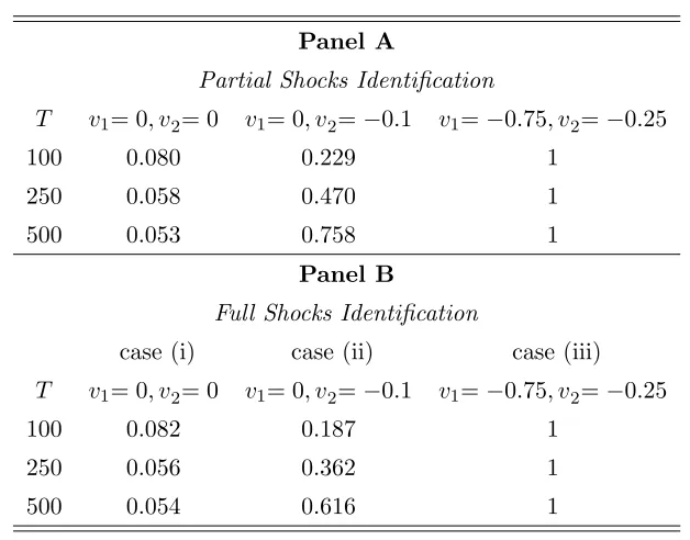
used similarly. Our Monte Carlo experiments (summarized in the Supplementary Appendix A.8 to save space) show that the test T Q( ˆϑT) rejects the overidentification restrictions when the external instruments are incorrectly assumed orthogonal to the non-instrumented structural
shocks.
In case of exact identification, or when the overidentification restrictions are not rejected by
the T Q( ˆϑT) test, the IRFs of interest in eq. (3) can be estimated by replacing the compan-ion matrix Ay with its consistent estimate Aby derived from the AC-SVAR model and bj with the j-th column of Bb1, for j = 1, .., g, where Bb1 is reconstructed from ˆβ1,T:=SB1αˆ1,T +sB1. We refer to Jentsch and Lunsford (2019) and Mertens and Ravn (2019) for a recent debate on bootstrap inference for IRFs in proxy-SVARs; see also Montiel Olea et al. (2018). Since in
our framework the proxy-SVAR is specified as a large (constrained) SVAR ‘B-model’, bootstrap confidence bands for the IRFs can be obtained by applying the methods currently available for
SVARs reviewed e.g. in Kilian and L¨utkepohl (2017, Ch. 12). In particular, when the distur-bances ηt := (u′t, vZ,t′ )
′
in eq. (10) are conditionally homoskedastic, it is possible to combine residual-based bootstrap methods with the CMD approach by the algorithm summarized in the
Supplementary Appendix A.10. Accordingly, the (innovations associated with the) external in-struments are resampled jointly with the VAR residuals regardless of the number of inin-struments
r and instrumented structural shocks g. For instance, in Section 8 we compute 90%-bootstrap simultaneous confidence bands for the IRFs by using the ‘sup-t’ bands discussed in Montiel
Olea and Plagborg-Møller (2019). If instead the disturbances ηt in eq. (10) display conditional heteroskedasticity of unknown form, the results in Bruggemann et al. (2016) and Jentsch and Lunsford (2016, 2019) suggest that reliable inference must be based on the residual-based moving
6
Full shocks identification and estimation strategy
In this case we investigate the conditions under which the instrumentsZt (vZ,t) used to identify the structural shocks of interestε1,tpermit to identify the dynamic causal effects of all structural shocks inεt, including the non-instrumented ones inε2,t.13 We formalize the identification anal-ysis and estimation of proxy-SVARs in these situations and show that (frequentist) estimation of these models can be conveniently carried out by ML.
As in the partial shocks approach, our starting point is the AC-SVAR representation of the proxy-SVAR summarized in eq.s (10)-(11). This is a large ‘B-model’ whose identification depends
on the (number and structure of) restrictions which characterize the matrix G. Equation (11)e shows that Ge incorporates by construnction r(n−g) +nr zero restrictions plus the symmetry constraints stemming from the matrix Σ1ω/2; however, these restrictions do not generally suffice to achieve the at least 1/2m(m−1) restrictions necessary to identify the m columns of G. Ite turns out that aside from special cases discussed below we also need a few restrictions on B2,
other than on B1 and Φ. In the uncertainty example discussed in Section 4, if one adds the
constraint bF,M = 0 in the sub-matrixB2 ofGe in eq. (17), and if e.g. the covariance matrix of
measurement errors Σω is diagonal (which implies ω12 = ω21 = 0), there are 13 homogeneous
restrictions in Ge which are separable across columns (there are therefore 3 overidentification restrictions); it is possible to prove that in this case the model is identified (globally) according
to Theorem 1 in Rubio-Ramirezet al. (2010).
In general, when the restrictions on Ge are homogeneous and separable across columns, it is convenient to study the identification of the AC-SVAR model by checking whether the sufficient conditions for (global) identification in Theorem 1 of Rubio-Ramirez et al. (2010) are satisfied. We derive necessary and sufficient conditions for (local) identification which are valid in more
general situations, including the case of non-homogeneus, cross-columns linear restrictions. To do so, we formalize the restrictions onB1 and Φ as in eq. (21) but, in addition, we include also
restrictions on B2 and Σ1ω/2 as follows:
β2 :=vec(B2) =SB2α2 +sB2, ω:=vech(Σ
1/2
ω ) =SΣω̟. (26)
In eq. (26), α2 is the vector collecting the e2 unrestricted (free) elements ofB2 (if any),SB2 is an n(n−g)×e2 full column rank selection matrix andsB2is an n(n−g)×1 vector containing 13In the current proxy-SVAR literature, a concrete example where an identification strategy based on external
instruments identifies all shocks of the systen is Caldara and Kamps’s (2017) fiscal framework. In a system of n = 5 variables, they use r = 3 non-fiscal instruments to identify g = 3 non-fiscal shocks (output, inflation
zeros and known elements; obviously SB2 ≡ In(n−g), β2 ≡α2 and sB2 = 0n(n−g)×1 when β2 is unrestricted;̟is the vector containing thesω unrestricted (free) non-zero elements of Σ1ω/2 and SΣω is an 1/2r(r+ 1)×sω full column rank selection matrix, where sω:=1/2r(r+ 1) when Σω
is full and sω:=r when Σω is diagonal. Summing up, the identification restrictions featured by
the matrixGe in eq. (11) can be represented (in explicit form) as:
vec(G) =e SGeθ+sGe (27)
whereθ:= (α′
1, α
′
2, ϕ
′ , ̟′
)′
has dimension aGe×1,aGe :=e1+e2+c+sω, SG is anm2×aGe full column rank selection matrix which depends onSB1,SB2,SΦ andSΣω, respectively, andsGe is a
knownm2×1 vector. The next proposition provides the necessary and sufficient rank conditions for the (local) identification of the AC-SVAR model and the necessary order conditions.
Proposition 2 [Full shocks identification] Given the SVAR in eq. (1), a vector ofr exter-nal instruments vZ,t for the 1 ≤ g < n strucutral shocks in ε1,t and Assumptions 1-2, consider the identification of all shocks in εt := (ε′1,t,ε
′
2,t) ′
, i.e. the identification of the first n columns of Ge in eq. (11). Let θ0 := (α′1,0, α
′
2,0, ϕ
′
0, ̟
′
0)
′
be the true value of θ:= (α′
1, α
′
2, ϕ
′ , ̟′
)′
. Then:
(a) necessary and sufficient rank condition for identification is:
ranknD+m(Ge0⊗Im)SGe
o
=aGe (28)
whereGe0 is the matrix Ge evaluated in a neighborhood ofθ0 and is ‘regular’;
(b) necessary order condition for identification is: aGe ≤ 12m(m+ 1).
Proof: Supplementary Appendix A.3.
Some remarks are in order.
First, according to Proposition 2, the identification of the shocks in εt := (ε′1,t,ε ′
2,t) ′
based on r instruments for ε1,t may occur in two situations: (i) when g < (n−1) provided a few restrictions are also placed onB2 (see the example discussed in Section 4); (ii) wheng= (n−1)
(all structural shocks of the system are instrumented but one) provided the rank condition in eq. (28) holds.14
Second, when the AC-SVAR model is overidentified, the system features l := 12m(m+ 1)−
aGe testable restrictions which can be used to assess the empirical validity of the estimated
proxy-SVAR, see the next section.
14Whenn=g−1 andB
2:=b2 is left unrestricted, the total number of restrictions featured by the matrixGe
in eq. (11), denoted̺1, is such that̺1≥1/2m(m−1) forr≥g, which means that the necessary order condition
Third, since the analysis is based on the factorization Ση =GeGe′, also in this case identifica-tion holds up to sign normalizaidentifica-tion.
If the conditions of Proposition 2 are valid, the estimation of the AC-SVAR model in eq.s (10)-(11) amounts to the estimation of a particular ‘B-model’ and can be carried out by ML
by simply adapting the algorithms reported in Amisano and Giannini (1997) and L¨utkepohl (2005).15 The Supplementary Appendix A.6 reviews the specification steps necessary to ob-tain the (concentrated) log-likelihood associated with the reduced form model, denotedLT(ση+), and the (concentrated) log-likelihood associated with the structural form, denoted LsT(θ). Un-der Assumptions 1-2 and Proposition 2 the ML estimator ˆθT := maxθLsT(θ) is consistent and
asymptotically Gaussian. Moreover, when the AC-SVAR model is overidentified, it is possible to compute the LR test LRT := −2(LsT(ˆθT)−LT(ˆσ+η,T)) which is distributed asymptotically, under the null of correct specification, as a χ2(l) variable with l := 12m(m+ 1)− aGe degrees of freedom. This overidentification restrictions test can be interpreted similarly to theT Q( ˆϑT) test discussed in Section 5, hence LRT tends to reject the proxy-SVAR model when e.g. the
external instruments are wrongly assumed orthogonal to the non-insrumented shocks, see the Monte Carlo resuls in the Supplementary Appendix A.8.
In case of exact identification, or if the overidentification restrictions are not rejected by the LR test, the IRFs are estimated from eq. (3) by replacing Ay with the consistent estimate ˆAy
derived from the reduced form of the AC-SVAR model, and by replacingbj with thej-th column of Gbe =G(ˆe θT), j= 1, ..., n. In this case the computation of bootstrap confidence bands for the IRFs requires bootstrapping a SVAR model: see Section 5 and the Supplementary Appendix
A.10.
7
Connections with the literature
The approach presented in the previous sections has several connections with the proxy-SVAR literature. Stock and Watson (2012, 2018), Mertens and Ravn (2013, 2014) and Montiel Olea
et al. (2018) are seminal contributions in proxy-SVARs are estimated by IV methods; see also Jentsch and Lunsford (2016).16 Plagborg-Møller and Wolf (2018) is the only contribution in the
frequentist framework (other than ours) where an auxiliary model for the external instruments plays an active role in the analysis. They consider a proxy-SVAR model similar to system (7) but
15Any econometric package which features the estimation of SVARs can be used or adapted to this scope. In
practice, it is necessary to estimate a SVAR model for Wt:= (Y′ t, Z
′ t)
′
by incorporating zero restrictions in the
autoregressive coefficients.
16Important applied developments based on IV methods include, among others, Gertler and Karadi (2015),
with infinite lags for the variables. Plagborg-Møller and Wolf (2018) cover the case r ≥g = 1 and discuss inference on variance amd historical decompositions in a general semiparametric
moving average model. Extending our approach to the infinite order case as in Plagborg-Møller and Wolf (2018) requires moving to a frequency domain approach.
In the Bayesian framework, the idea of appending the external instruments to the original SVAR model is not new. Caldara and Herbst (2019) consider the ‘one shock-one instrument’ case r = g = 1 and add an external instrument to the original SVAR system to identify a
monetary policy shock (in their framework Zt ≡ vZ,t, hence the parameters Γjs, Θjs and Υz and Υz,y are zero in eq. (7)). Arias et al. (2018b) consider the case r =g ≥1 and a dynamic
representation of the proxy-SVAR similar to ours. However, while our AC-SVAR specification corresponds to a large (and constrained) ‘B-model’, Arias et al. (2018b)’s parameterization
reads as an large (and constrained) ‘A-model’ (L¨utkepohl, 2005). Their identification strategy features both zero and sign restrictions and modifies Ariaset al. (2018a)’s algorithm to account for the highly constrained parametric structure of the proxy-SVAR model. In line with (and
independently from) our analysis, Ariaset al. (2018b) recognize that wheng >1, the additional (zero or sign) restrictions necessary to identify the structural shocks need not be
Choleski-type constraints. Interestingly, these authors also observe that the additional identification restrictions that complement the restrictions implied by the external instruments can possibly
be extended to the part of the system which pertains to the non-instrumented shocks, which is exactly the logic of the full shocks identification strategy developed in Section 6.
Compared to the above mentioned contributions, we show that proxy-SVARs withr ≥g≥1
can be conveniently represented as ‘B-models’ with advantages in the identification and estima-tion. In our framework, the analysis of proxy-SVARs is not necessarily confined to partial
iden-tification strategies but depends on the information available to the practitioner. The suggested CMD and ML estimation approaches are novel in the proxy-SVAR literature and straighforward to implement.
8
Empirical application
In this section we apply our methodology to investigate a recently debated issue of the empirical uncertainty literature, i.e. whether uncertainty is an exogenous source of business cycle
fluctua-tions, or an endogenous response to first moment shocks, or both. In Section 4 we have already anticipated some of the technical challenges that the empirical investigation of this problem rises in the context of small-scale proxy-SVARs. Well documented facts suggest that heightened
during economic recessions, see e.g. Bloom (2009), Stock and Watson (2012), Christiano et al.
(2014), Jurado et al (2015), Carriero et al. (2015), Caggiano et al. (2017) and Angeliniet al.
(2019), just to mention a few. It is less clear, however, whether the higher uncertainty observed in correspondence of periods of high economic and financial turmoil is rather a consequence
of first moment shocks hitting the business cycle, not the cause. The empirical assessment of the exogeneity/endogeneity of uncertainty is not only important to discriminate among two broad classes of theories about the origins of uncertainty, excellently reviewed in Ludvigson et
al. (2018), but also for its policy implications. Indeed, as suggested by Bloom (2009, pages 626-7), uncertainty shocks may induce a trade-off between policy ‘correctness’ and ‘decisiveness’
- it may be better to act decisively (but occasionally incorrectly) than to deliberate on policy, generating policy-induced uncertainty.
We address the exogeneity/endogeneity problem by using a small-scale SVAR model for Yt:=(at, UF,t, UM,t)′ (n = 3), including a measure of real economic activity (at), a measure of financial uncertainty (UF,t) and a measure of macroeconomic uncertainty (UM,t). As explained
in Ludvigsonet al. (2018), the joint use of macroeconomic and financial uncertainty is crucial to disentangle the contributions of two distinct sources of uncertainty and study their pass through
to the business cycle. The direction of causality we are concerned with runs from non-uncertainty shocks to financial and macroeconomic uncertainty, not the other way around. As argued in
Section 4, one way to achieve this objective is to use a set of external instruments forεa,t, see the matrices B and Ge in eq.s (15)-(17).
In Section 8.1 we summarize the data, in Section 8.2 we present the empirical results obtained
with our baseline AC-SVAR model and in Section 8.3 we compare our findings with those obtained by other authors.
8.1 Data
Real economic activityatis proxied by the growth rate of the log of the U.S. industrial production
index, at := ∆ipt (source Fred); financial uncertainty UF,t is proxied by a measure of 1-month ahead financial uncertainty taken from Ludvigsonet al. (2018); macroeconomic uncertaintyUM,t
is proxied by a measure of 1-month ahead macroeconomic uncertainty taken from Jurado et al.
(2015).17 We consider T = 88 monthly observations and the same variables as in Ludvigsonet al. (2018), but differently from these authors, we do not estimate the model on the entire period
1960-2015, but on the subsample 2008M1-2015M4 that we term the ‘Great Recession + Slow Recovery’ period. Our choice of considering only the period after the Global Financial Crisis is
17We consider a version of the indexUM,t ‘purged’ from possible effects of financial variables, see Angeliniet
motivated by the empirical results in Angelini et al. (2019), who show that the unconditional error covariance matrix of the VAR for Yt:=(at, UF,t, UM,t)′ is affected by at least two major
structural breaks in the period 1960-2015. The ‘Great Recession + Slow Recovery’ period 2008M1-2015M4 is particularly informative to infer whether uncertainty measures respond
on-impact to non-uncertainty shocks as it broadly coincides with the zero lower bound constraint on the short-term nominal interest rate. According to Planteet al. (2018)’s argument, uncertainty should be triggered by first moment shocks in this period because of the Fed’s inability to offset
adverse shocks by conventional policies; see also Basu and Bundick (2015).18
8.2 Non-uncertainty shock, empirical results
We are primarily interested in the parameters in the column ba:=(ba,a, bF,a, bM,a)′ which enters the matrixGein eq. (17) and capture the instantaneous impact of the shockεa,t. The specification in eq. (17) pertains to an AC-SVAR model forWt:= (Yt′, Z
′ t)
′
, whereZtcontainsr= 2 external instruments for the non-uncertainty shock of the system. In principle, we might include variables
inZtselected from a set of external instruments correlated with real economic activity, including proxies for the technology shock, the oil shock, investors confidence shocks, loan demand and supply shocks, to give a few examples relating to both aggregate supply and aggregate demand
shocks.19 Unfortunately, given the monthly frequency of our variables and the estimation sample we consider, it is not immediate to find monthly analogs of the series of shocks largely available
in the literature at the quarterly frequency, see e.g. Ramsey (2016). However, the flexibility of the AC-SVAR approach allows us to use ‘raw’ time series inZtand employ, under Assumption
2, the reduced form innovationsvZ,t :=Zt−E(Zt| Ft−1) as external instruments.
We consider the following external instruments for the real economic activity shock εa,t: (a) innovations obtained from an auxiliary model for ∆houset, wherehouset is the log of new
privately owned housing units started (source: Fred); (b) an oil supply shock constructed by fol-lowing Kilian’s (2009) identification strategy, denotedoilt(see Supplementary Appendix A.12.1
for details); (c) innovations obtained from an auxiliary model for ∆hourst, wherehourst is the log of hours worked (source: Fred). The baseline AC-SVAR model estimated in this section
18Interestingly, Pellegrino (2017) compares the real effects of a monetary shock in tranquil and turbulent
periods by distinguishing the cases of endogenous and exogenous uncertainty. He reports that the responses of real variables to a monetary policy shock gets halved when uncertainty is treated as an endogenous variable.
19We prefer not to consider explicitly a monetary policy shock among the list of candidate external instruments
for the real economic activity shock. As is known, assessing the impact of unconventional policy (given the sample 2008M1-2015M4) is more challenging than it is for conventional policy, see, among others, Gertler and Karadi (2015) and Rogeret al. (2018). In the Supplementary Appendix A.12.5 we check to what extent the empirical
employes (a,b) as external instruments for εa,t. Oil shocks might be weak instruments for real economic activity (Stock and Watson, 2012), but this should not in principle affect standard
asymptotic inference if the other instrument is strong, see Section 5. However, in the Supple-mentary Appendix A.12.2 we also estimate an analog of the baseline AC-SVAR model based on
the external instruments (a, c), i.e. not including oil shocks.
Whileoiltis in shock form, ∆housetis a ‘raw’ variable from which we derive the innovations vZ1,t:= ∆houset−E(∆houset| Ft−1) by estimating an auxiliary dynamic model which is appen-dend to the original SVAR model. Since ∆housetcan be considered a predictor of real economic activity, it is reasonable to conjecture that the innovationsvZ1,t:= ∆houset−E(∆houset| Ft−1) are not contemporaneosuly correlated with finan