Forecasting bubbles with mixed causal noncausal autoregressive models

Munich Personal RePEc Archive

Forecasting bubbles with mixed

causal-noncausal autoregressive models

Voisin, Elisa and Hecq, Alain

Maastricht University

13 March 2019

Online at

https://mpra.ub.uni-muenchen.de/96350/

Forecasting bubbles with mixed

causal-noncausal autoregressive models

Alain Hecq and Elisa Voisin

Maastricht University

February, 2019

Abstract

This paper investigates one-step ahead density forecasts of mixed causal-noncausal models. We compare the sample-based and the simulations-based approaches respectively developed by Gouri´eroux and Jasiak (2016) and Lanne, Luoto, and Saikkonen (2012). We focus on explosive episodes and therefore on predicting turning points of bubbles bursts. We suggest the use of both methods to construct investment strategies based on how much probabilities are induced by the assumed model and by past behaviours. We illustrate our analysis on Nickel prices series.

Keywords: noncausal models, forecasting, predictive densities, bubbles, simulations-based forecasts.

JEL.C22, C53

1

Corresponding author : Elisa Voisin, Maastricht University, Department of Quanti-tative Economics, School of Business and Economics, P.O.box 616, 6200 MD, Maastricht, The Netherlands. Email: [email protected].

1

Introduction

Locally explosive episodes have long been observed in financial and economic time series. Such patterns, often observed in stock prices, can be triggered by anticipation or speculation. Given this forward-looking aspect, expecta-tion models have been prevalent for modelling them. As shown for instance by Gouri´eroux, Jasiak, and Monfort (2016), equilibrium rational expecta-tion models admit a multiplicity of soluexpecta-tions, and some of them feature such speculative bubble patterns.2 _{Models employed to capture them range from} simplistic approaches, such as single bubble models with constant probabil-ity of crash, to rather complex models depending on numerous parameters. Although those models may a posteriori fit the data well, they are either not informative enough or render predictions uncertain due to their dependence on extensive parameters estimation.

This paper analyses different approaches to perform point and density fore-casts from mixed causal-noncausal autoregressive (hereafterMAR) models. MAR models incorporate both lags and leads of the variable of interest with potentially heavy-tailed errors. The most commonly used distribu-tions for such models in the literature are the Cauchy and Student’s t -distributions. In spite of their simplicity,MAR models generate non-linear dynamics such as locally explosive episodes in a strictly stationary setting (Fries and Zako¨ıan, 2019). So far, the focus has mainly been put on identifi-cation and estimation. Hecq, Lieb, and Telg (2016), Hencic and Gouri´eroux (2015) and Lanne et al. (2012) detect a noncausal component explaining respectively the observed bubbles in the demand of solar panels in Bel-gium, in Bitcoin and inflation series. Few papers look at the forecasting aspects. Gouri´eroux and Zako¨ıan (2017) demonstrate that the causal condi-tional distribution possesses more moments than the marginal distribution and suggest this as a cornerstone for forecasting with such models. Some distributions however, like Student’st, do not admit closed-form expressions for conditional moments and distribution. Gouri´eroux and Jasiak (2016) or Lanne et al. (2012) developed estimators to approximate them based on past realised values or on simulations respectively. Nonetheless, the literature re-garding the ability of MAR models to predict both explosive and stable

2

episodes remains scarce (see also Gouri´eroux, Hencic, and Jasiak, 2018). The aim of this paper is to analyse and compare in details methods avail-able for forecastingMAR(r,1) models, with unconstrainedr number of lags, a unique lead and a positive lead coefficient. Furthermore, the focus is put on positive bubbles since they are prevalent in financial and economic time series. This paper investigates the possibility to predict the turning point of locally explosive episodes. Both statistical and numerical approaches are employed, and in order to rigorously compare them, this paper aims attention at one-step ahead predictions. We find that combining results ob-tained from two different approaches can help to disentangle how much of the probability of an event is induced by the underlying distribution and by past behaviours of the series. This information could be used for investment strategies, to optimise when leaving an investment before the bubble crash.

The paper is constructed as follows. Section 2 introduces mixed causal-noncausal autoregressive models. Section 3 discusses how they have been used for prediction so far when the conditional moments and densities admit closed-form expressions. In Section 4 are presented the numerical sample-based forecasting approach proposed by Gouri´eroux and Jasiak (2016), fol-lowed by the simulations-based method proposed by Lanne et al. (2012). The performance of both approaches is compared to closed-form results of anMAR(0,1) processes with a lead coefficient of 0.8 and Cauchy-distributed errors. In Section 5 both approximation methods are illustrated using a de-trended Nickel prices series. Section 6 concludes.

2

Mixed causal-noncausal autoregressive models

Consider the univariateMAR(r,s) process defined as follows,

Φ(L)Ψ(L−1)yt=εt,

where L and L−1 are respectively the lag and forward operators; Φ and Ψ are two invertible polynomials of degree r and s respectively. That is, Φ(L) = (1−φ1L· · ·−φrLr) and Ψ(L−1) = (1−ψ1L−1· · ·−ψsL−s) with roots

strictly outside the unit circle and such that Φ(0) = Ψ(0) = 1. The error termεtis i.i.d, following a non-Gaussian distribution. This assumption, not

depends on its own past and present value ofut,

Φ(L)yt=ut, (1)

whereut is the purely noncausal component of the errors, depending on its

own future and on the present value of the error term

Ψ(L−1)ut=εt. (2)

From this notation it is evident that predicting the variable of interesty re-quires prediction of its noncausal componentu. This is why most prediction methods focus on forecasting purely noncausal processes. Alternatively, we can also filter the process as Φ(L)vt = εt with Ψ(L−1)yt = vt to obtain

the backward component of the errors,vt. The processyt admits a

station-ary infinite two-sided MA representation and depends on past, present and future values ofεt,

yt=

+∞

X

i=−∞

aiεt−i.

The case in which all coefficientsai for −∞< i≤0 (resp. 0≤i <∞) are

equal to 0, corresponds to a purely causal (resp. noncausal) model.

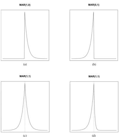
Despite their apparent simplicity and parsimony, MAR models often pro-vide a better fit to economic and financial data as they capture non-linear causal dynamics such as bubbles or asymmetric cycles. The shape of series generated by MAR(r,s) processes depends on the presence of leads, lags and the magnitude of their coefficients. Figure 1 displays how the presence of a lag, a lead, or both, affects the shape of MAR series. Purely causal (resp. noncausal) processes are only affected by a shock after (resp. before) the impact; this is shown in graph (a) (resp. (b)). Consequently, MAR processes are affected both in anticipation and after the shock; the shape of the explosive episode (mostly forward or backward looking) depends on the magnitude of the lag and lead coefficients. When the coefficients are identical (c) the effects of the shock are symmetric around the impact while when the coefficient of the lead is higher (d), the explosive episode is more analogous to what we refer to as a bubble with an asymmetry around the peak.

Figure 1: Effects of lags and leads on a MAR(1,1) series (a) φ = 0.8 and ψ = 0, (b) φ = 0 and ψ = 0.8, (c) φ = 0.8 and ψ = 0.8, (d) φ= 0.3 and ψ= 0.8

autocovariance functions are identical. Fitting an autoregressive model by OLS allows however to estimate the sum of leads and lags,p.3 _{Subsequently,} the respective numbers of lags (r) and leads (s), such that r+s= p, can be estimated by an approximate maximum likelihood (hereafter AML) ap-proach (Lanne and Saikkonen, 2011). The selected model is the one max-imising the AML with respect to r, s and all parameters Ω = (Φ,Ψ,Θ), where Φ = (φ1, . . . , φr), Ψ = (ψ1, . . . , ψs) and Θ is the errors distribution

parameters, such as the scale or location for instance. The AML estimator is defined as follows,

ˆ

Φ,Ψ,ˆ Θˆ=argmaxΦ,Ψ,Θ

T−s

X

t=r+1 ln

gΦ(L)Ψ(L−1)yt; Θ

,

where g denotes the pdf of the error term, satisfying the regularity con-ditions (Andrews, Davis, and Breidt, 2006). Lanne and Saikkonen (2011)

3_{A non-Gaussian MLE can give misleading results in a misspecified model (Gouri´eroux}

show that the resulting (local) maximum likelihood estimator is consistent, asymptotically normal and that ( ˆΨ,Φ) and ˆˆ Θ are asymptotically indepen-dent. Since analytic solution of the maximisation problem at hand is not directly available, numerical gradient-based procedures can be employed. Hecq et al. (2016) indicate that in theory, estimatingMAR models is easier for more volatile series since the convergence of the estimator is faster for distributions with fatter tails. They propose an alternative way to obtain the standard errors, a method implemented in the R package MARX.

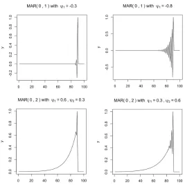
While with a unique lead and a positive coefficientψ, explosive episodes in-crease at a fixed rateψ−1until the crash, other specifications induce complex patterns not resembling the bubble pattern that this paper focuses on. As shown in Figure 2, a negative coefficient (upper graphs) creates increasing oscillations around zero until the crash and multiple leads (bottom graphs) create oscillations along the explosion. Because the presence of multiple leads renders derivations rather intricate, this paper focuses on MAR(r,1) processes with a positive lead coefficient. Except for the empirical analysis of Section 5, the data generating process will be assumed correctly identified throughout the paper to disregard estimation uncertainty.

3

Predictions using closed-form expressions

When it comes to forecasting MAR models, different approaches are avail-able. One can predict the next points of the series based on conditional expectations. Alternatively, one can forecast densities, with for instance the aim to visually analyse probabilities of potential future paths or to predict probabilities of turning point in an explosive episode. However, the antici-pative aspect ofMARmodels complicates their use for predictions. Results are not as straightforward as they could be with purely backward-looking ARMA models. While in some cases mean or density forecasts can be di-rectly obtained from the assumed errors distribution, they sometimes need to be approximated. For this section, let us assume that the data generating process is an MAR(r,1) process Φ(L)(1−ψL−1)yt =εt, where ψ >0, εt is

i.i.d. non-Gaussian andut= Φ(L)ytis the purely non-causal component of

Figure 2: Complex dynamics induced in MAR(0,s) processes by negative coefficients or multiple leads

3.1 Point predictions

Gouri´eroux and Zako¨ıan (2017) derive the first two conditional moments of MAR(0,1) processes,4 here denoted as ut, and show that for Cauchy

processes, withψ >0, the conditional expectation of uT+1 is

EuT+1|uT] =uT. (3)

This result is puzzling since the conditional expectation of a noncausal pro-cess has a unit root even though the propro-cess is stationary. More generally, the conditional expectation ofMAR(r,1) processes,

EyT+1|yT

=φ1yT +· · ·+φryT−r+1+uT,

4

and using Equation (1), is equivalent to

EyT+1|yT

=φ1yT +· · ·+φryT−r+1+yT +φ1yT−1+· · ·+φryT−r

=yT + (1−L)(φ1yT +· · ·+φryT−r+1).

The last equality corroborates the findings of Fries and Zako¨ıan (2019) for MAR(r,1) Cauchy models. They show that the conditional expectation at any forecast horizon for any symmetric α−stable distributed MAR(r,1) process can be expressed as a lag polynomial of the last observed value (see Proposition 3.2 (Fries and Zako¨ıan, 2019)),

EyT+h|yT

=Ph(L)yT,

with h ≥ 1 and where Ph(L) is a polynomial of degree r. Fries (2018)

expanded those results to any admissible parametrisation of the tail and asymmetry parameters ofα-stable distributions and derives up to the fourth conditional moments. He also derives the limiting distribution of those four moments when the variable of interest diverges. He shows that during an explosive episode, the computation of those moments gets considerably sim-plified and are characteristic of a weighted Bernoulli distribution charging probability ψαh _{to the value ψ}−h_u

T and (1−ψαh) to value zero, for a tail

parameter 0< α <2. Those results indicate that along a bubble, the pro-cess can only either keep on increasing with fixed rate or drop to zero. For Cauchy-distributed errors (α = 1), the mean forecast during an explosive episode remains equal to Equation (3), yet for other α-stable distributions the conditional expectation may be drastically simplified. Hence, during an explosive episode, the point forecast of an MAR(0,1) process is a weighted average of the crash and further increase (e.g. a random walk for Cauchy-distributed processes), which can be rather misleading. Density forecasts may therefore be more informative as they carry more information.

3.2 Density predictions

The equivalence of information sets (y1, . . . , yT, yT∗+1, . . . , y∗T+h) and

(v1, . . . , vr, εr+1, . . . , εT−1, uT, u∗T+1, . . . , u∗T+h), where vt = Φ(L)−1εt and

ut = (1−ψL−1)−1εt, allows to predict future values of y from

predic-tions of the forward-looking component of ε, namely u. The asterisk in-dicates unrealised values of the random variables. Most prediction meth-ods hence aim attention at purely noncausal processes – here ut.

Gouri´eroux and Jasiak, 2016) or the causal transition distribution (as named by Gouri´eroux and Zako¨ıan, 2017) of theh future values, (u∗

T+1, . . . , u∗T+h),

given the information known at timeT is as follows,

l(u∗_T+1, . . . , u∗_T+h|y1, . . . , yT)

=l(u∗_T+1, . . . , u∗_T+h|v1, . . . , vr, εr+1, . . . , εT−1, uT)

=l(u∗_T+1, . . . , u∗_T+h|uT),

(4)

where l denotes densities associated with the noncausal process ut. The

reduction of the conditional information set stems from information sets equivalence and the independence between error components. While the interest is on predicting the future given present and past information, it is only possible, by the model definition, to derive the density of a point conditional on its future point. Bayes’ rule is first used to get rid of the conditioning on the present point and a second time to condition on the last point of the forecast. Then, the theorem is applied repeatedly on the first term until the density of all points is conditional on future ones. The conditionalpdf in (4) can thus be expressed as follows,

l(u∗_T+1, . . . , u∗_T+h|uT)

= l(uT, u

∗

T+1, . . . , u∗T+h−1, u∗T+h)

l(uT)

=l(uT, u∗T+1, . . . , u∗T+h−1|u∗T+h)×

l(u∗_T+h) l(uT)

=

l(uT|u∗T+1, . . . , u∗T+h)l(u∗T+1|u∗T+2, . . . , u∗T+h). . . l(u∗T+h−1|u∗T+h)

× l(u

∗ T+h)

l(uT)

.

Equation (2) states that εt = ut −ψut+1, hence, for all t, only ut+1 is necessary to derive ut. Furthermore, given ut+1, the conditional density of ut (which we do not know) is equivalent to the density of εt (which we

know) evaluated at the pointut−ψut+1.5 That is, for any assumed errors distributiong we have,

5_Since

uτ =ψuτ+1+ετ for any time point 1≤τ≤T,luτ|uτ+1(u|x) =gετ(u−ψx) for

all time pointτ and valuesuandx. For simplicity, the density distributions related tout

l(u∗_T+1, . . . , u∗_T+h|uT)

=nl(uT|u∗T+1)l(u∗T+1|uT∗+2). . . l(u∗T+h−1|u∗T+h)

o ×l(u

∗ T+h)

l(uT)

=g(uT −ψu∗T+1). . . g(uT∗+h−1−ψu∗T+h)×

l(u∗_T+h) l(uT)

.

Problems may however arise with the two remaining marginal pdf l(uT)

and l(u∗_T+h). We know that ut=ψut+1+εt=P∞i=0ψiεt+i but the pdf of

a linear combinations of errors may not admit closed-form expressions for some distributions.

For instance, Gouri´eroux and Zako¨ıan (2013) present closed-form solutions for the predictive conditional density of purely noncausal MAR(0,1) pro-cesses with Cauchy-distributed errors. They show that the characteristic function of the infinite sum corresponds to that of a Cauchy with scale pa-rameter _(1−|ψ|γ ₎, where γ is the scale of the distribution of the errors εt.

Hence, in theMAR(r,1) case with Cauchy errors, ut∼Cauchy

0,_(1−|ψ|γ ₎. The predictive density of the purely noncausal process (ut) can thus be

computed as such,

l(u∗_T+1, . . . , u∗_T+h|uT)

=g(uT −ψu∗T+1). . . g(uT∗+h−1−ψu∗T+h)×

l(u∗_T+h) l(uT)

= 1 (πγ)h

1

1 +(uT−ψu∗_T+1)2

γ2

. . . 1 1 +(u

∗

T+h−1−ψu∗T+h)2

γ2

!

× γ

2_{+ (1− |ψ|)}2_u2

T

γ2_{+ (1− |ψ|)}2_(u∗ T+h)2

.

Analogously, sinceuT =ψhu∗_T+h+Pih−=01ψiεT+i, it follows thatuT|u∗_T+h ∼

Cauchy0, γh

, where γh = Ph−i=01|ψi|γ. Hence, for Cauchy distributed errors, instead of theh-dimensional conditional joint density, the conditional density of an h-step ahead point forecast can be obtain as such,

l(u∗_T+h|uT) =l(uT|u∗T+h)×

l(u∗_T+h) l(uT)

= 1 πγh

γ2

h

(uT −ψhu∗T+h)2+γh2

× γ

2_{+ (1− |ψ|)}2_u2

T

γ2_{+ (1− |ψ|)}2_(u∗ T+h)2

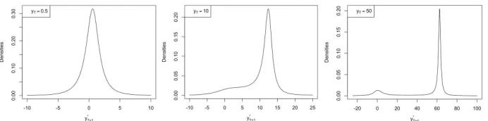
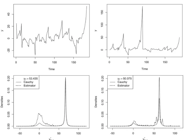
To illustrate how the predictive density evolves as the series diverges, Figure 3 shows one-step ahead forecasts for different levels (yT = {0.50,10,50}))

of a purely noncausal process with a lead coefficient of 0.8 and standard Cauchy-distributed errors. While the predictive distribution is uni-modal for low levels (close to zero), it splits and becomes a bi-modal distribution as the level of the series increases, and the more it diverges the more evident is the bi-modality of the distribution. The two modes correspond to a drop to 0 and a continuous increase to (1/0.8)uT; each event has

probability 0.2 and 0.8 respectively. For instance, when the series attains 50, the probability that it will keep on increasing to a point close to 62.5 is 0.8. Those results corroborate what Fries (2018) shows for diverging Cauchy-distributed MAR(0,1) series. Note that results are analogous for any parameters.

Figure 3: Evolution of the 1-step ahead predictive density as the level of the series increases for anMAR(0,1) with ψ= 0.8.

The predictive density of the purely noncausal filtration of the errors, u, needs to be transformed into that of the variable of interest, y. As ex-plained before, due to equivalence of information sets, the density for (u∗_T+1, . . . , u∗_T+h) can directly be converted into the predictive density of (y∗

T+1, . . . , y∗T+h). In caseytis a purely noncausal process, it is equal to the

processut, and forecasting one is equivalent to forecasting the other.

How-ever, in theMAR(r,1), sincey_T∗₊₁=φ1yT+...+φryT−r+1+u∗T+1, the density of the purely noncausal process is shifted byφ1yT+...+φryT−r+1. Forh= 2, y∗_T+2depends onu∗_T+2 andy_T∗₊₁, which itself depends onu∗_T+1. Overall, the predictive density ofy_T∗_+h (or of the future path of length h) is determined by theh-dimensional conditional joint density of (u∗

T+1, . . . , u∗T+h). Another

predictive density ofh future y’s could be obtained as follows,

l(y∗_T+1, . . . , y_T∗_+h|yT) =

1 (πγ)h

× 1

1 +(uT−ψ(yT∗+1−φyT)) 2

γ2

. . . 1

1 +(y∗T+h−1−φy∗T+h−2)−ψ(y∗T+h−φy∗T+h−1)) 2

γ2

× γ

2_{+ (1− |ψ|)}2_u2

T

γ2_{+ (1− |ψ|)}2_(y∗

T+h−φyT∗+h−1)2 .

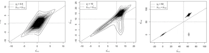
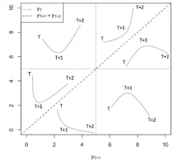
Figure 4 shows the evolution of two-step ahead forecasts of a purely noncausal process with lead coefficient 0.8 and Cauchy-distributed errors as the variable increases. For high levels of the series, the split of the distribution is evident; at each step the series can either keep on increasing or drop to zero, where the latter corresponds to an absorbing state. The interpretation of each area of the graph is explained in Figure 5, showing which region of the graph corresponds to which potential future shape of the series given the last observed point.

Figure 4: Evolution of the 2-step ahead joint predictive density as the level of the series increases for anMAR(0,1) withψ= 0.8 and Cauchy-distributed errors

Figure 5: Future patterns based on joint predictive density. The dotted lines correspond to the last observed point and the diagonal dashed line to the line y∗_T+1=y∗_T+2.

constant |ψ|αh _{for given a given horizon h ≥ 1. This may however not be}

very realistic when it comes to real life data. We might expect probabilities of a crash in stock prices for instant to increase with the level of prices since a bubble cannot go on forever. This reason and the fact that the use of other fat-tail distributions (e.g. Student’s t) may lead to the absence of closed-form expressions for the conditional moments and densities led to the elaboration of approximation methods. The next Section presents two approaches to approximate the conditional densities; the first one uses sample-counterparts (Gouri´eroux and Jasiak, 2016) and the second is based on simulations (Lanne et al., 2012).

4

Predictions using approximation methods

4.1 Predictions using sample-based approximations

This section is based on the approach proposed by Gouri´eroux and Jasiak (2016). They derive a sample-based estimator of the predictive densities based on past values of the series and this method can be applied to any non-Gaussian distribution.

Recall that the predictive density ofh future values (u∗

T+1, . . . , u∗T+h) of an

MAR(0,1) process is as follows,

l(u∗_T+1, . . . , u∗_T+h|uT) =

g(uT −ψu∗T+1). . . g(u∗T+h−1−ψu∗T+h)×

l(u∗ T+h)

l(uT)

One of the reason leading to the derivation of this sample-based estimator is that for some distributions, the marginal distribution ofuT andu∗T+h do

not admit closed-form expressions. They can however, based on the iterated expectation theorem, be expressed as follows,

l(uτ) =Eτ+1l(uτ|uτ+1)

,

with τ = {T, T +h}. Once again the noncausal relationship described in Equation (2) is used to evaluate the conditional distribution of l(uτ|uτ+1)

with the distribution of the errors, g(uτ −ψuτ+1). Subsequently, the ex-pected value of the latter can be approximated by its sample-based coun-terparts as the average obtained using all points from the sample for the conditional variable,

l(uτ) =Eτ+1g(uτ−ψuτ+1)≈ 1 T

T

X

t=1

n

g(uτ−ψut)

o

. (6)

Hence, the predictive density for the MAR(0,1) process ut can be

approxi-mated by plugging the sample counterparts (6) in (5),

l(u∗_T+1, . . . , u∗_T+h|uT)

≈g(uT −ψu∗T+1). . . g(uT∗+h−1−ψu∗T+h)

PT

t=1g(u∗T+h−ψut)

PT

t=1g(uT −ψut)

.

For centred Cauchy- or Student’s t-distributed errors for instance, the density g(uτ −ψut), with τ = {T, T +h}, is maximised when uτ = ψut,

for some 1 ≤ t ≤ T. That is, as uτ departs from all past realised values

of the series, _T1 PT

t=1g(uτ −ψut) will tend to zero. Hence, the estimated

ratio may significantly differ from l(u∗T+h)

l(uT) due to approximation errors

and since the denominator approaches zero when the last observed point departs from all past values, approximations errors of the whole ratio will be amplified for high values of uT. Furthermore, since at time T uT is

Computations for MAR(r,1) processes depend on the last r observed values of y and on uT, and this dependence makes it more difficult to

generalise results. Hence, for the sake of simplicity and comparison, we consider MAR(0,1) processes with a lead coefficient of 0.8 and standard Cauchy-distributed errors. For low levels of the series, results are similar between closed-form and sample-based predictions, regardless of past behaviours. As shown in Figure 6, when the series is close to zero, the sample-based estimator fully recovers closed-form results but as expected, when the series departs from central values distortions appear. Nonetheless, the estimator captures the split of the density and thus the potential outset of an explosive episode.

Figure 6: 1-step ahead forecasts of anMAR(0,1) series with lead coefficient ψ= 0.8 at 2 arbitrary low levels (0.65 and 10.66).

the predictive density. To compute cumulative probabilities, we arbitrarily chose the last observed value as the threshold to obtain probabilities of a decrease. For the two series, probabilities of a decrease are respectively 0.57 and 0.33 compared to the closed-form Cauchy-derived result of approximately 0.23.6 _{Note that the choice of threshold may significantly} affect the outcome as probabilities of a decrease may be significantly larger than probabilities of a drop of at least 20% for instance. This is due to large probabilities assigned to points of similar magnitude to the last observed value. The difference between the sample-based probabilities of the two processes arise from the learning mechanism of this approach. On the other hand, differences between closed-form and sample-based results stem from realised values inducing higher probabilities of following similar paths as before in the approximation method. Those approximation errors can however be considered as updates of probabilities based on what previously happened in the series. If statistically they are approximations errors, in real life, series may tend to behave similarly as in the past and in such case, using only past values instead of all potential values in the estimation of the densities may capture this phenomenon.

Results are similar for two-step ahead predictions; the estimated densi-ties depend both on past behaviours and level of the series. However, predictions with this approach are significantly computationally heavier and if the variable follows an explosive path, precise forecasts of more than two steps ahead are laboriously obtained. Gouri´eroux and Jasiak (2016) propose a method to tackle this issue by elaborating a Sampling Importance Resampling (SIR) algorithm. The algorithm aims at recovering a predictive density based on simulations from a misspecified instrumental model from which it is easier to simulate. They suggest using a Gaussian AR model of order s (here an AR(1)) to simulate the process ut. This

approach recovers the intended densities for low levels of the series but fails to recover both the parts corresponding to the crash and to the increase when the variable exceeds some threshold. This threshold depends on past behaviours and on the underlying distribution, but this failure of the algorithm for high levels of the series stems from the intention to recover a bi-modal distribution from a uni-modal distribution. If the variance of the uni-modal instrumental distribution is not large enough

6

The closed-form result slightly departs from the limiting results of Fries (2018) due to the choice of threshold used to compute the cumulative probabilities (uT). It may be

Figure 7: 1-step ahead forecasts of twoMAR(0,1) series with lead coefficient ψ= 0.8 at an arbitrary level (around 50).

to cover both modes of the sample-based density, the algorithm will not be able to recover the whole conditional distribution. The shape of the Normal distribution significantly depends on past behaviours of the series since the variance is estimated as the variance of the residuals of the MAR model. Hence, for more volatile series, the variance of the instrumental Normal distribution will be larger, yet, as the variable increases and the two modes diverge, there will always be a point from which the SIR algorithm does not succeed in recovering the density anymore.

Cauchy. A limitation is that when closed-form results are not available, we cannot disentangle how much of the derived probabilities are induced by the underlying distribution and how much by past behaviours. An alternative approximation method was proposed by Lanne et al. (2012) and it is based on simulations rather than past points.

4.2 Predictions using simulations-based approximations

Lanne et al. (2012) base their methodology on the fact that the noncausal component of the errors, u, can be expressed as an infinite sum of future errors, which in theMAR(r,1) case is easily obtained as such,

ut= Ψ(L−1)−1εt= ∞

X

i=0

ψiεt+i.

Since stationarity is assumed, the sequence (ψi_{) is converging to zero. Hence,}

they assumed that there exists an integerM large enough so that any future point of the noncausal component of the errors can be approximated as the following finite sum,

u∗_T+h ≈

M−h

X

i=0

ψiε∗_T+h+i, (7)

for any h≥1.

As shown before, any point forecasty∗

T+h depends on the sequence forecast

(u∗_T+1, . . . , u∗_T+h). Using the companion form of an MAR(r,1) model, y∗_T+h can be expressed as the sum of a known component and thehfuture values of ut, where the latter, based on Equation (7), can be approximated as a

linear combination ofM future errors

y_T∗_+h =ι′ΦhyT + h−1

X

i=0

ι′Φiιu∗_T+h−i

≈ι′ΦhyT + h−1

X

i=0 ι′Φiι

M−h+i

X

j=0

ψjε∗_T+h−i+j,

where

yT =

     yT

yT−1 .. . yT−r+1

    

, Φ=

      

φ1 φ2 . . . φr

1 0 . . . 0 0 1 0 . . . 0 ..

. . .. ... ... ... 0 . . . 0 1 0

      

(r×r) and ι=

     1 0 .. . 0     

(r×1).

Thus, forecasting any future pointy_T∗_+h or the path (y∗_T+1, . . . , y_T∗_+h), with h≥1, requires forecasting the sequence ofM future errors (ε∗_T+1, . . . , ε∗_T+M) which we will denote asε∗

+. The issue is that theM-dimensional conditional distribution of ε∗₊ is almost impossible to obtain. Instead, Lanne et al. (2012) propose a way to obtain point and cumulative density forecasts. While the estimation approach they propose (Lanne and Saikkonen, 2011) requires finite variance for the errors distribution, this restriction is not necessary for their forecasting method.

Let g(ε∗

+|uT) be the conditional joint distribution of the M future errors,

which, using Bayes’ rule can be expressed as follows,

g(ε∗₊|uT) =

l(uT|ε∗+) l(uT)

g(ε∗₊).

Thus, for any functionq,

Ehq(ε∗₊) u_T

i

=

Z

q(ε∗₊)g(ε∗₊|uT)dε∗+

= 1 l(uT)

Z

q(ε∗₊)l(uT|ε∗+)g(ε∗+)dε∗+

= E

h

q(ε∗₊)l(uT|ε∗+)

i

l(uT)

.

(9)

Similarly as before,l(uT|ε∗+) can be obtained from the errors distribution g. Yet, since it is conditional on ε∗

+ instead of u∗T+1, we can only obtain the following approximation,

l uT|ε∗+

≈g uT − M

X

i=1

ψiε∗_T+i

!

.

Using this approximation and the Iterated Expectation theorem, the marginal distribution ofuT can be approximated as follows,

l(uT) =ET+1l(uT|ε∗+)

≈E

"

g uT − M

X

i=1 ψi_ε∗

T+i

!#

Overall, by plugging the aforementioned approximations in (9), we obtain

Ehq(ε∗₊) u_T

i ≈

E

"

q(ε∗₊)guT −PMi=1ψiε∗T+i

#

E

"

guT −PMi=1ψiε∗T+i

# .

While Gouri´eroux and Jasiak (2016) use past sample to estimate the en-tity of interest, Lanne et al. (2012) make use of simulations. Let ε∗₊(j) =

ε_T∗(₊₁j), . . . , ε_T∗(₊j)_M, with 1≤j≤N, be the j-th simulated series ofM inde-pendent errors. Assuming that the number of simulationsN is large enough, the conditional expectation of interest can be approximated as follows,

Ehq(ε∗₊) u_T

i ≈

N−1PN

j=1q

ε∗₊(j)guT −PMi=1ψiε

∗(j)

T+i

N−1PN

j=1g

uT −PMi=1ψiε

∗(j)

T+i

. (10)

From (8), we can obtain conditional cumulative probabilities as follows,

Py_T∗_+h ≤x u_T

=Eh1 y∗_T+h≤x u_T

i

≈E

"

1 ι′ΦhyT + h−1

X

i=0 ι′Φiι

M−h+i

X

j=0

ψjε∗_T+h−i+j ≤x

! uT #

That is, for any MAR(r,1) process and for any forecast horizon h ≥ 1, choosing q(ε∗

+) = 1

Ph−1

i=0 ι′Φiι

PM−h+i

j=0 ψjε∗T+h−i+j ≤xu

in (10), where xu = x−ι′ΦhyT, will provide an approximation of P yT∗+h ≤ x|uT

. By computing its value for all possible x we can obtain the whole conditional cdf ofy_T∗_+h.

For the sake of simplicity and comparison, we again consider MAR(0,1) processes with a lead coefficient of 0.8 and Cauchy-distributed errors. Probability forecasts are performed for different levels ofuT; the levels were

u_T Cauchy Simulations-based predictive probabilities

10,000 simulations

50,000 simulations

100,000 simulations

10 0.320 0.322 0.322 0.322 (0.011) (0.005) (0.003)

25 0.259 0.260 0.259 0.259 (0.019) (0.009) (0.006)

50 0.231 0.235 0.231 0.231 (0.036) (0.015) (0.011)

100 0.215 0.238 0.221 0.218 (0.075) (0.028) (0.019)

200 0.208 0.278 0.226 0.217 (0.168) (0.062) (0.040)

Table 1: Probabilities of a decrease computed for different levels of an MAR(0,1) series with lead coefficient ψ = 0.8, derived from closed-form results and from simulations-based approximations. For the latter, mean and standard deviation (in brackets) over 1,000 iterations are reported.

different number of simulations N = {10,000, 50,000, 100,000}, including the 10,000 suggested by Lanne et al. (2012).

may give completely opposite results. Recall that a bubble is triggered by an extreme value, and the date at which this extreme value is attained is the date of the crash. Consequently, if we are investigating an explo-sive episode there must be an extreme value in future points triggering the current explosion. However, as we have seen before, only extreme values at ε∗

T+i inducing the natural rate of increase (1/ψ)i are assigned

significant probabilities. The simulations-based approach will therefore tend to indicate high probabilities of a crash, even with a significantly large number of simulations, if no such values are simulated. However, increasing the number of simulations reduces this discrepancy and brings the mean closer to closed-form results for all levels. Yet, even with 100,000 simulations, standard deviations remain quite large for high levels of the series and this indicates that more simulations are necessary. Overall, the higher the level of the series, the higher should the number of simulations be.

this interval.

Figure 8: Simulations-based predictive cdf’s evaluated at yT = 100 with

different number of simulations compared to closed-form results.

For Student’s t-distributions, while predictions cannot be compared to closed-form results, they are analogous; probabilities converge as the number of simulations is increased. The stability between iterations depends both on the distribution and amplitude of the series but with a large enough number of simulations, they seem to be a good approximation of closed-form results. Overall, once the series follows an explosive path, the number of simulations within the estimator needs to be increased.

5

Empirical Analysis

seem satisfactory from the graphs of the data. It might also well be that the series is stationary around a shift in mean. Hencic and Gouri´eroux (2015) use a cubic deterministic trend for isolating the bubble in the Bitcoin. In order to preserve the bubble features of the data and to obtain a stationary series with locally explosive episodes (that would disappear by taking the returns) we have instead considered the Hodrick-Prescott filtering approach. The detrended series is reported in Figure 9. We are of course aware that this first step might alter the dynamics of the series, probably in the same manner that a X-11 seasonal filter modifies MAR models (see Hecq, Telg, and Lieb, 2017). We leave this important issue for further research. We first estimate an autoregressive model by OLS on the whole HP-detrended Nickel price series. Information criteria (AIC,BIC and HQ) all pick up a pseudo lag length ofp= 2. The three possibleMAR(r,s) specifications are consequently a MAR(2,0), a MAR(1,1) or a MAR(0,2). Using the MARX package a MAR(1,1) with a t-distribution with a degree of freedom of 1.34 and a scale parameter of 356.147 is favoured. The value of the causal and the noncausal parameters are respectively 0.60 and 0.74. We are consequently in the situation in which the predictive density does not admit closed-form expressions (although not very far from the Cauchy), hence the sample- and simulations-based approaches can be used.

Figure 9: HP-detrended nickel prices series. The diamonds represent points from which one-step ahead forecasts are performed in this analysis.

in the predictions but both methods use the information carried by the series until the point of the forecast in the estimation.

The model estimated at the outset of the bubble (point 1) is mostly back-ward looking, the lag coefficient is 0.201 larger than the lead coefficient. However, as we move along the bubble, and therefore add higher points in the estimation, identification tends to favour more forward looking models. There seems to be a structural change in the series between the consecutive points 3 and 4 (between February and March 2007) where the scale suddenly increases by more than 20 and where magnitudes of lag and lead coefficients invert so that the series becomes mostly forward-looking. Furthermore, the degrees of freedom of thet-distribution vary between 1.41 and 1.54 before the crash and decrease to 1.18 once the crash is included in the estimation, implying higher probabilities of extreme events.

Point Model estimated Probability of a decrease

φ ψ t(λ,σ) Sample-based Simulations-based Difference 1 0.763 0.562 t(1.54,259.2) 0.444 0.341 0.103 2 0.758 0.572 t(1.43,258.7) 0.607 0.490 0.117 3 0.748 0.606 t(1.41,257.6) 0.645 0.487 0.158 4 0.573 0.756 t(1.53,281.1) 0.593 0.347 0.246 5 0.571 0.765 t(1.49,280.4) 0.600 0.336 0.264 6 0.677 0.689 t(1.18,289.5) 0.275 0.305 -0.030

Table 2: Models estimated at the 6 distinct points in calendar order, where φ and ψ are the causal and noncausal coefficients respectively and λ and σ the degrees of freedom and scale of the distribution. The corresponding probabilities of decrease at an horizon of 1 computed from the sample- and simulations-based approaches and the difference between them is reported in the last column.

(2016), which furthermore incorporates all past realised values of the series. The difference between them, reported in the last column, represents how much of the sample-based probabilities was induced by the learning mechanism of this approach. We see that as we move along the explosive episode, the difference in probabilities between the two methods increases; this is mostly due to the fact that we get further away from past maximum levels of the series and the sample-based approach, based on its learning mechanism, predict higher probabilities of decrease than the underlying distribution suggests. Probabilities of a crash are the highest at points 2 and 3 due to the identified models, a lower lead coefficient imply higher probabilities of a decrease. At point 1, the low probabilities are due to the relatively low level of the series and for the sample-based approach also to the fact that it is still close to numerous past values. Once predictions are performed after the bubble (point 6), probabilities of a drop with both methods significantly decrease. This is firstly due to the inclusion of the crash in estimation, which alters parameters (lower degrees of freedom and higher lead coefficient), which induces lower probabilities of a decrease, but also to the learning mechanism of the sample-based approach. Indeed, the series already reached three times this level and it once kept on increasing, thus, probabilities that it drops are now lowered by the main bubble and the probability from the sample-based approach is even 3% lower than the simulation-based prediction.

a decrease significantly increase (from less than 0.45 to around 0.6 along the bubble) and the proportion of the probabilities induced by the learn-ing mechanism also increases with the level of the series (from 0.1 to 0.26 difference). We investigated probabilities of a decrease but any threshold can be chosen. From an investor’s perspective, the probabilities that the series will drop under some fixed threshold or by a certain percentage could also be derived, as well as values at risk or expected shortfall. Figure 10 shows how the choice of threshold may affect final probabilities. Cumula-tive probabilities are computed as the area under the curve on the left of the threshold. In the scenario depicted in Figure 10, probability of a decrease at the top of the bubble (point 5) is equal to 0.6 while probability of a drop of at least 25% is 0.484. The simulations-based probabilities of a decrease of at least 25% is equal to 0.322 compared to 0.336 for the probability of a decrease. That is, as explained before, the sample-based approach is much more sensitive to the choice of threshold and this may significantly alter the conclusions drawn from the results. In this scenario the difference between the two methods is reduced to 0.162. Furthermore, note that the detrending method applied to the series may significantly alter results interpretation. A combination of both the sample- and simulations-based predictive probabili-ties could also be employed, relying on the beliefs regarding how likely is the series to follow similar paths as before. Furthermore, farther horizon could be investigated but this is limited by computationally demanding sample-based approximations. An adaptation of the SIR algorithm proposed by Gouri´eroux and Jasiak (2016) to bi-modal distribution could be considered.

6

Conclusion

This paper analyses and compares in details two approximation methods developed to forecast mixed causal-noncausal autoregressive processes. It focuses on MAR(r,1) processes and aims attention at predictive densities rather than point forecasts as they are more informative, especially in the case of explosive episodes.

The sample-based (Gouri´eroux and Jasiak, 2016) and simulations-based (Lanne et al., 2012) methods are compared to closed-form results using MAR(0,1) processes with a lead coefficient of 0.8 and Cauchy-distributed errors. We focus on one-step ahead forecasts to give a rigorous analysis of how and why they may differ from closed-form results. We find that closed-form and sample-based predictive densities start to differ as the series departs from central values, and the discrepancies increase with the level of the series. The sample-based approach gives time-varying probabilities and depends on how similar the event under investigation is to past events. This approach yields results that are a mixture of probabilities ensuing from the underlying distribution and from past behaviours of the series. On the other hand, simulations-based predictive probabilities are a good approximation of closed-form results obtained with Cauchy-distributed errors, as long as the number of simulations in the approximations is large enough relative to the level of the series. Both methods capture the bi-modality of the conditional distribution as the series diverges from central values, which is an indicator of a potential bubble outset.

References

Andrews, B., Davis, R., and Breidt, J. (2006). Maximum likelihood estima-tion for all-pass time series models. Journal of Multivariate Analysis, 97(7), 1638–1659.

Fries, S. (2018). Conditional moments of anticipativeα-stable markov pro-cesses. arXiv preprint arXiv:1805.05397.

Fries, S., and Zako¨ıan, J.-M. (2019). Mixed causal-noncausal AR processes and the modelling of explosive bubbles. Econometric Theory, 1–37. Gouri´eroux, C., Hencic, A., and Jasiak, J. (2018). Forecast performance in

noncausal MAR(1, 1) processes.

Gouri´eroux, C., and Jasiak, J. (2016). Filtering, prediction and simulation methods for noncausal processes. Journal of Time Series Analysis, 37(3), 405–430.

Gouri´eroux, C., and Jasiak, J. (2018). Misspecification of noncausal order in autoregressive processes. Journal of Econometrics,205(1), 226–248. Gouri´eroux, C., Jasiak, J., and Monfort, A. (2016). Stationary bubble

equilibria in rational expectation models. CREST Working Paper. Paris, France: Centre de Recherche en Economie et Statistique. Gouri´eroux, C., and Zako¨ıan, J.-M. (2013). Explosive bubble modelling by

noncausal process. CREST. Paris, France: Centre de Recherche en Economie et Statistique.

Gouri´eroux, C., and Zako¨ıan, J.-M. (2017). Local explosion modelling by non-causal process. Journal of the Royal Statistical Society: Series B (Statistical Methodology),79(3), 737–756.

Hecq, A., Lieb, L., and Telg, S. (2016). Identification of mixed causal-noncausal models in finite samples. Annals of Economics and Statis-tics/Annales d’ ´Economie et de Statistique(123/124), 307–331.

Hecq, A., Telg, S., and Lieb, L. (2017). Do seasonal adjustments induce noncausal dynamics in inflation rates? Econometrics,5(4), 48. Hencic, A., and Gouri´eroux, C. (2015). Noncausal autoregressive model in

application to bitcoin/ exchange rates. In Econometrics of risk (pp. 17–40). Springer.

Lanne, M., Luoto, J., and Saikkonen, P. (2012). Optimal forecasting of non-causal autoregressive time series.International Journal of Forecasting, 28(3), 623–631.