Munich Personal RePEc Archive
Explaining differences in efficiency. A
meta-study on local government
literature
Aiello, Francesco and Bonanno, Graziella and Capristo, Luigi
Department of Economics, Statistics and Finance “Giovanni
Anania”, University of Calabria, Department of Economics,
Business, Mathematics and Statistics “Bruno de Finetti” (DEAMS)
University of Trieste, Italy, Accenture S.p.A. Capital Market
-Financial Services IGEM, 20154 Milan, Italy
10 June 2018
Online at
https://mpra.ub.uni-muenchen.de/88982/
1
Explaining differences in efficiency.
A meta-study on local government literature
1
Francesco Aiello
a, Graziella Bonanno
b, Luigi Capristo
c[email protected] - [email protected] - [email protected]
aDepartment of Economics, Statistics and Finance “Giovanni Anania”, University of Calabria
I-87036, Arcavacata di Rende (CS), Italy
bDepartment of Economics, Business, Mathematics and Statistics “Bruno de Finetti” (DEAMS) University of Trieste, Italy
c Accenture S.p.A. Capital Market - Financial Services IGEM, 20154 Milan, Italy
Abstract This paper reviews the literature on local government efficiency by
meta-reviewing 360 observations retrieved from 54 papers published from 1993 to 2016. The meta-regression is based on a random effect model estimated with the 2-step Random Effects Maximum Likelihood (REML) technique proposed by Gallet and Doucouliagos (2014). Results indicate that the study design matters when estimating a frontier in local government. We find that studies focusing on technical efficiency provide higher efficiency scores than works evaluating cost efficiency. The same applies when using panel data instead of cross-section data. Interestingly, studies that use the Free Disposal Hull (FDH) approach yield, on average, higher efficiency scores than papers employing the Data Envelopment Analysis (DEA) method, thereby suggesting that in this literature the convexity hypothesis of the production set is a matter. Finally, the efficiency of local government increases with the level of development of the analysed countries and is positively related to the national integrity of the legal system. The opposite holds when considering the corruption.
1. Introduction
Efficiency in local government has been a long-standing topic of discussion in economics and has received considerable attention over the last three decades. Two main forces have brought about the great interest in this subject.
First, even though theory clearly explains whether a decision unit is efficient or not (Farrell 1957), controversy has surrounded the empirics of much of the research. This is because the efficiency frontier is unknown and there is no consensus on the superiority of one estimation method over another, as argued by Berger and Humphrey (1997), Coelli and Perelman (1999) and Fethi and Pasourias (2010). The sensitivity of results to model specifications has been addressed in several individual studies which compare the results that different methods (i.e. parametric vs nonparametric) yield from a fixed sample of
municipalities (Athanassopoulos and Triantis, 1998; De Borger and Kerstens, 1996; Geys and Moesen, 2009; Worthington, 2000). Furthermore, the reviews provided by da Cruz and Marques (2014), Narbón‐Perpiñá and De Witte (2018a; 2018b) and Worthington and Dollery (2000) offer valuable arguments in terms of why results differ. However, no study has yet
2
quantified the impact of methodological choices on the variability of efficiency scores in local government.
Second, municipalities face different environmental conditions in terms, for instance, of
social, economic and geographical peculiarities of the “territory” where they operate. It is
argued that these contextual variables are beyond the control of authorities and affect the efficiency of local government, thereby suggesting that any study should control for this heterogeneity (Narbón‐Perpiñá and De Witte, 2018b). Along this line of reasoning, it is also important to highlight that the institutional architecture of many countries has changed rapidly since the 1990s due to extensive deregulation aimed at optimising the use of public resources in offering services of general interest at local level. The institutional reforms accelerate over the last 15 years, thereby increasing the interest in economics and public administration to evaluate the efficiency level and the key-factors influencing the performance of the public sector (Lovell, 2002). Importantly, the institutional framework on how municipalities work differ country-by-country and, therefore, it is reasonable to assume that the heterogeneity in national norms translates into heterogeneity in municipality efficiency.
This said, the main purpose of this paper is to measure the impact of methodological choices and of country-specific factors on the efficiency score variability that we observe in the primary literature of local government. To this end, we perform a meta-regression analysis (henceforth MRA), which is a statistical method that reveals more about a phenomenon that has been studied in a large set of empirical works. By investigating the relationship between the dependent variable (i.e. the efficiency scores of primary studies) and some features of each paper, MRA provides a systematic synthesis of a substantial number of studies and quantifies the role that specific aspects of original papers play in explaining the heterogeneity in results (Glass, 1976; Glass et al., 1981; Stanley, 2001; Stanley and Jarrell, 1989). As Glass (1976, p. 3) states, MRA “connotes a rigorous alternative to the casual, narrative discussions of research studies which typify our attempt to make sense of the
rapidly expanding research literature”. Importantly, by using external information on specific observable country variables for the time and the location that primary papers refer, we provide additional information on how the socio-environmental conditions – e.g. institutions and the development level – impact on the variability of efficiency in local government
(Asatryan and De Witte, 2015; Boetti et al., 2012; Narbón‐Perpiñá and De Witte, 2018a, 2018b; Monkam, 2014).
As in any other survey, the selection of the studies to be meta-reviewed is an important phase of the research. This selection is driven by a set of criteria to be satisfied (cfr. § 2) and tends to cover all the literature without restrictions accruing from the reviewer’s judgements.
This assures that meta-studies suffer less than qualitative reviews from potential bias in reviewing the literature of a specific topic. As will become evident later, this study employs a very large sample of papers, thus ensuring an ample coverage of the primary papers on local government efficiency.
Given the increased interest in MRA in economics and the fact that the literature on local government efficiency lends itself well to being summarised through this approach, it is noteworthy that no exhaustive work has yet provided quantitative evidence about the link between the main features of primary papers and the heterogeneity in results.2 In attempting
3
to fill this gap, this paper uses different MRA specifications and refers to a meta-dataset which comprises 360 observations from 54 papers published between 1996 and 2016 (available in January 2017). In this respect, it is worth noticing that there are two streams of the literature of local government efficiency. Many papers focus on the efficiency of single services provided by local institutions, such as, for instance, public transport (Brons et al., 2005), waste collection (Worthington and Dollery, 2001) or water (Byrnes et al., 2010). An alternative approach is to evaluate the efficiency of municipality in providing any service, thereby addressing the issue from a global perspective (Afonso and Fernandes, 2008; De Borger et al., 1994; De Borger and Kerstens, 1996; Lo Storto, 2013). Our MRA considers the efficiency studies belonging to the literature on the global-services approach.
At this stage of the discussion, it is important to say how we address the issue originating from the fact that the authors propose and publish results that satisfy their expectations and journals tend to publish papers with conclusive evidence. This creates a publication bias, which is relevant in every field of empirical economics and has to be controlled for in any MRA. When the dependent variable of the meta-study is an estimated parameter retrieved from primary regressions, the publication bias is evident and related to the sign and the statistical significance of the estimates. In such a case, MRA scholars control for publication bias by weighting their observations with appropriate measures for the variability of estimates (Bumann et al., 2013; Cipollina and Salvatici, 2010; Doucouliagos and Stanley, 2009; Feld et al., 2013; Stanley, 2008). The publication bias in less apparent in a meta-review of efficiency scores because the dependent variable is not the “estimates of an
effect” (Stanley, 2001, p. 13). This probably explains why this issue is never discussed and controlled for in the previous MRAs on efficiency, with there being the implication that these meta-studies signal to be free of publication bias. However, efficiency scholars have some preferences when estimating a frontier depending on the variability of the estimated scores within the sample. Indeed, whether the efficiency scores exhibit low or high variability around the mean is a matter which influences the assessment of the estimated frontier and, hence, a source of publication bias. Taking into account of this in specifying our meta-regression, we render this paper the first meta-study introducing and controlling for publication bias. The empirical setting we use is based on the 2-step procedure proposed by Gallet and Doucouliagos (2014), the first step of which is based on a random effects model estimated with the REML technique and the second step considers a WLS regression.
Due to its main research focus, i.e. measuring the impact of potential sources of heterogeneity on local government efficiency, this article contributes to the debate assessing the role of methodological choices made by researchers when specifying the frontier of municipalities (see Table S1 of the online supplementary material). Therefore, by applying
MRA to a wide set of observations, the paper’s contribution lies in the fact that we address the
following relevant issues: whether parametric studies yield different results from nonparametric studies; whether DEA studies yield different results than FDH papers; whether the impact differs when considering cost instead of technical efficiency; whether the sample size of primary papers matters in influencing results; whether papers focusing on national municipality provide different efficiency scores than papers focusing on a restricted sub-national geographical area. As these issues refine the identification of the problem to be studied, they address the so-called “apples and oranges” MRA problem, which arises when bringing together studies which are different from one another (Glass et al., 1981). Finally, taking into account the country to which the primary paper refers to, the MRA includes the GDP per capita and two institutional variables relate to corruption and the integrity of legal
4
system. These country-observables are meant to gauge how the context in which the municipalities operate affects the heterogeneity in efficiency.
The paper is structured into six sections. Section 2 describes the criteria adopted to create the meta-dataset, while Section 3 highlights the heterogeneity in efficiency scores. Section 4 presents the MRA and the variables used in regressions. Section 5 presents and discusses the results and Section 6 concludes.
2. The local government efficiency meta-dataset
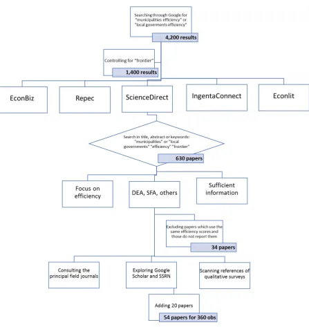
A delicate phase of MRA is the creation of the database. All authors searched, read and coded the research literature. The search was conducted in three phases.
First, we start from Google and have the confirmation that the number of potential material is impressive: for instance, when searching through Google for “local government efficiency”, one obtains more than 102,000 results. Similarly, the search for “local government
studies" yields 195,000 results (as of 31 January 2017). Finally, searching together
“municipalities efficiency” or “local governments efficiency” provides 4200 results. These results comprise a very large sample of documents, thereby making necessary the use of some selecting criteria to handle better the available information within the analytical framework of an MRA. In other words, to collect a representative sample of works, we employed some criteria to identify relevant academic studies from the large pool of papers on the efficiency of municipalities. The filter used browsing Google is “frontier”: adding this to “local government
studies" collapses the search results to 1400 (Figure 1).
Secondly, we referred to the EconBiz, Repec, ScienceDirect, IngentaConnect and Econlit archives. The key words used in the baseline search of titles, abstracts and key words were
“municipalities”, “local government”, “efficiency” and “frontier”. At the beginning, the search was not restricted and provided a sample of 630 published works and working papers encompassing a very broad set of hypotheses and empirical works. Before filtering this sample of works, we ensured that they (a) focused on the efficiency of municipalities when scholars aim at estimating the global rather than the specific-sector performance; (c) included sufficient information to perform the MRA (efficiency scores and standard deviations); (d) ran specific models to estimate the frontier (SFA, DEA, FDH); (e) were written in English; (f) were published in a journal or as working papers. We excluded papers with the same efficiency score results as reported in other papers by the same author(s) and papers that did not report efficiency estimates.
Thirdly, we (a) manually consulted the principal field journals (Journal of Productivity Analysis, European Journal of Operational Research, Local Government Studies, Cities, Omega, Journal of Urban Economics; (b) explored additional databases, such as Google Scholar,
5
Figure 1
The dataset assembling process
3. Does heterogeneity exist in local efficiency literature?
[image:6.595.56.504.147.621.2]6
scale (constant or variable),3 (d) the structure of the data (panel or cross-sectional) and (e)
the data aggregation used in primary papers (regional or national level). Finally, we summarize the efficiency scores retrieved from papers focusing on EU or extra-EU municipalities.
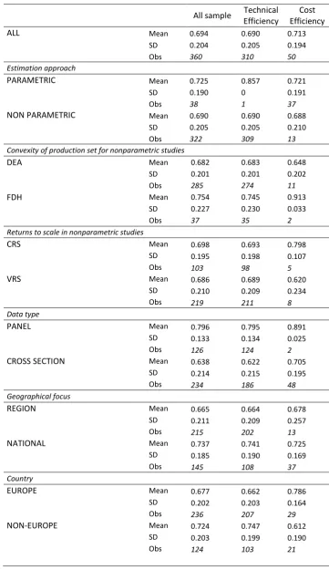
Overall, the sample of 360 observations yields an (un-weighted) average efficiency of 0.694.Some differences emerge by efficiency type: the average of the 50 cost-efficiency scores is 0.713, while it is 0.690 for the 310 observations of efficiency in production.4 The data also
highlight that the overall mean of the 38 observations from parametric studies is higher than that of the 322 observations from nonparametric papers, although the difference in the mean is 0.036(=0.725-0.689) is low and not statistically significant. The sample-size impedes to compare nonparametric and parametric studies for technical efficiency, while the difference remains in favour of parametric methods for papers focusing on cost frontiers.
There are 285 observations referring to DEA studies (274 of which refer to technical efficiency), more than 76% of the entire sample, while the dataset includes 37 observations from studies using FDH approach. As for as the all sample is concerned, it emerges that FDH studies yield higher efficiency scores than DEA papers. The difference in means is high when considering the technical efficiency (unfortunately the meta-dataset comprises only two observations of cost efficiency from FDH papers). With regard to the structure of the data used in primary studies, the analysis shows that about two-thirds of the observations come from estimations obtained from cross-sectional data and the other one-third from panel data. What clearly emerges is that the average of efficiency scores is 0.796 for papers using panel data, that is a value significantly higher than the average (0.638) associated to cross-sectional studies. The same applies for technical efficiency studies.
A pattern to be pointed out is observed when grouping the observations for the hypothesis of returns to scale in nonparametric studies. Overall, the use of variable returns to scale (VRS) translates to an average level of efficiency equal to 0.686, which is slightly lower than that (0.698) associated with observations using the hypothesis of constant returns to scale (CRS). However, the difference is means is not statistically significant. This result is confirmed for the sub-sample of studies estimating the technical efficiency.
Furthermore, in the sample, another difference is that 215 observations refer to papers using data of municipalities belonging to one or more regions of a country and 145 refers to studies covering all the local entities of a country. In other words, there are more papers focusing on how municipalities work in a region than those looking at country level. The evidence shows that the un-weighted average of efficiency scores associated to “regional” studies is 0.664, that is lower than that (0.737) obtained from primary papers covering the national municipality organization. This outcome is found for both sub-sample of observations, that is technical or cost efficiency scores. Finally, we find that papers on European municipalities yield lower efficiency scores than studies analysing the local government of other nations.
3 The list of the studies which make up the meta-dataset is provided in the Table S2 of the online supplementary material. That table includes the authors’ name, the year of publication, the type of publication, the journal, the number of estimates, the average efficiency and some measures of variability (standard deviation, maximum and minimum values). We only display the average for the primary studies reporting different measures of efficiency (i.e. technical or cost efficiency). Nevertheless, the econometric analysis uses all the information from every paper.
7
[image:8.595.88.512.323.656.2]While table 1 reveals that there are differences in mean and a certain variability of efficiency scores, the figure 2 sheds some lights on the entire efficiency distribution. Indeed, it highlights significant differences in shapes and forms of efficiency score distributions when primary papers are grouped by the approach used in estimating the frontier (parametric vs nonparametric, panel a), the method set up in estimations (SFA, DEA and FDH, panel b), the efficiency-type (cost vs technical efficiency, panel c), the data used in the empirical analysis (panel data vs cross-section, panel d), the geographical focus (regional vs national, panel e) and, finally, by distinguishing papers addressing efficiency of European or non-European municipalities (panel f). What clearly emerges from these distributions is that any choice made by researchers may affect final estimations of efficiency. Phrased differently, a lesson learnt from this discussion is that the study design of primary papers plays an important role in determining differences in the means and distributions of local government efficiency scores. Finally, the estimated level of efficiency differs, as expected, country-by-country. This is displayed in figure 3 which also highlights how relevant the intra-country variability is.
Figure 2 Heterogeneity in Local Governments’ Efficiency Literature
0 .2 .4 .6 .8 1
PARAM
NON PARAM
(a) By method
0 .2 .4 .6 .8 1
SFA
FDH
DEA
(b) By method II
0 .2 .4 .6 .8 1
TE
CE
(c) By efficiency type
0 .2 .4 .6 .8 1
PANEL
CROSS SECTION
(d) By data type
0 .2 .4 .6 .8 1
REGIONAL
NATIONAL
(e) By geographical focus
0 .2 .4 .6 .8 1
EUROPE
NON EUROPE
8 Table 1 Average, standard deviation and number of observations in local government
literature, by group (averages are un-weighted)
All sample Technical Efficiency
Cost Efficiency
ALL Mean 0.694 0.690 0.713
SD 0.204 0.205 0.194
Obs 360 310 50
Estimation approach
PARAMETRIC Mean 0.725 0.857 0.721
SD 0.190 0 0.191
Obs 38 1 37
NON PARAMETRIC Mean 0.690 0.690 0.688
SD 0.205 0.205 0.210
Obs 322 309 13
Convexity of production set for nonparametric studies
DEA Mean 0.682 0.683 0.648
SD 0.201 0.201 0.202
Obs 285 274 11
FDH Mean 0.754 0.745 0.913
SD 0.227 0.230 0.033
Obs 37 35 2
Returns to scale in nonparametric studies
CRS Mean 0.698 0.693 0.798
SD 0.195 0.198 0.107
Obs 103 98 5
VRS Mean 0.686 0.689 0.620
SD 0.210 0.209 0.234
Obs 219 211 8
Data type
PANEL Mean 0.796 0.795 0.891
SD 0.133 0.134 0.025
Obs 126 124 2
CROSS SECTION Mean 0.638 0.622 0.705
SD 0.214 0.215 0.195
Obs 234 186 48
Geographical focus
REGION Mean 0.665 0.664 0.678
SD 0.211 0.209 0.257
Obs 215 202 13
NATIONAL Mean 0.737 0.741 0.725
SD 0.185 0.190 0.169
Obs 145 108 37
Country
EUROPE Mean 0.677 0.662 0.786
SD 0.202 0.203 0.164
Obs 236 207 29
NON-EUROPE Mean 0.724 0.747 0.612
SD 0.203 0.199 0.190
9
0 .2 .4 .6 .8 1
Australia Belgium
Brazil
Czech Republic
Germany
Greece
Indonesia Israel
Italy
Japan
Korea Macedonia
Malaysia
Morocco
Portugal
Serbia
Slovenia South Africa
Spain
Taiwan
Turkey
USA
Fi
gu
re 3
. Mea
n
ef
fi
ci
e
n
cy sco
res of
lo
ca
l
gov
ern
men
t by count
[image:10.595.340.716.40.550.2]10
4. Meta-analysis of local government efficiency
Section 3 highlights that variability in the mean efficiency scores is relevant when grouping observations by different criteria. Given this, providing a systematic explanation of the variability in efficiency becomes an important issue to be addressed on econometric grounds. The following sub-section 4.1 presents the meta-studies on efficiency, while sub-sections 4.2 and 4.3 focus on the specification of the meta-regression we use to explain the heterogeneity in efficiency scores of municipalities.
4.1 The MRAs on efficiency studies in a nutshell
Before presenting our MRA, it is of interest to point out that the meta-studies on efficiency have increased over time. This field of research has a groundin the seminal paper by Stanley (2001), where he said that “in a meta-regression analysis, the dependent variable is a
summary statistic, perhaps a regression parameter, drawn from each study, while ….” (p. 13). This statement suggests that MRA is not exclusively on “a regression parameter” and,
therefore, it leaves room to perform MRA not only on “estimates of an effect” (see footnote 1)
but also to detecting why results differ in a particular area of research (on this see also Stanley and Jarrell, 1989). As far as efficiency analyses are concerned, the stylised fact is that there is a huge heterogeneity when collecting the results of primary papers, whatever the sector. Then, it is of value to search for the reasons explaining the actual heterogeneity in the mean of efficiency scores, and in this direction the MRA approach provides valuable insights.
A proof of this is that the MRA applications cover a wide spectrum of topics. For instance, Bravo-Ureta et al. (2007) examine the efficiency scores of 167 farm-level studies published over four decades. Thiam et al. (2001) review 34 articles on agricultural efficiency in developing countries. Another MRA on agriculture is provided by Ogundari (2014) which investigates the dynamics of African agricultural efficiency levels obtained from 442 frontier studies. Djokoto and Gidiglo (2016) and Djokoto et. al (2016) focus on the heterogeneity in efficiency scores from 34 primary papers on Ghanaian agriculture. Iliyasu et al. (2014) aimed at explaining the variability observed in 36 efficiency papers on aquaculture. Fan et al. (2018) review 49 studies with field experimental results in water use efficiency of wheat and cotton. Brons et al. (2005) focus on 45 urban transport studies. Odeck and Bråthen (2012) analyse the efficiency of seaports using 40 published papers. Nguyen and Coelli (2009) focus on hospital efficiency referring to 95 studies published over the period 1987–2008. Similarly, Kiadaliri et al. (2013) provide a systematic review of Iranian hospital efficiency estimated in 29 primary papers. Havránek and Iršová (2010) review 32 efficiency studies – with 53 observations – on banking in the US published in 1977–1997. Banking efficiency is also the theme of the MRA performed by Aiello and Bonanno (2018), who review 120 studies – with 1,661 observations – published over the period 2000–2014. Assaf and Josiassen (2016) meta-review the tourism literature by comparing the efficiency scores of 57 frontier papers. Tian et al. (2012) offer some explanations of productivity growth in China using more than 5,000 point-observations from 150 primary studies. Finally, Simões and Marques (2012) conducted an MRA on 107 studies on efficiency in the waste sector.
What we have learnt is that meta-reviewing the mean efficiency scores is becoming a prominent area of research in economics. After highlighting this, here it is useful to say that
the general “apples and oranges” issue of any MRA (see Introduction) holds in the
11 “means comparing values that consist of a heterogeneity component and an efficiency component” (p. 7).5
By following Brons et al. (2005), let’s assume the existence of a theoretical frontier C
[image:12.595.163.435.444.644.2]with a universal value. The estimated mean efficiency is higher in A than in B, but the real efficiency in sample B is higher than in sample A (figure 4). Hence, taking the mean value of the estimated efficiency, the meta-study does not compare the single point-observations but compares the sample heterogeneity (heterogeneity component). Again, if the specific frontiers are the highest attainable efficiency levels given the study-specific conditions, then the exercise to compare the mean efficiency scores will be a mode to compare the actual efficiency scores (efficiency component) (Brons et al., 2005). MRA takes into account these two components because, on one hand, the study-specific heterogeneity arising from differences in sample composition can be handled by applying an unobserved effects framework (Bron et. al., 2005; Merkel and Holmgren, 2017). In particular, study-specific heterogeneity is treated with individual intercept terms to cope with differences in sample composition (the ui term in our equation [3]). On the other hand, when considering the efficiency component, it is known that in the meta-regression context, the aim is to explain the variation in efficiency scores by using the variation in a number of moderator variables. Therefore, the feasible way to deal with the problem of study comparability is to specify an econometric model in such a way that the within-study variation is used to explain the variation in the efficiency estimations (Brons et al., 2005). In other words, the differences in the efficiency of primary papers (efficiency component) are handled by including the moderator variables in the analysis (Merkel and Holmgren, 2017).
Figure 4 The comparison of mean efficiency from different studies
Source: Brons et al. (2005)
5 The comparability issue is also part of the meta-reviews which do not use meta-regressions. For instance, Pittelkow et al. (2015) selected and compared 678 efficiency studies on no-till agriculture. The role of non-tillage is also meta-reviewed by Zhao et al. (2016) who use evidence from 39 efficiency studies on China. Varabyova and Müller (2016) meta-review 22 efficiency studies on health care production in OECD countries. Finally, Minviel and Latruffe (2017) focus on the effect of public subsidies on farm efficiency.
C
A B
O X
12
4.2 Methodological issues and MRA specification
An important issue to be addressed in this kind of empirical analysis concerns the heteroscedasticity. In our case, the dependent variable of the MRA is the efficiency score of municipalities retrieved from the primary literature. As we have seen above, in creating the meta-dataset we have collected all the information from each paper, and many papers provide more than one estimate of efficiency. From an econometric perspective, this means that the unit of observation is the individual value of the estimated efficiency, with the result that there is within-study heterogeneity to control for. This is done by running a WLS regression, which is part of the second step of the procedure proposed by Gallet and Doucouliagos (2014). An additional check of the clustering issue has been made by implementing the methodological developments proposed by Jackson et al. (2011) and Hedges et al. (2010) (see footnote 7).
There is another issue/concern that should be controlled for in meta-reviewing the literature on a specific topic. We refer to the publication bias originated by the fact the success of a paper depends greatly on the study results in that the probability of a paper being published increases the more conclusive its conclusions. In every meta-study, a simple method for detecting publication bias is to regress the key variable of the meta-analysis – generally a parameter of a primary regression – against its precision in primary estimations
(Egger et al., 1997). If this regression yields significant results, there is evidence of publication bias in the meta-dataset which must be controlled for in the MRA. Something changes when meta-reviewing efficiency scores, as the dependent variable is not a single point estimate which is expected to be significant, but it is the mean value retrieved from an efficiency study. Although the risk of publication bias is less apparent than in the MRA on primary regressions, it continues to exist, as scholars and journals do have some expectations when estimating a frontier. For instance, the frontier is low informative when the efficiency scores are not variant and then scholars prefer a certain degree of variability: they react positively when the variability of the efficiency scores does not tend to zero. The standard deviation of efficiency scores is zero in two cases, the first of which is pointless,6 while the second case occurs when
all the Decision-Making-Units (DMUs) lie on the frontier. In such a case, the efficiency is unity
in mean with zero variability. This frontier has the caveat that no ranking among the DMUs is possible, which, on the contrary, is a value in efficiency studies, so much as different methods to rank efficient/inefficient DMUs are proposed (Adler et al., 2002; Khodabakhshi and Aryavash, 2012). Differently phrased, the efficiency ranking of individual DMU is an important micro application of any frontier analysis and it exists if results are variant. On the other hand, efficiency scholars might be worried whether the study yields some mean efficiency and a huge dispersion covering the range of the [0,1] interval. In such a case, the key questions in evaluating the efficiency results are: Does the frontier specification not properly control for the heterogeneity across DMUs? and/or Could be the sample composed by different groups with different scopes and behaviours, thereby estimating only one frontier has not a sense? However,
a certain degree of variability of efficiency scores is desired because it signals that the reasons for efficiency/inefficiency are heterogeneous. This difference in DMUs behaviour is crucial for adopting solutions to improve their individual performance. In brief, people estimating frontiers expect some variability in the efficiency distribution as either they can detect why the DMUs are inefficiency or provide rank among DMUs.
Based on the above considerations, we have learnt that – compared to the regression primary analyses – here there is no clue about the natural distribution of inefficiency and its
13
parameters (for instance, a reasonable average, standard deviation, type of skew) and much is
left to the researcher’s experience and preferences. From our perspective, this is a certain source of potential publication bias, which has never been discussed and treated in the meta-studies on efficiency (see § 4.1).
This said, in order to provide answers to the research questions raised throughout the paper, we refer to the following equation:
i i S
j j j 0 1i β X
E [1]
where the dependent variable Ei is the i-th efficiency score. Eq. [1] is known as the funnel asymmetry test–precision effect test (FAT-PET) MRA (Stanley 2005, 2008), where Si is a
measure of the variability of Ei, which is the standard deviation of the efficiency scores as
estimated in primary papers. It enters into the meta-regression to control for publication bias. Furthermore, Xj comprises the explanatory variables that summarize various model characteristics of the primary studies. Finally, the error component ε of eq. [1] is clearly heteroscedastic because the efficiency scores have a different variance in the sample and are not independent within the same study. The heteroscedasticity issue is addressed by weighting the observation through a measure S of the variability of each observation of our meta-study: i i i i i i i i e X S E e S S S
j * j * 1 0 * j j j 1 0 i β X β 1 E [2]where the disturbance
e
S
is corrected for heteroscedasticity. The test for publicationbias is carried out on the constant
0, as in Aiello and Bonanno (2018), Bumann et al.(2013), Cipollina and Salvatici (2010), Doucouliagos and Stanley (2009), Egger et al. (1997), Feld et al. (2013) and Stanley (2008).The method used in estimating eq. [2] may be a fixed effects or random effects model. These methods differ in terms of their treatment of heterogeneity. In particular, a fixed effects meta-regression assumes that all the heterogeneity can be explained by the covariates and leads to excessive type I errors when there is residual, or unexplained, heterogeneity (Harbord and Higgins 2008; Higgins and Thompson 2004; Thompson and Sharp 1999). Instead, a random effects meta-regression also allows for such residual heterogeneity (the between-study variance not explained by the covariates) and, therefore, extends the fixed effects model. Formally, under the random-effects framework, eq. [2] becomes:
i i i i
i S X u e
E
j * j * 1 0
* β
[3]
where ei ~ N(0, σ2i) is the disturbance and ui ~ N(0, τ 2) is the primary study fixed effect. The parameter τ2 is the between-study variance, which must be estimated from the data as in Harbord and Higgins (2008).7 To provide some robustness of the results to clustering, we
7 Technically, REML first estimates the between-study variance τ2 and then estimates the coefficients, β, with the weighted least squares procedure and using as weights 1/(σi2 + τ2), where σi2 is the standard deviation of the estimated effect in study i. The term “multilevel” refers to the structure of
14
adopt a two-step procedure as in Gallet and Doucouliagos (2014) and Aiello and Bonanno (2018). An REML regression is run in the first step. Importantly, in the second step we run a WLS regression in which the weights also include the value of τ2 retrieved from the first step. This ensures that the REML estimates will be robust to clustering at the study level.8
4.3 The explanatory variables in the meta-analysis
The right-hand side of eq. [3] includes the matrix Xi, which is related to the observed characteristics used to explain the variability in local government efficiency that we have identified on the basis of a systematic comparison of original papers. The explanatory variables are discussed in the following.
A first group of variables is anchored to the specific topic of the analysis that is the study of heterogeneity in efficiency. Then, a distinguishing element to be considered relates to the approaches and methods used to estimate the frontier. We firstly made a broad distinction between papers using a parametric method and papers following a nonparametric approach. To this end, the dummy variable used is Parametric (PARAM), which is equal to unity for the
first group of studies and zero for the others. Additionally, as we have already pointed out (cf. Introduction), nonparametric papers distinguish between DEA and FDH methods to estimate the frontier. In this respect, after restricting the sample to nonparametric papers we include the dummy FDH, which is unity when efficiency scores are derived from primary studies using
the FDH (the controlling group comprises the point observations from papers using DEA). Furthermore, to control for efficiency type we include the dummy TE, taking the value of 1 if
the primary estimation refers to technical efficiency (the controlling group is the efficiency obtained from the cost frontiers). Finally, there is another factor belonging to this groups that ought to be taken into account,9 which is related to the assumption on returns to scale: in this
also driven by the structure of our data. As our dataset contains high variability in primary studies, the fixed effects estimator is expected not to perform well because it does not allow for between-study variability. Conversely, REML fits our case well. The evidence we find supports the use of the random effects model as the between-study variance is high and significant (cfr. Table 1). This holds
despite the potential caveat of REML, the results of which are reliable if the random effects variance is properly estimated (Oczkowski and Doucouliagos, 2014). Importantly, Stanley and Doucouliagos (2015) compare REML and WLS and their analysis is not conclusive, depending on additional extra heterogeneity and publication bias effects.
8 To address the clustering issue with greater effectiveness, we have also taken into consideration the developments proposed by Jackson et al. (2011) and Hedges et al. (2010). Jackson et al. (2011) claim “the absence of information about the within-study correlation structure does not entirely prohibit a multivariate approach but this does present very real statistical issues and a consensus about the best approach or approaches has yet to be reached” (p. 2495). The model proposed by Hedges et al. (2010) requires knowing the dependence structure within each study. Their routine (the “robumeta” Stata command) runs after assigning a value to the parameter of dependence. This means that on the one hand, we search for a technique yielding robust standard errors and on the other hand, the advances in econometrics assume that the within-study variability is known. In other words, in Hedges et al. (2010) the standard errors are correct if and only if the assumed value of the dependence is valid and there is no way to test this assumption. It is also worth pointing out that the "robumeta" command is not yet for use in research as noted in a message that emerges when launching a regression (“this routine needs to be verified, do not use for research purposes”). Based on
these arguments, we left the within-study issue within the REML framework for future research as it is still an open question in the econometrics of meta-analysis.
9When performing an efficiency study based on parametric methods, researches make another choice
15
respect we consider the dummy variable VRS which is equal to 1 if the primary study assumes
VRS and zero otherwise (the controlling group comprises the point-observations from studies using constant returns to scale, CRS). As parametric studies do not provide any information regarding the returns to scale assumption, we restrict the test to the nonparametric studies.
Secondly, a number of regressors is from the literature on meta-regression which gives some guidance regarding the issue to be addressed in the analysis. A distinction to be made is between the efficiency obtained in papers using cross-sectional data and that derived from studies based on panel data. The dummy variable Panel is equal to unity if the original works
used panel data and zero otherwise. We also control for the time effect by using the Year of publication of the primary paper. Furthermore, we consider the variables lDIM, given by the
sum of the number of inputs and outputs of the frontier (in logs) and lSIZE, which is the
number of observations used in primary papers when estimating the efficiency score. In such a case, we also include the interaction lSIZE*MANY for testing if the sample size has an effect
of the primary estimated efficiency when they refer to a high number of municipalities (MANY
is a binary variable equal to 1 if the number of municipalities is greater than 2000).
Thirdly, our MRA includes the dummy DREG, which distinguishes between the efficiency observations for a specific sample of municipalities belonging to one or specific regions of a country (DREG=1) and observations referring to papers covering all the municipalities of a country (DREG=0). The coefficient of DREG is expected to vary moving from national to sub-national groups of municipalities, although there is no a priori expectation on its sign. The
result depends on the homogeneity of the sample of municipalities used in estimating the frontier: if regional municipalities are homogenous, then the estimated efficiency score will be expected to be higher than that obtained from heterogeneous samples (i.e. all municipalities of a specific country): all else being equal, similar municipalities exhibit similar behaviour and thus are more clustered around a frontier than different municipalities with divergent goals. In addition, to control for geographical differences, we consider the dummy variable Europe,
which are equal to 1 if the study used data from a European country (in estimating the MRA, the controlling group comprises efficiency scores from papers focusing on the rest of the world).
Here, it is worth mentioning that the numerous different ways of performing an efficiency study make conclusive expectations of the impact of each regressor difficult. Indeed, despite the high degree of specialization in the use of various methods, the effect of some methodological choices is still not certain. For example, efficiency in parametric studies may be higher or lower than that obtained in nonparametric papers, depending on the nature of disturbances from the frontier (Nguyen and Coelli 2009). The use of panel data would generate higher efficiency levels than those from cross-sectional data. Finally, efficiency would increase with the number of variables included in the frontier, while it would decrease with small sample sizes and the assumption of CRS (Berger and Humphrey, 1997; Coelli, 1995; Fethi and Pasourias, 2010; Nguyen and Coelli, 2009). However, while theory predicts the likely impact of any choice, the actual measure of how sensitive the results are to the study design is an issue to be addressed empirically.
We insert three country-specific variables.
The first is the GDP per capita of the country analysed in the primary paper. It is retrieved from World Bank database and it is based on purchasing power parity (PPP). Data are in constant 2011 international dollars. Result expectations are mixed. On one side local
However, our MRA disregard this issue because the observations from parametric studies are few (only 38, table 1), thereby limiting the possibility to run a regression. The number of efficiency scores from translog function forms are only 10, the Cobb-Douglas sample comprises 27 observations (10 of which are without standard errors, cfr. § 3). The metadata also contains 1
16
government efficiency would increase with the level of development of the country as higher income citizens pay greater taxes and have more requirements on local services and facilities (Asatryan and De Witte, 2015; Afonso and Fernandes, 2008; Boetti et al., 2012; Ibrahim and Karim, 2004; Kalb et al., 2012). On the other hand, local government is expected to manage higher financial resources in high-income country with a potential reduction of incentives to reach efficiency (Ashworth et al., 2014; Bosch-Roca et al., 2012; Da Cruz and Marques, 2014; De Borger et al., 1994; De Borger and Kerstens, 1996a, 1996b; Monkam, 2014).
The second country observable we use is the Corruption Perceptions Index (CPI) derived from the Transparency International website (https://www.transparency.org/) where 180 countries and territories are ranked by their perceived levels of public sector corruption according to experts and business people. The index uses a scale of 0 to 100, where low values denote high corruption and high values very clean. In 2017, it is found that more than two-thirds of countries score below 50, with an average score of 43. It expected that efficiency in local government is high when the regulatory framework of a country assures transparency and public participation, that is, when the incentives for corrupt behaviour are low (World Bank, 2004). MRA results would provide some evidence whether efficiency studies for countries with high corruption yield results which differ from those obtained when focusing on less corrupted countries.
The third country-specific factor is the Integrity of Legal System (ILS) index retrieved from the annual reports released by the Fraser Institute. As a good legal system is a pre-requisite for economic freedom, the ILS index is meant to gauge any potential links between the economic freedom and the efficiency on how municipalities work. The key ingredients of a legal system consistent with economic freedom are rule of law, an independent and unbiased judiciary, and impartial and effective enforcement of the law. Security of property rights, protected by the rule of law, provides the foundation for both economic freedom and the efficient operation of markets. Freedom to exchange, for example, is fatally weakened if individuals do not have secure rights to property, including the fruits of their labour. When individuals and businesses lack confidence that contracts will be enforced and the fruits of their productive efforts protected, their incentive to engage in productive activity is eroded. All this is essential for the efficient allocation of resources. In other words, an effective legal system would force local authorities to be efficient because of private sector claims for a good public sector (Ammons, 2018; Worthington, 2000). Additionally, there could also be some pressure for productivity improvement in local government because of the perceived threat to job security of civil servants: countries with secure rights to property foster the economic freedom to do business, thereby implying that, all things being equal, some services may be privatised. In such a case, municipalities might react by increasing their efficiency and then retaining the services they offer (Savas, 2018). The aim of MRA is to understand whether the variability in primary results depends on how effectively the protective functions of government are performed.
17
Figure 5 Scatter plots between efficiency scores (y axes), GDP per capita, CPI and ILS, averaged by country*
*Countries are: Australia, Belgium, Brazil, Czech Republic, Germany, Greece, Indonesia, Israel, Italy,
Japan, Korea, Macedonia, Malaysia, Morocco, Portugal, Serbia, Slovenia, South Africa, Spain, Taiwan, Turkey, and USA. Data details at country level are reported in the appendix table A1.
Legend: CPI is the Corruption Perceptions Index; ILS is the Integrity of Legal System index.
5. Fitted models and analysis
5.1 Fitted models and diagnostics
As the underlying idea is to test the robustness of the results (sign, magnitude and significance) when moving from basic to extended regressions, in presenting the results, we start from a regression just including the dummies relating to the regional/national samples of the primary papers (DREG) and to the geographical areas (Europe) which the primary analysis refers to. Results are displayed in Table 2, model 1. Model 2 adds the variables related to the efficiency and data type (TE and PANEL, respectively), the methods (PARAM),
the number of variables (lDIM) and the sample size (lSIZE) used to estimate the efficiency
scores of municipalities in primary studies.10 Finally, we also include the Year of publication.
10The dummy associated with TE enters into the regression not to provide a ranking across efficiency types, but simply to check if the main results hold when controlling for the frontiers to which the single observation refers. Furthermore, the MRA collects observations from very different papers and thus there is no expectation on TE compared to cost efficiency (CE). We can use an example to explain the issue. When estimating a cost frontier with input-oriented technology for a given sample of local governments, say sample A, we know that a municipality is inefficient because its technical and/or allocative efficiency is low. Therefore, for this sample, the cost efficiency, say CEA, is at best equal to the technical efficiency TEA. This ranking TE≥CE is predicted by theory (Kumbhakar and Lovell 2000: 54). However, any empirical outcome is admitted when comparing efficiency scores
.2
.4
.6
.8
1
Mean GDP per capita
(a) Efficiency and GDP per capita
.2
.4
.6
.8
1
M
e
a
n
E
ff
ic
ie
n
c
y
Mean CPI
(b) Efficiency and CPI
.2
.4
.6
.8
1
Mean ILS
18
In model 3, the interaction lSIZE*MANY allows to test the effect of sample size when the
number of municipalities is high.
Table 3 reports the evidence we find for specific sub-samples of observations belonging to the class of nonparametric studies. In this case, we test the convexity hypothesis of the production set in performing a nonparametric efficiency study. To this end, we introduce the dummy FDH, which is equal to 1 when the primary studies relax the convexity
hypothesis (model 4). In addition, we include VRS to control for the heterogeneity depending
on the hypothesis of returns to scale (models 5 and 6). Lastly, we carried out a sensitivity analysis to test whether the evidence is robust to the substitution of the variable Year of publication with the variable Year of estimation, which the primary study refers to (see the
supplementary material).
Before presenting the results, it is worth discussing some diagnostics. The main evidence regardsˆ0, the parameter used as a test for publication bias. If
0
0
(FAT) thenthere will be asymmetry in the estimates and publication selection (Stanley 2005, 2008). ˆ0 is significant in models 1, 2 and 3, but not in models 4, 5 and 6, indicating that when the focus is on nonparametric studies there is no evidence of publication bias in REML regressions with the covariates. The estimation of ˆ0 remains significant when performing the sensitivity analysis (Table S3 of the supplementary material).
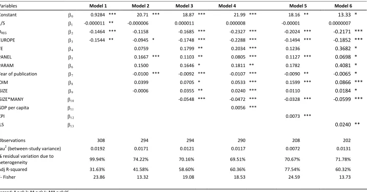
Furthermore, we present some statistics at the bottom of each table that we retrieved from the Stata command “metareg”, developed by Harbord and Higgins (2008). As can be seen, the proportion of the residual variance that is attributable to between-study heterogeneity is very high: in model 1 it is 99.94%. Again, in the same regression, the proportion of between variance explained by the covariates is 31.63%, the measure of within-study sampling variability. When we include additional regressors, between-within-study heterogeneity tends to decrease (in model 3 it is equal to 70.19%), while the proportion of between variance explained by the covariates tends to increase (in model 3 it becomes 58.60%). Finally, the joint significance of the explanatory variables is high in each model. To ensure clarity in the presentation of the results, the discussion is divided into three sub-sections. The first is devoted to the role of data aggregation and geographical context. The second sub-section focuses on the estimating methods, while the third looks at the effects exerted by the features and the study-design of primary-papers.
5.2 Data aggregation and geographical context
Estimations referring to a specific region of a nation yield lower efficiency scores on average respect to estimations made on all the municipalities of a country. This holds for all the estimated models. The parameter
ˆ2 associated to dummy DREG ranges between -0.25 inmodel 6 to -0.15 in model 1 (the lowest value is estimated in model 2, but only in this case
ˆ2 results not significant). The implication of this evidence may be useful for scholars, as one may expect a lower level of efficiency when focusing on sub-national areas (the municipalities
19
of a region/province)11 than when addressing the efficiency issue by considering all
municipalities of a country. We also find that studies focusing on municipalities of European countries yield on average lower efficiency scores than papers that analyse the local government of other nations. Indeed, the parameter
ˆ
3 associated to dummy EUROPEassumes values between -0.24 (model 6) and -0.09 (model 2).
5.3 The role of estimating methods
Regarding the methods used to estimate efficiency in primary papers, we find that the coefficient associated to dummy PARAM is significant and positive (
ˆ
6
0
.
16
) in model 2 oftable 2. This also occurs in the sensitivity analysis, as
ˆ
6
0
.
13
is model 1, while
ˆ
6
0
.
15
in model 2 of table S3 of the online supplementary material. The conclusion is that parametric studies achieve higher efficiency level than nonparametric estimations, thereby confirming that method type matters for explicating heterogeneity in local governments’ efficiency. This is in line with a high and negative movement of the random component, as depicted by Nguyen and Coelli (2009). It is also worth pointing out that the parametric effect in the other MRA applications is found to be neutral with respect to the counterpart, as documented by the inconclusive evidence provided by Thiam et al. (2001) for agriculture in developing countries, Nguyen and Coelli (2009) for hospitals, Brons et al. (2005) for transport and Oganduri and Brümmer (2011) for Nigerian agriculture. Conversely, different results emerge from the empirics in Bravo-Ureta et al. (2007) with regard to agricultural efficiency in developed and developing economies and in Odeck and Bråthen (2012) for efficiency in seaports and in Aiello and Bonanno (2018) for banking.The issue of the method-heterogeneity nexus can be explored in a deep analysis when focusing on nonparametric studies only. Table 3 shows a strongly significant coefficient for dummy FDH. In detail, when primary papers use FDH method, efficiency scores are higher
than those estimated through DEA. This result is in line with the evidence showing that
relaxing the hypothesis of convexity of production set matters and holds in the sensitivity analysis (Table S3 of the supplementary material). Finally, the estimated coefficient of VRS is
positive, which means that models using the VRS hypothesis yield higher efficiency scores than models based on CRS.12
5.4 Features and study-design of primary papers
We proceed by discussing if estimation results differ by efficiency type. All else being equal, performing a study of technical efficiency yields higher scores on average than when estimating a cost frontier and this holds true regardless of the model to which we refer to. In Model 3, that is the most complete regression for all sample, the parameter associated with
11 While there is no firm prior expectation regarding the sign of the coefficient associate to the dummy DREG, a robustness check has been performed by excluding the dummy DREG from estimation. As can been seen from Table S3 (columns 3 and 7) of the online supplementary material, results are qualitatively similar to the ones discussed throughout the paper. This signals that the main results are not driven by some latent and unexplained factor.
12
20
the variable TE is significant and it is around 0.18. We find the same finding when the
estimations focus on nonparametric studies (
ˆ4 is 0.22, 0.9 and 0.2 in models 4, 5, and 6,respectively). This outcome deserves attention as it is in line with one might expect. Theory states that technical efficiency is higher than cost efficiency with input-oriented technology (Kumbhakar and Lovell 2000: 54), which is an assumption made in several papers in our meta-dataset (on this, see footnote 7).
Another robust evidence regards the effect of data type on primary efficiency scores. All regression results suggest that efficiency obtained from cross-sectional data differs from that for panel data, as
ˆ
5 is significant and positive in any REML regression (Table 2 and 3).This evidence is in line with the argument according to which panel data yield more accurate efficiency estimates given that there are repeated observations of each unit (see, among many others, Greene 1993) and with the empirical results of Bravo-Ureta et al. (2007) and Thiam et al. (2001). Additionally, we find that the average level of estimated efficiency tends to
decrease with the temporal dimension (
ˆ
7 is always negative). This happens either in modelsusing Year of publication of the variable Year of estimation. The time effect results not
significant in nonparametric samples.
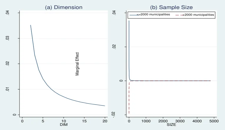
With regard the role of Dimension, we find that ˆ8 is positive: an increase in the number of inputs and/or outputs included in the frontier translates into an increase in the mean efficiency, so confirming the hypothesis of a positive link between the goodness of fit and the level of efficiency. Nguyen and Coelli (2009), Ogundari and Brümmer (2011) and Thiam et al. (2001) found a positive impact of Dimension on efficiency. Due to the use of logs, the marginal effect is 0.009 when Dimension is 8 (close to 8.15, which is the overall mean of
our sample; 8.35 is the average level of dimension for nonparametric studies) (ˆ8 0.0705 in model 3, ˆ80.0685 in model 6). Figure 6a highlights the pattern of the marginal effect on mean efficiency when Dimension ranges between its minimum and maximum values: when
the number of inputs and outputs equal to 7, the marginal effect of Dimension of efficiency
tends to 0.
The analysis of the relationship between bank efficiency and the number of observations used in estimating the frontier produces interesting findings. The continuous variable Sample Size enters our regressions in log form as we try to control for a potential
non-linear effect. It is likely that the impact of sample size diminishes as the observations increase. We also introduce the interaction term lSIZE*MANY to verify whether the effect of
sample size differs between an analysis conducted on a number of municipalities <2000 and an analysis conducted on a number of municipalities >2000. In model 3, the parameter
ˆ
10 isnegative (-0.055), thus when estimations refer to larger numbers of municipalities the effect of Sample Size becomes negative(figure 6b).
5.5 The role of country-observables
21
[image:22.595.111.487.354.572.2]efficiency study on local government. As far as corruption is concerned, we find that the coefficient of the CPI index is always significant and whatever the model we consider (it is 0.007 in models 5 of tables 2 and 3). As high levels of the CPI index are for countries with low corruption, the MRA results show that the efficiency studies for local government in countries with low corruption yields, on average, higher efficiency scores than the studies focusing on more corrupted countries. The main explanation is that low corruption is a crucial component of good local government and institutional quality because it discourages rent-seeking activities (del Sol, 2013). Similarly, regressions with the ILS index confirm the role of institutions; the coefficient of ILS index is 0.024 when considering all the samples (model 6 of table 2) and 0.031 when limiting the MRA to nonparametric studies (model 6 of table 3). It is proven that efficiency papers focusing on countries with high security of property rights and that are well protected by the rule of law, that is, with the foundations for economic freedom, yield, on average, higher efficiency scores than the studies focusing on countries with a weak legal system.13
Figure 6 Marginal effects of dimension and sample size
13
It is important to point out that the GDP per capita, the corruption, and the ILS index are highly correlated (data are available upon request). This explains why they enter into regressions one-by-one.
0
.0
1
.0
2
.0
3
.0
4
0 5 10 15 20
DIM
(a) Dimension
-.
02
0
.0
2
.0
4
Ma
rg
in
al
E
ffe
ct
0 1000 2000 3000 4000 5000
SIZE
<=2000 municipalities >2000 municipalities
22 Table 2 Meta-regression analysis of local governments efficiency scores (All sample)
Variables Model 1 Model 2 Model 3 Model 4 Model 5 Model 6
Constant 0.9284 *** 20.71 *** 18.87 *** 21.99 *** 18.16 ** 13.33 *
1/S -0.000011 ** -0.000006 0.000011 0.000008 -0.00001 0.0000007
DREG -0.1464 *** -0.1158 -0.1685 *** -0.2327 *** -0.2024 *** -0.2171 ***
EUROPE -0.1544 ** -0.0945 * -0.1748 *** -0.2288 *** -0.1494 *** -0.1852 ***
TE 0.0759 0.1799 ** 0.2034 *** 0.1236 0.3682 *
PANEL 0.1667 *** 0.1103 ** 0.0805 *** 0.1127 *** 0.0698 *
PARAM 0.1500 0.1646 * 0.1811 ** 0.1782 0.4081 *
Year of publication -0.0100 *** -0.0092 *** -0.0107 *** -0.0090 ** -0.0065 *
lDIM 0.0399 0.0705 * 0.0533 *** 0.1599 *** 0.0866 ***
lSIZE -0.0006 0.0355 ** 0.0240 *** 0.0110 0.0184 *
lSIZE*MANY -0.0548 *** -0.0472 *** -0.0328 *** -0.0599 ***
GDP per capita 0.0056 ***
CPI 0.0073 ***
ILS 0.0240 **
Observations 308 294 294 290 208 202
tau2 (between-study variance) 0.0192 0.0171 0.0121 0.0117 0.0072 0.0131
% residual variation due to
heterogeneity 99.94% 74.22% 70.16% 69.51% 70.67% 71.78%
Adj R-squared 31.63% 41.58% 58.60% 60.36% 77.54% 60.32%
F- Fisher 23.86 13.32 19.08 18.53 24.59 13.73
Legend: * p<0.2; ** p<0.1; *** p<0.05.
23 Table 3 Meta-regression analysis of local governments efficiency scores from nonparametric studies
Variables Model 1 Model 2 Model 3 Model 4 Model 5 Model 6
Constant 5.06 1.46 3.65 13.65 *** 13.90 * 20.55 **
1/S 0.000002 -0.000014 0.000003 -0.000003 -0.000010 0.000003
DREG -0.2466 *** -0.2032 ** -0.2527 *** -0.3757 *** -0.2120 *** -0.2645 ***
EUROPE -0.2340 *** -0.1608 *** -0.2369 *** -0.3500 *** -0.1749 *** -0.2311 ***
TE 0.2152 ** 0.0949 0.2003 * 0.2519 *** 0.1518 0.4926 **
PANEL 0.1099 ** 0.1802 *** 0.1217 *** 0.0673 *** 0.1206 *** 0.0621
FDH 0.2308 *** 0.2918 *** 0.2454 *** 0.2211 *** 0.1845 *** 0.1599 **
Year of publication -0.0022 -0.0003 -0.0015 -0.0065 ** -0.0069 * -0.0102 **
lDIM 0.0756 ** 0.0376 0.0685 ** 0.0401 * 0.1631 *** 0.1081 ***
lSIZE 0.0022 -0.0308 * 0.0050 -0.0136 0.0024 0.0040
lSIZE*MANY -0.0533 *** -0.0520 *** -0.0396 *** -0.0280 *** -0.0607 ***
VRS 0.0657 ** 0.0544 ** 0.0778 *** 0.0477 * 0.0441 *
GDP per capita 0.0104 ***
CPI 0.0073 ***
ILS 0.0309 ***
Observations 267 267 267 263 184 178
tau2 (between-study variance) 0.0097 0.0137 0.0091 0.0077 0.0070 0.0098
% residual variation due to heterogeneity 70.58% 70.55% 66.28% 64.22% 71.30% 71.58%
Adj R-squared 67.99% 54.64% 69.86% 75.70% 78.88% 71.04%
F- Fisher 25.16 17.74 24.24 26.77 23.27 16.47
Legend: * p<0.2; ** p<0.1; *** p<0.05.
24
6. Conclusions
This paper collected 360 observations of local government efficiency from 54 primary studies published from 1993 to 2016. It used a meta-analysis to evaluate the impacts of a number of related factors on the heterogeneity of efficiency in primary studies. Results show that methodological choices and some country-observables cause heterogeneity in results that one observes when referring to the worldwide literature of local government efficiency.
First of all, it is noteworthy to point out that the descriptive section of our meta-dataset highlights the fact that efficiency scores are highly heterogeneous. To be precise, significant differences in means are found when grouping efficiency on the basis of different criteria. For instance, cost efficiency is significantly lower than production efficiency. Furthermore, the unconditioned mean of efficiency scores from parametric studies is higher than that from nonparametric studies. Within the latter, the average of efficiency in DEA papers is lower than that collected from FDH studies. Besides differences in