Numerical Simulation of Foaming Processes

(1)

http://www.scirp.org/journal/wjm ISSN Online: 2160-0503

ISSN Print: 2160-049X

DOI: 10.4236/wjm.2017.711024 Nov. 29, 2017 297 World Journal of Mechanics

Numerical Simulation of Foaming Processes

Katharina Gladbach

1

, Antonio Delgado

1

, Cornelia Rauh

1,2

1_{Institute for Fluid Mechanics, Friedrich-Alexander-University Erlangen-Nuremberg,}_{Erlangen, Germany} 2_{Institute for Food Technology and Food Chemistry, Technical University Berlin, Berlin, Germany}

Abstract

The literature model studied in this article describes bubble formation and growth in a highly viscous polymer liquid with support of a gaseous matter dispersed under pressure before foaming. The foam growth is induced by the application of vacuum and mass transport of volatile components dissolved in the polymer liquid. Based on this literature model, aeration processes are cal-culated for intermediate viscosity and low viscosity biological systems, as they are of interest for biomatter foams, in particular for food foams in industrial processes. At the end of this article, the numerical results are presented and discussed.

Keywords

Foaming Process, Conservation Equations, Finite Difference Method, Convergence Analysis, Reynolds Number, Newtonian Liquids

1. Introduction

Foams are of essential importance in nature and in a wide range of technical fields that deal with matter of biological origin such as biotechnology as well as food production and beverage industry. There are several methods to incorpo-rate bubbles within the biomatter structures: mixing, steam generation, gas in-jection, vacuum expansion and fermentation to name the most important pro-cedures [1]. Recent experimental studies [2]-[7] have established relationships between process parameters and dispersion characteristics. However, there is still a lack of mathematically well-founded physical models that describe bubble formation and behavior in biomatter adequately.

Piesche, Nonnenmacher and Schütz [8][9][10] developed models to calculate foaming processes of polymer liquids in a static degassing system, which is sup-ported by a gas dispersed into the polymer liquid under pressure before foaming.

How to cite this paper: Gladbach, K., Delgado, A. and Rauh, C. (2017) Numerical Simulation of Foaming Processes. World Journal of Mechanics, 7, 297-322.

https://doi.org/10.4236/wjm.2017.711024

Received: November 1, 2017 Accepted: November 26, 2017 Published: November 29, 2017

http://creativecommons.org/licenses/by/4.0/

(2)

DOI: 10.4236/wjm.2017.711024 298 World Journal of Mechanics The foam growth is induced by a pressure drop and diffusion of volatile compo-nents dissolved in the polymer liquid. The related fluid mechanical transport processes are divided into two consecutive models that concern spherical foam and polyhedral foam, respectively. The foam growth is calculated by solving problem-specific conservation equations for mass, momentum and thermal energy. In the present article, the models proposed in [8][9][10] are adopted to calculate aeration processes of biomatter. Usually, aeration occurs by applying vacuum or including the gas phase into the liquid phase with a high pressure. Since material parameters for modeling diffusion processes inside biomatter foams do not exist in the literature, they are estimated to illustrate the influence of possible variations.

The model equations [9] are first specified, and the numerical procedures used for solving the model equations in Matlab [11] [12][13] [14] [15] are outlined. A convergence analysis [16] [17] confirms that the numerical me-thod converges with order 2 in space and at least with order 1 in time. In con-trast to the literature [8] [9][10], where foaming processes of highly viscous polymer melts are calculated and the Reynolds numbers are Re  1 so that inertia terms in the momentum equation can be neglected [8] (p. 63), foaming processes of food systems [1]-[7] with Reynolds numbers Re ≈ 1 are now calcu-lated. The Reynolds numbers Re ≥ 1 require that inertia terms in the momentum equation have to be taken into account since inertial forces and viscous forces are likewise relevant. At the end of this article, the numerical results are plotted, discussed and compared both with the results presented by Piesche, Nonnen-macher and Schütz [9][10] for polymer foams and the results given by Haedelt, Beckett and Niranjan [2][3] for aerated chocolate as a representative of matter of biological origin.

2. Model Equations for Foaming Processes

For the sake of completeness, it is stated that the following considerations post-ulate physically existent, stable and mathematically unique solutions of the non-linear transport equations for mass, momentum and thermal energy [8][9] [10]. As mentioned above, mimicking foaming processes occurs by employing two models that describe spherical foam and polyhedral foam, respectively. The model for the spherical foam is based on the assumption that, at the beginning of a foaming process, small monodisperse spherical bubbles are already present in the highly viscous liquid. The bubbles are arranged in a regular cubic spatial structure, see Figure 1 (left). Each elementary cell includes four bubbles, which are composed proportionately. The foam volume of an elementary cell at time t = 0 is given by

3 ,0 e

ges,0

V,0

16

V π

3 c

B

r

= _{, (1)}

(3)

[image:3.595.214.533.72.203.2]

DOI: 10.4236/wjm.2017.711024 299 World Journal of Mechanics

Figure 1. Spherical foam model (left) and growth of a single spherical bubble (right) [9].

g,0 g,0

V,0

ges,0 g,0 f

V V

c

V V V

= =

+ . (2)

The total foam volume Vges,0 at time t = 0 is composed of the gas volume Vg,0 of the bubbles and a liquid volume Vf. The liquid volume that surrounds the bubbles of an elementary cell is constant, regardless of the time:

e 3

f ,0

V,0

16 1

V π 1

3 rB c

  = _ − _

 . (3)

The first model is used to describe the initial phase of foaming until the bub-bles begin to influence each other and polyhedral bubbub-bles are formed. In the second model, the monodisperse spherical bubbles are substituted by monodis-perse pentagon dodecahedron bubbles. The surface OD and volume VD of a do-decahedron bubble are calculated from the edge length aD of the equilateral pen-tagon, i.e.

2 D

O =3 25 10 5+ ⋅a_D, (4)

(

)

3

D

1

V 15 7 5

4 aD

= + ⋅ . (5) The constant liquid volume e

f

V 4 is arranged in a thin layer normal to the

surface of the respective bubble. The next three subsections are dedicated to the model equations, which are adopted from the literature [8][9][10].

2.1. Model Equations for the Spherical Foam

(4)

cur-DOI: 10.4236/wjm.2017.711024 300 World Journal of Mechanics rent bubble radius rB(t):

1 3

3 3

,0

V,0

π 1

1 c 3 2

S B B

r =_r _ − +_ r _

 

  . (6)

Equation (6) determines the integration limits for the conservation equations. As shown in [9], the conservation equation for mass in the liquid phase simpli-fies to an expression for the radial velocity component (see also Figure 1, right)

( )

22

d d

,

d d

B B

r r

r u r t

t r t

= = ⋅ _{. (7)} Similarly, the simplified momentum equation in radial direction r for the sin-gle velocity component u is given by

(

)

2

rr rr

u u p

u

t r r r r θθ

τ

ρ

_∂ + ∂ _= −∂ +∂ +

τ

−

τ

∂ ∂ ∂ ∂

  , (8)

where p is the pressure, τrr and τθθ are the normal stresses in radial and polar di-rection, σ is the interface tension and ρ is the density of the liquid [9]. Inserting the continuity Equation (7) into the momentum Equation (8) and integrating the momentum equation within the limits r = rB(t) and r = rS(t) gives the non-linear, integro-differential equation of motion

(

)

2

2 4

2

2 4

d d

1 1 1

4 3

2 d

d

2 1

2 d

S

B

B B B B

B

B S S S

r

g rr

r B

r r r r

r

r r t r r t

p p r

r r θθ

ρ

σ _τ _τ

∞

  ₋  ₊  ₋ ₊        _ _ 

     

 

= − − +

∫

−

(9)

to be solved. Equation (9) assumes that due to the large density differences be-tween the liquid and gaseous phase, no tangential momentum exchange occurs between both phases. The ambient pressure and pressure inside a bubble are in-terlinked by

( )

S rr

( )

S

p_∞ t = p r −τ r , (10)

( )

2

g B rr B

B

p t p r r

r

σ τ

= − + _{. (11)}

The integral on the right side of Equation (9) characterizes the tensile stresses around the bubble. With regard to the rheological behavior of the liquid, New-tonian, i.e. purely viscous liquids are only considered here. The rheological equ-ation of state for an incompressible Newtonian liquid is S = 2η0D, where S is the extra stress tensor, D is the deformation velocity tensor and η0 is the zero-shear viscosity of the liquid. The normal stress difference in (9) reads then

2

0 0 3

d

2 6

d

B B

rr

r r

u u

r r r t

θθ

τ −τ = η _∂ − _= −η ⋅ ∂

  . (12)

(5)

DOI: 10.4236/wjm.2017.711024 301 World Journal of Mechanics mass transport of the volatile components from the liquid into a bubble is based on the assumptions that the ideal gas law is valid, the components do not influ-ence each other and the concentrations ξi of the components are low so that the Henry law can be applied [9]. Hence, the concentration equation for each com-ponent i reads

2 2

1

D

i i i

i

u r

t r r r r

ξ ξ ξ

∂ ₊ ∂ ₌ ∂  ∂   

∂ ∂ ∂  ∂ , (13)

where Di is the diffusion coefficient [9]. Due to the mass transport, a mass bal-ance equation for each component i in the gas phase has to be taken into ac-count [9]:

( )

3 2

d

3 D d

B

i

B i i B

r r

r r

t r

ξ

ρ

= ∂

= ⋅

∂ . (14) By assuming a homogeneous temperature field inside the bubble, characte-rized by ϑ(r = rB), the partial pressure pi in the gas phase is calculated by

(

)

R

i i i B

p =ρ ⋅ ⋅ϑ r=r , where R_i and ρ_i, respectively, are the specific gas constant and the density of the component i. The total pressure pg inside the bubble is the sum of all partial pressures. According to Henry’s law, the concentration of a gas dissolved in a liquid is proportional to the pressure of the respective gas in the gaseous phase. The equilibrium gas concentration and thus the first boundary condition to solve the concentration equation have to be formulated adequately, that is ξGL,i = pi/HW,i, where HW,i is the Henry coefficient of the component i. Due to the mass transport, a transport of thermal energy between the phases also takes place. Further simplified assumptions apply: (i) adiabatic foaming process, (ii) when considering a single bubble, pure one-dimensional heat conduction in radial direction, (iii) negligible production of internal energy by viscous dissipa-tion or diffusion. Under these premises, the transport of thermal energy is ex-pressed by

2 W 2

1

c u r

t r r r r

ϑ

ρ

_∂ + ∂ _= ∂ _

λ

∂ _

∂ ∂ ∂ ∂

   , (15)

where λW is the heat conductivity and c is the specific thermal capacity of the liquid [9]. Solving the temperature Equation (15) requires knowing the temper-ature gradient at the phase boundary as the first boundary condition, i.e.

(

2

)

W S, 2

1 d D h

d

B B

i

i i B

i

r r r r B

r

r r r t

ξ

ϑ

λ

ρ

σ

= =

∂ ∂

⋅ = ∆ ⋅ + ⋅

∂

∑

∂ , (16)

where ΔhS,i is the absorption enthalpy of the component i[9]. Equation (16) is completed by work, which is performed to enlarge the bubble surface.

(6)

DOI: 10.4236/wjm.2017.711024 302 World Journal of Mechanics (i) The gas volume and liquid volume remain unchanged. (ii) The time deriv-ative of the volume of a bubble is maintained. (iii) The partial pressures in the gaseous phase remain unchanged. (iv) The concentration and temperature pro-files are transformed with respect to the constant liquid volume. According to the first condition (i), the edge length aD,begin2 of a pentagon dodecahedron bub-ble at the beginning of the second model is calculated from the radius rB,end1 of a spherical bubble at the end of the first model:

(

)

1 3

,begin2 ,end1

16π 3 15 7 5

D B

a r

 

 

=_ _

+

 

. (17)

The liquid volume e f

V 4 is transformed into a thin layer normal to the

bub-ble surface with thickness

e f begin2

2 ,begin2

V 4

3 25 10 5 _D

h

a

=

+ ⋅ . (18)

The second condition (ii) for the model change leads to the time derivatives

d 1 d

d 2 d

D D

a a h

t = − ⋅ h ⋅ t , (19)

begin2 begin2 ,end1

,end1

d d

2

d d

B B

h h r

t = − ⋅r ⋅ t . (20)

2.2. Model Equations for the Polyhedral Foam

In the second model, the bubbles are assumed to have the idealized shape of a pentagon dodecahedron. The liquid volume is transformed into a thin layer normal to the surface of the bubbles. According to the model assumption, two neighboring bubbles share a liquid lamella, i.e. the calculations are limited to one half of the liquid lamella. The conservation equations for a liquid lamella are formulated in cylindrical coordinates (r, φ, z) with the velocities u in radial di-rection and w in axial direction. The geometrical formulation in cylindrical coordinates is based on the assumption that the stress state within a side surface of a pentagon dodecahedron bubble does not differ significantly from the stress state within a circular side surface of same area [9]. Figure 2 depicts schemati-cally a liquid layer with height h(t), which is surrounded by the Plateau edges, the gas phase of a dodecahedron bubble and the liquid layer of the neighboring dodecahedron bubble.

(7)

[image:7.595.225.525.76.174.2]

DOI: 10.4236/wjm.2017.711024 303 World Journal of Mechanics Figure 2. Pentagon dodecahedron bubble model [9].

( )

1 d

( )

,

2 d 2

r h r

u r t t

h t ε

= − ⋅ ⋅ = −  (21)

with the elongational rate

( )

, 1 d

( )

d

w z t h

t

z h t

ε

∂

= =

∂  . (22) The momentum equation in axial direction z simplifies to

zz

w w p

w

t z z z

τ

ρ

_∂ + ∂ _= −∂ +∂

∂ ∂ ∂ ∂

  . (23)

Inserting the relation (22) into the momentum Equation (23) and integrating the momentum equation within the limits z = 0 and z = h(t) gives the equation of motion to be solved. The balance of forces at the phase boundary to the bub-ble z = h(t) and at the Plateau edges of the liquid lamella z = 0 are taken into ac-count so that

( )

2 2

d

0 0

2 d g zz rr

h h

p p

t

ρ

= − + ∞−

τ

−

τ

 (24) in accordance to [9]. For a Newtonian liquid with zero-shear viscosity η0, the normal stress difference in (24) reads

0

3

zz rr

τ −τ = η ε. (25) The assumptions already made in the first model for the mass and energy transport also apply here in the second model [9]. After the transformation x= −h z, the concentration and mass balance equation for each component i are given by

d

D d

i i i

i

x

t t x x x

ξ ξ ξ

∂ ₊ _⋅∂ ₌ ∂  ∂   

∂ ∂ ∂  ∂ , (26)

(

D

)

D 0

d

V D O

d

i

i i

x

t x

ξ

ρ ρ

=

∂ = ⋅

∂ . (27)

The temperature equation and first boundary condition are given by

2 W

2

d

d c

x

t t x x

λ

ϑ ϑ ϑ

ρ

∂ ∂ ∂

+ ⋅ = ⋅

∂ ∂ ∂ , (28)

W S,

0 0

D h i

i i i

x x

ξ ϑ

λ ρ

= =

∂ ∂

⋅ = ∆ ⋅

(8)

2.3. Model Equations in the Dimensionless Form

The model Equations (9)-(16) for the spherical foam are subjected to the La-grange coordinate transformation

(

3 3

)

₃

B

y= r −r and transformed into di-mensionless equations [9]. Similarly, the model Equations (24)-(29) for the po-lyhedral foam are subjected to the Lagrange coordinate transformation 2

D

q=xa and transformed into dimensionless equations [9]. As shown in [9], the coordi-nate transformations ensure that the convective terms in the concentration and temperature Equations (13), (15), (26) and (28) are eliminated. From a dimen-sional analysis, a set of dimensionless π-numbers is obtained:

0.5 0

1 3

,0 ,0 ,0 ,0

,

B B

r p r p

η

σ

ρ

π

ρ

∞ ∞   = = _ _

  , (30)

0.5 0.5

,0 W

4, 5 6 0

,0 ,0 ,0 ,0 ,0

D

, , c

c

i i

B B

r p r p p

λ

ρ

π

ϑ

ρ

∞ ∞ ∞

   

= _ _ = _ _ =

    , (31)

7, 0 ,0 R i i p ρ π ϑ ∞

= _{. (32)}

The index 0 refers in each case to the time point t = 0, whereas the index i re-fers to a volatile component i dissolved in the liquid. The dimensionless quanti-ties are indicated by the corresponding capital letters.

The relevant quantities are the time

(

) (

)

0.5

,0 ,0

B

T= t r ⋅

ρ

∞

ρ

, the radius of a spherical bubble RB=

(

rB rB,0

)

, the outer radius of the liquid volume that surrounds a bubble RS=

(

r rS S,0

)

, the transformed spatial coordinate

(

3

)

,0

B

Y= y r , the normal stresses S_YY=

(

τ_yy ρ_∞_,0

)

and S_θθ =

(

τ_θθ ρ_∞_,0

)

, the temperature Θ =

(

ϑ ϑ0

)

, the pressure inside a bubble Pg=

(

pg p∞,0

)

and the ambient pressure P∞=

(

p∞ p∞,0

)

. The additional dimensionless quantities used for the polyhedral foam model are the thickness of a liquid lamella

(

B,0

)

H= h r , the edge length of a dodecahedron bubble A_D=

(

a_D r_B_,0

)

, the transformed spatial coordinate

(

3

)

,0

B

Q= q r and the corresponding normal stresses SZZ =

(

τ ρzz ∞,0

)

and SRR =

(

τ ρrr ∞,0

)

.

The model equations for the spherical and polyhedral foam in the dimension-less form with appropriate initial and boundary conditions [9][10] are now spe-cified.

Spherical foam:

Equation of motion at the phase boundary

2 2 4 2 2 4 1 3 0 d d

1 1 1

4 3 2 d d 2 2 d 3 S

B B B B

B

B S S S

Y YY g

B B

R R R R

R

R R T R R T

S S

P P Y

R Y R

θθ π ∞    ₋  ₊ ₋ ₊       _ _     − = − − + +

∫

(33)

(

0

)

1

B

R T = = and d

(

0

)

0 d

B

R T

T = = , where

(

)

3 3

1 3

S S B

(9)

DOI: 10.4236/wjm.2017.711024 305 World Journal of Mechanics 3 3 3 3 0 d 1

2 d 4 1

d 3

S

Y

YY B B

B

B S

S S R R

Y

R T

Y R R

θθ

π

 

− ₌ ₋

 

+ _ _

∫

(34)

Concentration equations

(

₃

)

4 3

4,

,0

D 3

D

i i i

i B

i

Y R

T Y Y

ξ _π  ξ 

∂ ∂ ∂

=  + 

∂ ∂ __ ∂ __ (35)

1 GL, 1 1

0, 0 : i i , i 0

T = Y = ξ₌ =ξ ₌ ξ_> = and T=0, 0< ≤Y YS:ξ ξi = i,0, GL,

0, 0 : _i _i

T> Y= ξ ξ= and 0, : i 0

S

T Y Y Y ξ

∂ > = =

∂ .

Mass balance equations

3 4 4, 0 ,0 D d 3 d D

i i i

B i B

Y i

R R

T Y

ρ _π ξ

ρ =

∂  

= ⋅

  _∂

  (36)

1,0 1 7,1 1 2 i ρ π ρ π

= ₌ + _and

1,0 0

i

ρ> = . Temperature equation

(

)

4 3

3

5 3Y RB

T

π

Y Y

∂Θ₌ ∂  ₊ ∂Θ

 

∂ ∂  ∂  (37)

S, 1

5 6 4, 3

0 ,0 ,0 0

h

D 2 d

D d

i

i i B

i i

Y i Y B

R

Y p Y R T

ρ ξ π

π π π

= ∞ =

∆ ∂ ∂Θ

⋅ = ⋅ +

∂

∑

∂ (38)

0, 0 S: 1

T= ≤ ≤Y Y Θ = ,

0, 0 :

T Y Y

∂Θ > =

∂ (Equation (38)) and T 0,Y YS: 0

Y

∂Θ > = =

∂ .

The pressure inside a bubble is determined by 7, 0

i

g i Y

i

P π ρ

ρ =

  =_ _⋅ Θ



∑

 .

Polyhedral foam:

Equation of motion at the phase boundary

(

)

2 2

d

2 d g ZZ RR

H H

P P S S

T = − + ∞− − (39)

(

*

)

begin2

H T =T =H and d

(

*

)

d begin2

d d

H H

T T

T = = T .

Newtonian liquid 3 1 d 3 d ZZ RR H S S H T π

− = ₍₄₀₎

Concentration equations 4 4, ,0 D D

i i i

i D i

A

T Q Q

ξ _π  ξ 

∂ ₌ ∂ ∂  

∂ ∂ __ ∂ __ (41)

* 2

,end1

, 0 D: i i

T=T ≤ ≤Q HA ξ ξ= ,

*

GL,

, 0 : i i

T>T Q= ξ ξ= and * 2

, : i 0

D

T T Q HA

Q

ξ ∂ > = =

(10)

3 4

4,

,0 0

D

d 25 10 5

12

d 15 7 5 D

i i i

D i D

i Q

A A

T Q

ρ

ξ

π

ρ

₌

∂

  +

= ⋅

  ₊ _∂

  (42)

Temperature equation 2 4

5AD 2

T π Q

∂Θ ∂ Θ =

∂ ∂ (43)

S,

5 6 4,

,0 ,0

0 0

h D

D

i

i i

i i i

Q Q

Q p Q

ρ

ξ

π π

π

∞

= =

∆ ∂ ∂Θ

⋅ = ⋅

∂

∑

∂ (44)

* 2

end1

, 0 _D:

T=T ≤ ≤Q HA Θ = Θ ,

*

, 0 :

T T Q

Q

∂Θ > =

∂ (Equation (44)) and

* 2

, D: 0

T T Q HA

Q

∂Θ > = =

∂ .

3. Numerical Method for Solving the Model Equations

The models developed in [9] [10] have been implemented with the software Matlab. The integro-differential Equations (33)-(38) and differential Equations (39)-(44) present two non-linear systems of equations that are treated consecu-tively. To solve the equations numerically, a finite difference discretization me-thod and a diagonally implicit Runge-Kutta meme-thod are applied. The discretized equations are solved separately from each other. The concentration and mass balance equations, the temperature equation and the equation of motion are solved in this order for each model. Since the equations are non-linear and coupled, they have to be solved iteratively in each time step. For the outer itera-tion process, a Picard iteraitera-tion method (fixed-point method with successive substitution) is used. In this section, discretization and solution of the inte-gro-differential Equations (33)-(38) in a time step for the first model are ex-plained. The same considerations apply to solving the differential Equations (39)-(44) for the second model numerically.

The concentration and temperature Equations (35) and (37) are parabolic partial differential equations. They are discretized using the finite difference method. As an example, the concentration Equation (35) for a gaseous compo-nent i is studied. The diffusion coefficient is assumed to be constant, that is Di = const. Applying the product rule gives the equation

(

)

(

)

2

1 3 4 3

3 3

4, 4 3 3 2

i i i

i Y RB Y RB

T Y Y

ξ

π



ξ



∂ ₌ ₊ ∂ ₊ ₊ ∂

 

∂ _ ∂ ∂ _. (45)

Equation (45) is discretized in Ω × Γ with Ω =

[

0,YS

]

and Γ =

[

0,Tend1

]

, where discretization is done first in space and then in time. Note that, in the fol-lowing, the indices n and k refer to discrete points in space and time. Note also that, in section 3 and section 4.1, the constant discretization parameter h denotes the spatial step size, not the thickness of a liquid lamella in the polyhedral foam. With the constant discretization parameter h=YS N, N∈, the set of all

spatial grid points is defined: Ω =_h:

{

Y_n∈Y_n= ⋅n hand 0≤ ≤n N

}

. The

(11)

DOI: 10.4236/wjm.2017.711024 307 World Journal of Mechanics equidistant.

The spatial derivatives in (45) are approximated by central difference quo-tients. Inserting the central difference quotients in (45) gives a coupled system of ordinary differential equations for the unknown functions of the gaseous com-ponents dissolved in the liquid, ξi

(

Y Tn,

)

, 1≤ ≤ −n N 1, that is

(

)

(

)

(

)

(

)

(

)

(

)

(

)

(

)

( )

1 3 ₁ ₁

3 4,

4 3 ₁ ₁

3 4, 2 2 4, , , , 3 4 2

, 2 , ,

3

i n i n i n

i n B

i n i n i n

i n B

i

Y T Y T Y T

Y R

T h

Y T Y T Y T

Y R

h O h

ξ ξ ξ

π

ξ ξ ξ

π π + − + − ∂ − = + ⋅ ⋅ ∂ − + + + ⋅ + ⋅ (46)

For the time discretization, the grid Γ =_k:

{

T_k∈T_k= ⋅k vand 0≤ ≤k K

}

is

selected, where the discretization parameter v=Tend1 K, K∈, is the

tem-poral step size. The system (46) is integrated by one-step-θ methods [16] [17]. The parameter θ∈

[ ]

0,1 determines the concrete difference scheme. If the right

side of Equation (46) is referred to as F Y Ti

(

n,

)

, the integration within the

lim-its T=Tk and T=Tk+1 gives

(

)

(

)

1 _, 1

d , d

k k k k T T i n i n T T Y T

T F Y T T

T

ξ

+ ∂ + = ∂

∫

(

)

(

)

(

) (

)

(

)

( )

1 1 2 4,

, , 1 , ,

i n k i n k i n k i n k

i

Y T Y T v F Y T F Y T

O v

ξ ξ θ θ

π

+  + 

⇔ − = ⋅_ − ⋅ + ⋅ _

+ ⋅ (47)

For θ∈

[ ]

0,1 , the Equations (47) have always accuracy order 2, since R_B(T_{k + 1})

is not known yet and RB(Tk) or an approximated value obtained after an itera-tion step has to be inserted. The following abbreviaitera-tions are now defined:

( )

(

₃

)

1 3

, : 4, 3 2

k

i n i n B k

F =π Y +R T ⋅ h, (48)

( )

(

)

4 3

3

, : 4, 3

k

i n i n B k

E =π Y +R T , (49)

2

: v

h

γ = _{. (50)}

Inserting the expressions for F Y Ti

(

n, k

)

and F Y Ti

(

n, k+1

)

in (47) gives the discretized equations for the variables ξ_i

(

Y T_n, _k

)

,1≤ ≤ −n N 1, that is

(

)

(

)

(

)

(

)

(

)

(

)

(

)

(

)

(

) (

)

(

)

(

)

(

)

(

)

(

)

(

)

, 1 , , 1 1

, , 1 1

, , , 1

2 2

, , 1 4,

1 2 , ,

,

1 2 1 , 1 ,

1 ,

k k k

i n i n k i n i n i n k

k k

i n i n i n k

k k k

i n i n k i n i n i n k

k k

i n i n i n k i

E Y T F E Y T

F E Y T

E Y T F E Y T

F E Y T O vh v

θγ ξ θγ ξ

θγ ξ

θ γ ξ θ γ ξ

θ γ ξ π

+ − + + + − + + ⋅ − − + ⋅ − + ⋅ = − − ⋅ + − − + ⋅ + − + ⋅ + ⋅ + (51)

For each discrete time point Tk, the grid function , :

k i h h

(12)

(

)

( )

(

)

( )

(

)

( )

(

)

(

)

( ) (

)

(

)

( )

(

)

(

)

( )

1 1

, , , , , 1

1

, , , 1

, , , , , 1

, , , 1

1 2

1 2 1 1

1

k k k k k

i n i h n i n i n i h n

k k k

i n i n i h n

k k k k k

i n i h n i n i n i h n

k k k

i n i n i h n

E Y F E Y

F E Y

E Y F E Y

F E Y

θγ ξ θγ ξ

θγ ξ

θ γ ξ θ γ ξ

θ γ ξ

+ + − + + − + + ⋅ − − + ⋅ − + ⋅ = − − ⋅ + − − + ⋅ + − + ⋅ (52)

Hence, the discrete solution is determined by a linear system of equations

1

, , , , ,

k k k k k

i h i h i h i h i h + ₌ ₊

L ξ M ξ b , (53)

(N 1) (N 1) N 1

, , , , , , ,

k k k k

i h i h i h i h

− × − −

∈_ ∈_

L M b ξ ,

that has to be solved in each time step. The initial and boundary conditions are taken into account by the vector ,

k i h

b , the first and the last component of which

are only non-zero. The matrix ,

k i h

L is diagonal if θ = 0 and tridiagonal

other-wise. The following one-step-θ methods are often used in practice: explicit Euler method of order 1 (θ = 0), implicit Euler method of order 1 (θ = 1) and, finally, Crank-Nicolson method of order 2 (θ = 0.5) [16][17]. If Ih is the identity matrix associated with the discretization, the matrix ,

k i h

L (similarly ,

k i h

M ) has the

form:

,

,1 ,1 ,1

,2 ,2 ,2 ,2 ,2

, N 2 , N 2 , N 2 , N 2 , N 2

, N 1 , N 1 , N 1

2 0 0

2 0

0 2

0 0 2

k i h h

k k k

i i i

k k k k k

i i i i i

k k k k k

i i i i i

k k k

i i i

E F E

F E E F E

F E E

θγ − − − − − − − − =  − −   ₋ ₋ ₋      + ⋅   − − −    ₋             L I (54)

The numerical analysis is based on the properties of M-matrices. In the ap-pendix, relevant definitions and theorems relating to M-matrices [14][15][16] [17] are summarized. Since θ∈

[ ]

0,1 ,

γ

>0 and 0 , ,

k k

i n i n

F E

< < _{is satisfied for} all spatial and temporal grid points if 0< <h 0.5 in (48)-(50), following prop-erties can be shown:

1) The matrix ,

k i h

L satisfies the sign condition in definition 1.

2) The matrix ,

k i h

L is diagonally dominant and irreducible.

According to theorem 1, ,

k i h

L is regular, according to theorem 2, ,

k i h

L is

even an M-matrix. Hence, the linear system of Equations (53) is uniquely solva-ble. For a vector w=1, it can be shown that ,

k i h ≥

L w 1, i.e.

(

,

)

1 2 ,

(

, ,

)

(

, ,

)

1

k k k k k k

i h _n= + θγEi n−θγ −Fi n+Ei n −θγ Fi n+Ei n =

L w for 2≤ ≤ −n N 2,

(

,

)

₁ 1 ,1 ,1 1

k k k

i h = +θγEi −θγFi ≥

L w for n=1,

(

,

)

_{N 1} 1 ,N 1 ,N 1 1

k k k

i h ₋ = +θγEi − +θγFi − ≥

L w for n= −N 1.

Hence, theorem 3 is applicable, and the following estimation is valid:

( )

1

, 1

k i h

−

∞≤

(13)

DOI: 10.4236/wjm.2017.711024 309 World Journal of Mechanics Estimation (55) is relevant for the convergence considerations in the next sec-tion. The Equation (46), 1≤ ≤ −n N 1 which is discretized in space, represents a

stiff system of ordinary differential equations. The greatest eigenvalue compared to the smallest eigenvalue behaves like O(h−2_{). Therefore, A-stable numerical} time integration procedures are required [16][17].

The temperature Equation (37) is discretized and solved similarly to the con-centration Equation (35). The mass balance Equation (36) is integrated by the one-step-θ method, which is also used for the concentration Equation (35). The equation of motion (33) is transformed into a system of first order inte-gro-differential equations. Since stiffness occurs, this system is solved by the TR-BDF2 method implemented in Matlab. The TR-BDF2 method is a diagonally implicit Runge-Kutta method of order 2 with associated error estimate of order 3 and is L-stable and also strongly S-stable [11][12][13]. For an incompressible Newtonian liquid, the integral in (33) can be calculated analytically so that the system depends only on time (see Equation (34)). The equation of motion (33) requires particularly a high computing time if a low-viscosity Newtonian liquid is given so that a small temporal step size has to be chosen.

4. Presentation and Discussion of Results

4.1. Considerations on Convergence

This section aims at proven convergence of the finite difference discretization method and its order [11]-[17]. The convergence considerations concern the transport processes of mass and thermal energy from the liquid in the gas phase. The convergence theory is based on the properties of the class of M-matrices and follows the numerical studies [16][17]. It is stated that the outer iteration me-thod gives convergent approximated values. The error function at time Tk is de-fined by

( )

, , ,

k k

i h= h iξ ⋅Tk − i h

e R ξ . (56)

Rh denotes the restriction operator that gives the exact solution of (45) in the spatial grid points at time Tk, whereas ,

k i h

ξ is the approximated solution. From (51)-(52), it follows that the finite difference method is consistent. The maxi-mum norm of the local truncation error ,

k i h

η is

(

2 2

)

, 4,

k

i h _∞=π i⋅O vh +v

η . (57)

Now, the global discretization error is studied. Note that, from (51)-(52), it follows

(

)

( )

, , 1 , , , ,

k k k k

i h h iξ ⋅Tk+ − i h h iξ ⋅Tk − i h= i h

L R M R b η . (58)

Applying ,

k i h

L to 1 ,

k i h

+

e gives

(

)

( )

1 1

, , , 1 , ,

, , , , , ,

, , ,

, ,

k k k k k

i h i h i h h i k i h i h

k k k k k k

i h h i k i h i h i h i h i h

k k k

i h i h i h

T

ξ ξ

+ +

+

= ⋅ −

= ⋅ + + − −

= +

L e L R L ξ

M R b η M ξ b

M e η

(14)

DOI: 10.4236/wjm.2017.711024 310 World Journal of Mechanics Hence, a recursion formula for the error function is obtained. Multiplying Equation (59) from left by the inverse matrix

( )

1

,

k i h

−

L and applying the maxi-mum norm gives

( )

1

( )

1

, , , , , ,

k k k k k k

i h i h i h i h i h i h

− −

+

∞ ≤ _∞ ∞ ∞+ _∞ ∞

e L M e L η . (60)

By recursive application, the following in equation is obtained:

( )

1 ₁ 0 , , , , 0 1 1 1 ₁ , , , 0 1 k

k l l

i h i h i h i h

l

k k

k

j j l

i h i h i h

l j l j l

− ₋ ∞ ₌ _∞ ∞ ∞ − − − ₋ ∞ ∞ ∞ = = = +   ≤       +    

∏

∑ ∏

∏

e L M e

L M η

(61)

The matrix norm of ,

k i h

M can be determined:

(

)

{

(

)

(

)

(

)

(

)

(

)

(

)

(

)

(

)

(

)

(

)

}

(

)

(

)

{

}

, , , ,

, , ,1 ,1 ,1

, N 1 , N 1 , N 1

, ,

max 1 2 1 1

1 , 1 2 1 1 ,

1 2 1 1

max 1 2 1 2 1 1,

k k k k

i h n i n i n i n

k k k k k

i n i n i i i

k k k

i i i

k k

n i n i n

E F E

F E E F E

E F E

E E

θ γ θ γ

θ γ θ γ θ γ

θ γ θ γ

∞ − − − = − − + − − + + − + − − + − + − − + − − + = − − + − = M (62)

hence , 1

k i h _∞=

M if

(

)

(

)

(

)

2 2 , , 2 , ₂ , , 1

2 1 1 , 0.5

2 1

2 , 0

k k

i n k i n

i n _k

i n

v h

E v h E

h E h E θ θ θ θ θ ∞ =  − ≤ ⇔ ≤ =_ = − _ =  (63)

Using (55) and (62) in (61), it follows

( )

(

)

1 ₁ 0 , , , , 0 1 1 1 1 ₁ , , , 0 1 1 0 , , 0 2 , 4, max

due to .

k

k l l

i h i h i h i h

l

k k

k

j j l

i h i h i h

l j l j l

l

i h l i h

k

i h i

k

T

O h v k

v π − ₋ ∞ ₌ _∞ ∞ ∞ ≤ − − − ₋ ∞ ∞ ∞ = = = + ≤ ∞ ∞ ∞ ≤ ⋅ + ⋅ ≤ + ⋅ = + ⋅ + =

∏

∑∏

∏

 

e L M e

L M η

e η

e

(64)

The finite difference method is consistent and stable and thus convergent. The stability results from the fact that ,

k i h

L are M-matrices and

( )

k_{i h}_, −1 1

(15)

4.2. Results of the Numerical Simulations

As a reference example, the foaming process of a two-phase system consisting of polystyrene, styrene and nitrogen is considered. The nitrogen was dispersed into polystyrene under pressure and is in form of small spherical bubbles, but also in dissolved form in polystyrene, whereas styrene is already dissolved in polysty-rene. The necessary material and process data are taken from the literature [9] [10], see Table 1 and Table 2. The time process of the pressure drop is given by

( )

(Kexp) ,max

t

p t

P e

p

− ∞ ∞

∞

= = , (65)

[image:15.595.207.540.341.515.2]

where Kexp = 0.6 s−1 is the pressure drop coefficient. The coefficient Kexp is chosen so that the minimal pressure p∞,min = 0.025 bar is reached from the maximal pressure p∞,max = 10 bar after about 10 seconds. The heat conductivity and spe-cific thermal capacity of polystyrene are specified by λW = 0.17 W/(m·K) and c = 1500 J/(kg·K). Note that, at time T = 0, the bubbles consist only of nitrogen. For T > 0, the gaseous components dissolved in polystyrene diffuse into the bubbles.

Table 1. Material data for the system polystyrene/styrene/nitrogen at 240˚C [9].

Material quantity Comment Value Unity

density ρ PS 950 kg/m3

zero-shear viscosity η0 5838 Pas

surface tension σ 0.03 N/m

diffusion coefficient D1 PS/N2 1.0 × 10−9 m2/s

diffusion coefficient D2 PS/styrene 3.4 × 10−10 m2/s

Henry coefficient HW,1 PS/N2 14000 bar

Henry coefficient HW,2 PS/styrene 30 bar

gas constant R1 N2 296.8 J/(kg·K)

gas constant R2 styrene 79.83 J/(kg·K)

Table 2. Process data for the system polystyrene/styrene/nitrogen at 240˚C [9].

Process quantity Comment Value Unity temperature ϑ constant 240 ˚C gas volume fraction cV,0 0.01 m3/m3

gas volume fraction cV,t* model change 0.7 m3/m3

bubble radius rB,0 100 μm

initial concentration ξ1,0 N2 0.072 %

initial concentration ξ2,0 styrene 0.1 %

pressure p∞,max = p∞,0 10 bar

pressure p∞,min 0.025 bar

[image:15.595.209.540.546.724.2]

(16)

DOI: 10.4236/wjm.2017.711024 312 World Journal of Mechanics In summary, foam growth is induced by dispersion of nitrogen, vacuum applica-tion and diffusion of the volatile components dissolved in polystyrene.

The dimensionless foam volume V is determined on the basis of an elementa-ry cell in the first model (see Equations (1)-(3)), i.e.

(

)

(

)

3 3 1

e ,0 V,0 ges 3 V,0 e 3 ges,0 ,0 V,0

16_π 16_π

c 1

V ₃ ₃

V 1 c 1

V _{16 π}

3 c B B B B r r R r − + −

= = = + − _{, (66)}

and on the basis of a single bubble and the constant liquid volume around it in the second model (see Equation (5)), i.e.

(

)

3

V,0

3

V 1 c 15 7 5 1

16π AD

 

= + _ + ⋅ − _

 . (67) The local considerations suggest the definition of a local Reynolds number that characterizes the foaming process. The Reynolds number is defined by

( )

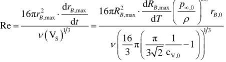
Re=q ν⋅l , where q is the volume flow rate, ν η ρ= is the kinematic vis-cosity and l is the length of the relevant flow region [18]. Selecting the volume flow rate, when the model changes from spherical to polyhedral foam, gives the local Reynolds number

( )

0.5 ,max ,0 2 ,max 2 ,max ,0 ,max

1 3 1 3

S

V,0

d

d ₁₆_π

16π

d d

Re

V ₁₆ _π ₁

π 1

3 3 2c

B B

B

R p

r _R _r

r T t ρ ν ν ∞   ⋅ _ _ ⋅   = =    −  _ _  _ _  

. (68)

The volume flow rate q is determined by the time derivative of the foam vo-lume e

ges

V in Equation (66). The maximal bubble radius can be calculated

ana-lytically, 1 3 1 V,0 ,max 1 V, * c 1 c 1 B t R − −  −  = _ _ −

  , (69) and is RB,max = 6.1358 in the examples studied here, whereas the time derivative dRB,max/dT has to be determined by simulation. The constant liquid volume VS surrounds the bubbles of an elementary cell in the first model:

(

3 3

)

3

S ,0

V,0

16 16 π 1

V π π 1

3 rS rB 3 rB 3 2c

 

= − = _ − _

 . (70)

If only spherical foam is formed, the volume flow rate q with the maximal time derivative dRB/dT is chosen. In this case, both quantities, the bubble radius

[image:16.595.248.474.362.424.2]

RB and its derivative dRB/dT, have to be determined by simulation.

(17)

[image:17.595.237.514.70.292.2]

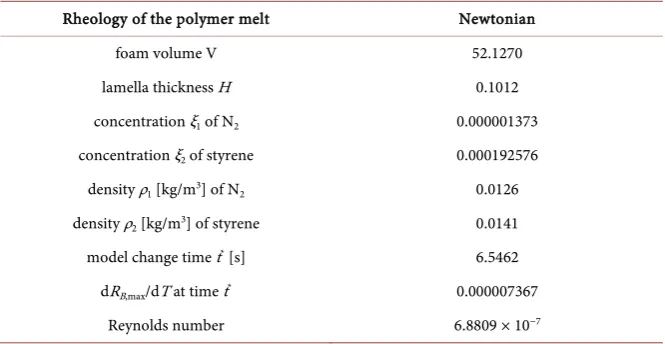
DOI: 10.4236/wjm.2017.711024 313 World Journal of Mechanics Figure 3. Bubble radius RB (red) in the first model, lamella thickness H

(green) in the second model and foam volume V (blue) as functions of the time T for the two-phase system polystyrene/styrene/nitrogen.

to Equation (65) and is constant after having reached the minimum. In Figure 3, the bubble radius RB (red), the lamella thickness H (green) and the foam volume V (blue) are plotted as functions of the time T over a period of 60 seconds. As expected, the bubble radius in the first model increases, the lamella thickness in the second model decreases and the foam volume increases continuously until a maximum value is reached. The model change from spherical foam to polyhe-dral foam is indicated by a point of discontinuity (black dotted line parallel to the y-axis) in the red/green graph. After 60 seconds, the foam volume has reached the maximum value.

(18)

[image:18.595.64.538.74.262.2]

DOI: 10.4236/wjm.2017.711024 314 World Journal of Mechanics Figure 4. Concentration profiles for nitrogen (left) and styrene (right) as functions of the normalized liquid volume around a bubble for the system polystyrene/styrene/nitrogen.

Table 3. Two-phase system polystyrene/styrene/nitrogen in equilibrium after foaming.

Rheology of the polymer melt Newtonian

foam volume V 52.1270

lamella thickness H 0.1012 concentration ξ1 of N2 0.000001373

concentration ξ2 of styrene 0.000192576

density ρ1 [kg/m3] of N2 0.0126

density ρ2 [kg/m3] of styrene 0.0141

model change time t*_[s] _6.5462

dRB,max/dT at time t* 0.000007367

Reynolds number 6.8809 × 10−7

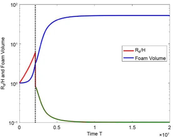
[image:18.595.207.540.326.498.2]

(19)

[image:19.595.216.535.62.322.2]

DOI: 10.4236/wjm.2017.711024 315 World Journal of Mechanics Figure 5. Bubble radius RB (red) in the first model, lamella thickness H (green) in the

second model and foam volume V (blue) as functions of the time T for different

two-phase systems without mass and heat transport during foaming.

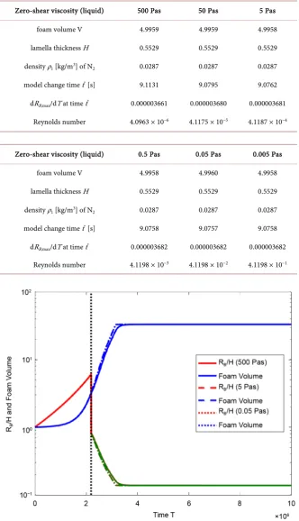
simulation results are plotted for the systems with the viscosity 500 Pas, 5 Pas and 0.05 Pas. It becomes apparent that the two-phase systems behave similarly during foaming and that they attain the same equilibrium state after foaming. The hydrodynamic equilibrium is reached after 10 or 20 seconds. Table 4 speci-fies the values of relevant material and process quantities after foaming and shows that the less viscous the liquid is, the faster the change from spherical to polyhedral foam occurs.

(20)

[image:20.595.208.541.101.680.2]

DOI: 10.4236/wjm.2017.711024 316 World Journal of Mechanics Table 4. Two-phase systems in equilibrium after foaming (without mass and heat transport).

Zero-shear viscosity (liquid) 500 Pas 50 Pas 5 Pas

foam volume V 4.9959 4.9959 4.9958

lamella thickness H 0.5529 0.5529 0.5529

density ρ1 [kg/m3] of N2 0.0287 0.0287 0.0287

model change time t*_[s] _9.1131 _9.0795 _9.0762

dRB,max/dT at time t* 0.000003661 0.000003680 0.000003681

Reynolds number 4.0963 × 10−6 _{4.1175 × 10}−5 _{4.1187 × 10}−4

Zero-shear viscosity (liquid) 0.5 Pas 0.05 Pas 0.005 Pas

foam volume V 4.9958 4.9960 4.9958

lamella thickness H 0.5529 0.5529 0.5529

density ρ1 [kg/m3] of N2 0.0287 0.0287 0.0287

[image:20.595.205.541.101.687.2]

Reynolds number 4.1198 × 10−3 _{4.1198 × 10}−2 _{4.1198 × 10}−1

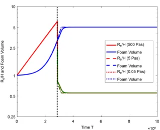
Figure 6. Bubble radius RB (red) in the first model, lamella thickness H (green) in the

second model and foam volume V (blue) as functions of the time T for different

(21)

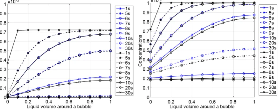
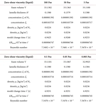
DOI: 10.4236/wjm.2017.711024 317 World Journal of Mechanics described above can also be made here: The two-phase systems, which differ on-ly in the viscosity of the liquid, behave similaron-ly during foaming and attain the same equilibrium state after foaming. Due to the mass and heat transport, a higher foam volume is reached than in the two-phase systems without diffusion. The concentration profiles of nitrogen and the flavoring substance in Figure 7 confirm that the flavoring substance desorbs faster in a low-viscosity liquid. To clarify the numerical simulation results, Table 5 contains the values of relevant material and process quantities after foaming. The hydrodynamic and thermo-dynamic equilibrium between the liquid and gas phase is reached after 20 seconds, i.e. pressure differences between the bubbles and their environment and concentration differences in the liquid are balanced.

Table 3 shows that another equilibrium state for the polymer system is reached, which can be explained by the higher temperature 240˚C, compared to the lower temperature 20˚C of the systems characterized in Table 5 after foam-ing. A local Reynolds number Re ≈ 1 is obtained in each case. Generally, the de-finition of a global Reynolds number would give values Re ≳ 1 in the Table 4, Table 5.

[image:21.595.69.539.509.694.2]

At the end, the simulation results are compared with the experimental results presented by Haedelt, Beckett and Niranjan [2] [3]. The authors investigated bubble formation in liquid tempered chocolate, which is an example of an in-termediate viscosity food system. After the tempering procedure, nitrogen (or another gas) was injected into the chocolate mass under controlled pressure and finely dispersed using a stator and rotor arrangement. When the mixture was returned to atmospheric pressure, the gases dissolved in the chocolate desorbed, and bubbles were formed [2][3]. The operating conditions were chosen as fol-lows: system pressure p∞,max = 4.5 bar, p∞,min = 1.0 bar, chocolate temperature ϑ0 = 30˚C [3] (p. E139). The remaining data not determined are taken from the Table 1, Table 2, but now pressure drop coefficient Kexp = 0.15 s−1, bubble radius

(22)

[image:22.595.210.539.90.441.2]

DOI: 10.4236/wjm.2017.711024 318 World Journal of Mechanics Table 5. Two-phase systems in equilibrium after foaming (with mass and heat transport).

Zero-shear viscosity (liquid) 500 Pas 50 Pas 5 Pas foam volume V 33.1302 33.1363 33.1100 lamella thickness H 0.1380 0.1379 0.1380 concentration ξ1 of N2 0.000001392 0.000001392 0.000001392

concentration ξ2 0.000183755 0.000183739 0.000183717

density ρ1 [kg/m3] of N2 0.0224 0.0224 0.0224

density ρ2 [kg/m3] 0.0236 0.0236 0.0236

Reynolds number 7.5492 × 10−6 _{7.5481 × 10}−5 _{7.5470 × 10}−4

Zero-shear viscosity (liquid) 0.5 Pas 0.05 Pas 0.005 Pas foam volume V 33.1101 33.1067 32.9925 lamella thickness H 0.1380 0.1380 0.1384 concentration ξ1 of N2 0.000001392 0.000001392 0.000001392

concentration ξ2 0.000183716 0.000183714 0.000183714

density ρ1 [kg/m3] of N2 0.0224 0.0224 0.0224

density ρ2 [kg/m3] 0.0236 0.0236 0.0236

Reynolds number 7.5470 × 10−3 _{7.5470 × 10}−2 _{7.5470 × 10}−1

rB,0 = 25 μm and chocolate viscosity η0 = 10 Pas. Furthermore, ρ = 1000 kg/m3 and σ = 0.072 N/m.

The simulations results plotted in Figure 8 over a period of 30 seconds show that a fine spherical foam is obtained. The maximal bubble radius is rB,max = 0.0882 mm, and the gas volume fraction is cV,t = 0.3073 in agreement with the experimental results [3] (p. E141) for aerated chocolate produced by using ni-trogen. The low gas volume fraction cV,t is especially a result of the moderate pressures p∞,max and p∞,min chosen, see also Table 6.

(23)

[image:23.595.221.529.63.313.2]

DOI: 10.4236/wjm.2017.711024 319 World Journal of Mechanics Figure 8. Bubble radius RB (red) and foam volume V (blue) as functions of the time T for

liqiuid tempered chocolate with dissolved gases.

Table 6. Two-phase system chocolate/flavor additive/nitrogen in equilibrium after foaming.

Rheology of the chocolate mass Newtonian

foam volume V 1.4293

maximal bubble radius RB,max 3.5284

concentration ξ1 of N2 0.000070609

concentration ξ2 0.000926433

density ρ1 [kg/m3] of N2 1.0993

density ρ2 [kg/m3] 0.1149

maximal time derivative dRB/dT 0.000000345

Reynolds number 3.8303 × 10−7

5. Conclusions

[image:23.595.227.539.390.543.2]

(24)

DOI: 10.4236/wjm.2017.711024 320 World Journal of Mechanics faster the hydrodynamic and thermodynamic equilibrium is reached, i.e. pres-sure differences between the bubbles and their environment and concentration differences in the liquid are balanced. The numerical method used for solving the model equations was analyzed with respect to stability, consistency and con-vergence in order to ensure accurate numerical simulation results, which are of interest e.g. for food foams in industrial processes.

Acknowledgements

This research project was supported by the German Ministry of Economics and Technology and the FEI (Forschungskreis der Ernährungsindustrie e.V., Bonn). Project AiF 17125 N. This project is part of the cluster “Proteinschäume in der Lebensmittelproduktion: Mechanismenaufklärung, Modellierung und Simula-tion” funded by the FEI and the AiF.

References

[1] Campbell, G.M. and Mougeot, E. (1999) Creation and Characterisation of Aerated

Food Products. Trends in Food Science & Technology, 10, 283-296.

https://doi.org/10.1016/S0924-2244(00)00008-X

[2] Haedelt, J., Pyle, D.L., Beckett, S.T. and Niranjan, K. (2005) Vacuum-Induced

Bub-ble Formation in Liquid-Tempered Chocolate. Journal of Food Science, 70,

E159-E164.https://doi.org/10.1111/j.1365-2621.2005.tb07090.x

[3] Haedelt, J., Beckett, S.T. and Niranjan, K. (2007) Bubble-Included Chocolate:

Re-lating Structure with Sensory Response. Journal of Food Science, 72, E138-E142.

https://doi.org/10.1111/j.1750-3841.2007.00313.x

[4] Jimenez-Junca, C., Sher, A., Gumy, J.-C. and Niranjan, K. (2015) Production of Milk Foams by Steam Injection: The Effects of Steam Pressure and Nozzle Design.

Journal of Food Engineering, 166, 247-254.

https://doi.org/10.1016/j.jfoodeng.2015.05.035

[5] Huppertz, T. (2010) Foaming Properties of Milk. A Review of the Influence of

Composition and Processing. International Journal of Dairy Technology, 63,

477-488.https://doi.org/10.1111/j.1471-0307.2010.00629.x

[6] Kamath, S., Huppertz, T., Houlihan, A.V. and Deeth, H.C. (2008) The Influence of

Temperature on the Foaming of Milk. International Dairy Journal, 18, 994-1002.

https://doi.org/10.1016/j.idairyj.2008.05.001

[7] Dickinson, E. (1997) Properties of Emulsions Stabilized with Milk Proteins.

Over-view of Some Recent Developments. Journal of Dairy Science, 80, 2607-2619.

https://doi.org/10.3168/jds.S0022-0302(97)76218-0

[8] Nonnenmacher, S. (2003) Numerische und experimentelle Untersuchungen zur

Restentgasung in statischen Entgasungsapparaten. Dissertation, VDI Verlag Düsseldorf.

[9] Piesche, M., Nonnenmacher, S. and Schütz, S. (2008) Modelluntersuchungen zur Restentgasung von Kunststoffschmelzen mit gasförmigen Schleppmitteln in einem statischen Entgasungsapparat. 1. Teil: Modellierung des Wachstums eines geschlossenzelligen Polymerschaums. Chemie Ingenieur Technik, 80, 659-675.

https://doi.org/10.1002/cite.200700179

(25)

Restentgasung von Kunststoffschmelzen mit gasförmigen Schleppmitteln in einem statischen Entgasungsapparat. 2. Teil: Durchführung und Ergebnisse der Schäumversuche. Chemie Ingenieur Technik, 80, 945-956.

https://doi.org/10.1002/cite.200700180

[11] Alexander, R. (1977) Diagonally Implicit Runge-Kutta Methods for Stiff O.D.E.’s.

SIAM Journal on Numerical Analysis, 14, 1006-1021.

https://doi.org/10.1137/0714068

[12] Hosea, M.E. and Shampine, L.F. (1996) Analysis and Implementation of TR-BDF2.

Applied Numerical Mathematics, 20, 21-37.

https://doi.org/10.1016/0168-9274(95)00115-8

[13] Prothero, A. and Robinson, A. (1974) On the Stability and Accuracy of One-Step

Methods for Solving Stiff Systems of Ordinary Differential Equations. Mathematics of Computation, 28, 145-162.https://doi.org/10.1090/S0025-5718-1974-0331793-2

[14] Deuflhard, P. and Bornemann, F. (2008) Numerische Mathematik 2. Walter de

Gruyter, Berlin, New York.

[15] Stoer, J. and Bulirsch, R. (2000) Numerische Mathematik 2. Springer-Verlag, Berlin,

Heidelberg, New York.https://doi.org/10.1007/978-3-662-09025-1

[16] Bärwolff, G. (2012) Numerik partieller Differentialgleichungen. Skript. Technische Universität Berlin, Fakultät II: Mathematik und Naturwissenschaften.

[17] Bastian, P. (2008) Numerische Lösung partieller Differentialgleichungen. Skript. Universität Stuttgart, Fakultät 5: Informatik, Elektrotechnik und Informationstechnik.

[18] Spurk, J.H. (1992) Dimensionsanalyse in der Strömungsmechanik. Springer-Verlag,

Berlin, Heidelberg, New York.

[19] Oldroyd, J.G. (1953) The Elastic and Viscous Properties of Emulsions and

Suspen-sions. Proceedings of the Royal Society of London A, 218, 122-132.

https://doi.org/10.1098/rspa.1953.0092

[20] Oldroyd, J.G. (1958) Non-Newtonian Effects in Steady Motion of Some Idealized

Elastico-Viscous Liquids. Proceedings of the Royal Society of London A, 245,

278-297.https://doi.org/10.1098/rspa.1958.0083

[21] Böhme, G. (2000) Strömungsmechanik nichtnewtonscher Fluide. Leitfäden der

angewandten Mathematik und Mechanik. B. G. Teubner: Stuttgart, Leipzig, Wiesbaden.https://doi.org/10.1007/978-3-322-80140-1

[22] Giesekus, H. (1994) Phänomenologische Rheologie. Eine Einführung. Springer-

Verlag, Berlin, Heidelberg, New York.https://doi.org/10.1007/978-3-642-57953-0

[23] Gladbach, K., Delgado, A. and Rauh, C. (2014) Modelling and Simulation of the

Transport of Protein Foams. Proceedings in Applied Mathematics and Mechanics,

14, 859-860.https://doi.org/10.1002/pamm.201410410

[24] Gladbach, K., Delgado, A. and Rauh, C. (2016) Modelling and Simulation of Food

Foams. Proceedings in Applied Mathematics and Mechanics, 16, 595-596.

https://doi.org/10.1002/pamm.201610286

[25] Walter, W. (2000) Gewöhnliche Differentialgleichungen. Springer-Verlag, Berlin,

(26)

Appendix

The convergence analysis for the finite difference method in the sections 3 and 4.1 is based on the properties of a special class of matrices, the class of the M-matrices. They are briefly introduced here with reference to the literature [14] [15] [16] [17] [25]. Let _∈_n n×

A be a matrix with the elements aij∈ and

{

}

, I 1, ,

i j∈ =  n . The set I is called index set. It is written A≥B if a_ij≥b_ij for all i j, ∈I.

In an analogous way, A > B, A ≤ B and A < B. Moreover, 0 denotes the zero matrix.

Definition 1. The matrix A is called M-matrix if 1) aii>0 for all i∈I and aij≤0 for all i≠ j.

2) A is not singular and A−1_{≥ 0.}

Definition 2. G

( ) ( )

A = I, E with E⊆ ×I I and

( )

i j, ∈E ⟺ a_ij≠0 is

called graph of the matrix A. If

( )

i j, ∈E, then i is called directly connected

with j. Moreover, i is called connected with j if there is a chain i=i0, 1, ,k

i  i = j with

(

i_q₋₁,i_q

)

∈E for q=1,,k.

Definition 3. A matrix A is called irreducible if each i∈I is connected with

each j∈I.

Definition 4. A matrix A is called diagonally dominant if

1,

n

ij ii j j i

a a

= ≠ <

∑

for all i∈I,

and irreducibly diagonally dominant if A is irreducible,

1,

n

ij ii j j i

a a

= ≠ ≤

∑

for all i∈I,

and the relation < is valid for at least an index i∈I.

Theorem 1 [17]. Let B z r

(

0,

)

=

{

z z−z0 <r

}

be the open circle around

0

z ∈ with radius r∈ and let B z r

(

0,

)

=

{

z z−z0 ≤r

}

be the closed cir-cle.

1) All eigenvalues of A are in

(

)

I

,

ii i i

B a r

∈



with

1,

n

i ij

j j i