Comparative Sustainable Development in Sub Saharan Africa

(1)

Munich Personal RePEc Archive

Comparative Sustainable Development in

Sub-Saharan Africa

Asongu, Simplice

June 2017

Online at

https://mpra.ub.uni-muenchen.de/85487/

(2)

1

A G D I Working Paper

WP/17/060

Comparative Sustainable Development in Sub-Saharan Africa

Forthcoming: Sustainable Development

Simplice A. Asongu

African Governance and Development Institute, P.O Box 8413, Yaoundé, Cameroon. E-mails: asongusimplice@yahoo.com ,

(3)

2

2017 African Governance and Development Institute WP/17/060

Research Department

Comparative Sustainable Development in Sub-Saharan Africa

Simplice A. Asongu

June 2017

Abstract

Motivated by sustainable development challenges in Sub-Saharan Africa, this study assesses

the comparative persistence of environmental unsustainability in a sample of 44 countries in the

sub-region for the period 2000 to 2012. The empirical evidence is based on Generalised

Method of Moments. Of the six hypotheses tested, it is not feasible to assess the hypothesis on

resource-wealth because of issues in degrees of freedom. As for the remaining hypotheses, the

following findings are established. (i) Hypothesis 1 postulating that middle income countries

have a lower level of persistence in carbon dioxide (CO2) emissions is valid for CO2 per capita

emissions, CO2 emissions from electricity and heat production and CO2 emissions from liquid

fuel consumption. (ii) Hypothesis 2 on the edge of French civil law countries is valid for CO2

emissions from liquid fuel consumption and CO2 intensity, but not for CO2 per capita

emissions. (iii) Hypothesis 3 on the postulation that politically-unstable countries reflect more

persistence is valid for CO2 per capita emissions. (iv) Hypothesis 5 on the propensity for

landlocked countries to be associated with more persistence in CO2 emissions is valid for CO2

per capita emissions but not for CO2 emissions from liquid fuel consumption. (v) Hypothesis 6

maintaining that Christianity-dominated countries are more environmentally friendly with

regard to CO2 emissions is valid for CO2 per capita emissions but not for CO2 emissions from

liquid fuel consumption and CO2 intensity. Implications for policy and theory are discussed.

JEL Classification: C52; O38; O40; O55; P37

(4)

3 1. Introduction

Two main factors motivate this study, namely: (i) growing challenges of climate change

and emissions of green house gases and (ii) gaps in the literature. These points are substantiated

in chronological order. First, environmental sustainability has become a key policy agenda in

the post-2015 development era (Asongu et al., 2016a). The particularity of sub-Saharan Africa

(SSA) within this framework can be substantiated with four main points, namely: the

sub-region’s comparatively impressive recent growth record; growing energy crisis; the

sub-region’s poor management of energy crises and consequences of climate change. We substantiate the highlighted points in chronological order.

(i) Over the past two decades, SSA has experienced a period of growth resurgence (see

Fosu, 2015), after lost decades that were the result, in part to the ineffective Structural

Adjustment Programmes (SAP). Moreover, some narratives posit that the sub-region has

recently hosted seven of the ten fastest growing economies in the world (see Asongu &

Rangan, 2016). (ii) In the post-2015 sustainable development era, energy crisis is one of the

most challenging policy syndromes in the sub-region1. The need for energy is most apparent in

SSA because: only 5% of the population have access to energy in the sub-region; the total

energy consumed in SSA is about the same as that consumed by a single state such as New

York in the United States of America (USA) and the consumption of energy in the sub region is

below 17% of the global average (see Shurig, 2015). (iii) As recently documented by

Anyangwe (2014) and Asongu et al. (2017), inefficiency has been a dominant characteristic in

the management of energy in most African countries. As a case in point, Nigeria which is the

most populated country resorts to petroleum subsidized fossil fuel as a means of addressing

concerns related to electricity outage and shortage. Accordingly, a sustainable development

policy should instead place more emphasis on renewable sources of energy as opposed to

government-subsidized petroleum fuel2. (iv) The consumption of fossil fuels has a direct

consequence on global warming (Huxster et al., 2015), largely because the emissions of carbon

dioxide (CO2) associated with the consumption of such fuels, account for about seventy-five

percent of global greenhouse gas emissions. According to Kifle (2008), Africa is the continent

projected to be associated with the most negative consequences of global warming.

1_{Fosu (2013) defines policy syndromes as situations that are detrimental to growth: ‘administered redistribution’,}

‘state breakdown’, ‘state controls’, and ‘suboptimal inter temporal resource allocation’. Within the framework of

this study, policy syndromes are considered as issues that merit policy action in order to achieve environmental sustainable development.

2

The definition of sustainable development is consistent with that provided by the Brundtland Commission: ‘. . . development that meets the needs of the present without compromising the ability of future generations to meet

their own needs’ (Brundtland Commission, 1987). This definition is related to the context of this study because

(5)

4 Second, to the best of our knowledge, in spite of the abundant supply of literature

(notably on connections between energy consumption, CO2 emissions and economic growth),

we know very little about the persistence of CO2 emissions, especially in countries projected to

be the most affected by global warming. Accordingly, the positioning of this study deviates

from mainstream literature which has largely articulated connections between energy

consumption, CO2 emissions and economic growth. This mainstream literature has been

established in two main strands. The first provides insights into the relationships between the

pollution of the environment and economic prosperity, with particular emphasis on the

Environmental Kuznets Curve (EKC) assumption (see Akbostanci et al., 2009; Diao et al.,

2009; He & Richard, 2010)3. The second strand has been concerned with: (i) linkages between

environmental pollution, energy consumption and economic growth (Jumbe, 2004; Ang, 2007;

Apergis & Payne, 2009; Odhiambo, 2009a, 2009b; Ozturk & Acaravci, 2010; Menyah &

Wolde-Rufael, 2010; Begum et al., 2015; Bölük & Mehmet, 2015) and the relationship

between economic prosperity and the consumption of energy (Mehrara, 2007; Esso, 2010 ).

A common denominator in the highlighted studies is the failure to engage the concept of

persistence in environmental pollution. Moreover, the estimated techniques (such Granger

Causality, Vector Error Correction Models and Autoregressive Distributed Lag) employed by

the highlighted studies fall short of critically engaging the lagged dependent variable. In

essence, models employing the lagged dependent variable may not be consistently estimated

given that by construction the error term is correlated with the lagged outcome indicator via

fixed effects. We address above shortcomings by focusing on CO2 persistence and employing

a Generalised Method of Moments (GMM) estimation approach which thoroughly addresses

the concern of the correlation between the lagged dependent variable and the error term.

In order to increase the policy relevance of this study, the dataset is decomposed into

fundamental characteristics of environmental degradation based on income levels (low income

versus (vs.) middle income countries); legal origins (English Common law vs. French Civil law

countries); religious domination (Christianity- vs. Islam-dominated countries); openness to sea

(landlocked vs. coastal countries); resource-wealth (oil-rich vs. oil-poor countries) and political

stability (stable vs. unstable countries). Motivations for the choice of fundamental features are

critically engaged in Section 2.

In the light of the underlying theoretical insights, this study examines the persistence of

environmental unsustainability. The concept of persistence in the study should be understood as

3

(6)

5 the connection between how past observations in environmental unsustainability influence

future observations in environmental unsustainability. From an empirical standpoint, a

hypothesis on persistence can be examined using a dynamic estimation technique. An example

of such an estimation strategy is the Generalized Method of Moments that has been employed

in recent literature to investigate persistence in economic phenomena (Asongu & Nwachukwu,

2018; Asongu et al., 2018a).

The positioning of this study depart from recent environmental sustainability literature

which has focused on inter alia: sustainable economic planning (Radovanovic & Lior, 2017);

the role of normative beliefs on environmental behaviour (Wang & Lin, 2017); nexuses

between conflict, development and environmental sustainability (Fisher & Rucki, 2017) and the

promotion of work place environmental sustainability (Saifulina & Carballo-Penela, 2017).

The rest of the study is structured as follows. The theoretical underpinnings and

motivations for fundamental characteristics are discussed in Section 2 while Section 3 engages

the data and methodology. The empirical results are presented in Section 4 whereas Section 5

concludes with implications and future research directions.

2. Theoretical underpinnings and motivations for fundamental characteristics

The theoretical underpinnings for persistence in CO2 emissions (e.g. per capita CO2 emissions)

is consistent with recent literature on persistence in inclusive development (see Asongu &

Nwachukwu, 2017a). The theoretical background is in accordance with the literature on per

capita income convergence which has been considerably established within the framework of

neoclassical growth estimations (see Barro, 1991; Barro & Sala-i-Martin, 1992, 1995;

Mankiw et al., 1992; Baumol, 1986) and recently extended to other fields of economic

development, inter alia: financial market performance (Narayan et al., 2011; Bruno et al.,

2012) and inclusive human development (Mayer-Foulkes, 2010; Asongu & Nwachukwu,

2017a)4.

In the post-Kenynesian period, seminal growth theories which gained prominence with

the birth of the neoclassical revolution have eased convergence across countries. Under this

4

It is important to note that the connection between inclusive development and CO2 emissions should be seen in

the light of the fact that the theoretical underpinnings of income convergence are being extended to other development fields. Accordingly, if such underpinnings have been employed for inclusive development and other macroeconomic variables, they can also be extended to environmental degradation by means of CO2 emissions.

(7)

6 framework, concepts for market equilibrium have been broadened to articulate some

background for theories of economic growth that predict absolute convergence. Within this

context, cross-country catch-up is the outcome of policies that are conducive to ‘free-market

competition’ (Mayer-Foulkes, 2010). Seminal studies on catch-up concluded on the absence of convergence (see Barro, 1991; Pritchett, 1997). Reasons for the absence of convergence

include: differences in initial endowments and the presence of multiple equilibria. Conversely,

a contending strand which articulates the exogenous growth theory argues that regardless of

initial endowments, convergence is feasible in each country’s common steady state or long run

equilibrium.

In the light of the above, the theoretical and empirical underpinnings employed by both

schools of thought to establish their positions (on evidence or not of convergence) are what

matter to us for this study. In other words, both proponents for and against the presence of

convergence have largely based their conclusions using the same theoretical and empirical

frameworks. Therefore, we aim within the context of this inquiry to employ the same

theoretical and empirical underpinnings to assess the persistence of CO2 emissions. Our results,

depending on fundamental characteristics and sub-panels may consolidate the positions of

either school of the thought.

We discuss the testable hypotheses for comparative CO2 emissions in terms of income

levels, legal origins, religious domination, openness to sea, natural resources and political

stability. Recent literature has employed the underlying fundamental characteristics (see

Narayan et al., 2011; Mlachila et al., 2016; Asongu & Le Roux, 2017). Hence, in the narratives

that follow, we articulate how environmental degradation can be associated with these

fundamental characteristics.

First, from the perspective of income levels, compared to middle income countries, their

low income counterparts are less likely to be connected with more effective mechanisms of

managing CO2 emissions. This builds on the motivation that, developed countries have more

resources at their disposal with which to deal with issues connected to environmental

degradation. Moreover, given that institutions have been established to be positively connected

to economic development, one may analogically infer that these institutions offer genuine

mechanisms for resource and environmental management (see Fosu, 2013a, 2013b; Anyanwu

& Erhijakpor, 2014) and the consolidation of societal change (Efobi, 2015). It is also important

to note that low income nations are less industrialised and therefore associated with lower CO2

emissions, which require less mechanisms of CO2 management. Moreover, these nations are

(8)

7 up factories that employ dirty technologies, and therefore emissions may be higher than in

higher income countries.

Hypothesis 1: Compared to low income countries, middle income countries have lower

persistence in CO2 emissions.

Second, the relevance of legal origins in contemporary development has been

substantially documented in the literature using African (Agbor, 2015; Asongu, 2012) and

broader (see La Porta et al., 1998, 1999) samples. According to the consensus, compared to

French Civil law countries, their English Common law counterparts have institutions that are

more likely to address concerns about climate change because of political and adaptability

mechanisms (see Beck et al., 2003). According to the adaptability mechanism, institutions in

English common law countries are more likely to adapt to environmental challenges. In

essence, the institutional web of formal rules, informal norms and characteristics of

enforcement affect the vulnerability of the population to climate change and global warming.

Hypothesis 2: English Common Law countries have lower persistence in CO2 emissions

compared to their French Civil Law counterparts.

Third, from intuition, nations that are politically-stable are more likely to create

conditions for better environmental management compared to their counterparts that are

politically-unstable. This intuition is in accordance with Beegle et al. (2016, p.10) who have

argued that fragility is linked with significantly less development5. By extension, poor

environmental management is a product of less effective economic development. Accordingly,

rules and regulations governing environmental protection are more likely to be respected in

politically-stable than in politically-unstable countries. In the latter set of countries, the respect

5

The classification of politically-stable countries is consistent with Asongu (2014). According to the author, categorising a country as affected by conflict presents both practical and analytical hurdles. Hence, since few countries in the world are absolutely free from conflict, the distinctions are made in terms of degree of political strife and internal violence. Few researchers would object to the inclusion of Burundi, the Democratic Republic of Congo, Chad, the Central African Republic, Somalia and Nigeria. In spite of the absence of formal features of civil war, Zimbabwe can be included owing to the severity of its internal strife while Liberia which has not fully recovered from decades of civil war and political unrest can also be considered as a conflict-affected country. Given the 26 year period of Angolan civil war, at least half of the sampled periodicity should reflect a conflict-affected country, despite calm returning to the country in 2002. The Darfur crisis in Sudan which has lasted for more than 14 years has not officially ended. In the light of classification, aspects of seasonality in the occurrence of conflicts are taken into account.

(9)

8 of the State and citizens of environmental-protecting institutions that govern their interactions

between them is weak.

Hypothesis 3: Politically-stable countries are linked with less persistence in CO2 emissions,

relative to politically-unstable countries.

Fourth, contrary to the motivation on the relevance of income-levels in managing

environmental degradation, we posit that resource-rich countries are associated with more

characteristics of environmental degradation because they are often linked with low quality

institutions (Mehlum et al., 2016a, 2016b). Moreover, petroleum-rich countries (e.g. Nigeria)

are very likely to subsidize non-renewable sources of energy. The underlying motivation is

consistent with the narrative that nations which have acknowledged scarcity in natural

resources have focused more on achieving sustainable development (America, 2013; Fosu,

2013b; Amavilah, 2015). Rwanda is such an example in Africa.

Hypothesis 4: Resource-poor countries are associated with lower levels of persistence in CO2

emissions, compared to their resource-wealthy counterparts.

Fifth, with the same motivation that there are economic and institutional costs

associated with landlockedness (see Arvis et al., 2007), it is also assumed that environmental

costs are linked to the underlying institutional and economic costs. This is essentially because:

(i) institutions provide more conducive conditions for the management of the environment and

(ii) landlocked countries in Africa rely more on road traffic which intuitively could be more

responsible for CO2 emissions. Hence, an example of a corresponding institutional cost can be

the additional time required to transport equipments needed to promote environmental

sustainability. Time wasted by land transport through another neighbouring country could (in

cases of emergency for instance), seriously affect the successful implementation of some

environmental operations if the transportation of heavy equipments associated with the

underlying operations cannot be transported by air transport because of financial, technical and

logistical reasons. Moreover, given that oceans absorb CO2 emissions (Cole et al., 1993;

Fletcher, 2017), it is reasonable to infer that countries that are open to the sea enjoy a

comparative advantage of less persistence in CO2 emissions.

Hypothesis 5: Landlocked countries are associated with more persistence in CO2

(10)

9 In this study, religious domination is also employed as a fundamental characteristic of

comparative sustainable development. The motivation for this distinction is that religious

considerations build on some form of solidarity to inclusive and sustainable development (see

Asongu & Nwachukwu, 2017b). Moreover, neoliberal societies comparatively have better

institutions than their conservative counterparts. According to the narrative, Islam-oriented

countries are traditionally more conservative and associated with institutions of less quality

than their Christianity-dominated counterparts. Such underpinnings influence the choice of

institutions and neoliberal policies for sustainable development (Roudometof, 2014).

Hypothesis 6: Christianity-dominated countries are associated with lower levels of

persistence in CO2 emissions, compared to their Islam-oriented counterparts.

3.1 Data and methodology

3.1 Data

This study is based on a sample of forty-four African countries with data from World

Development Indicators and World Governance Indicators of the World Bank for the period

2000-20126. Whereas the choice of the periodicity is motivated by constraints in data

availability at the time of the study, the scope of the inquiry builds on the strands engaged in

the introduction. Four main outcome variables are used, namely: CO2 emissions per capita;

CO2 emissions from electricity and heat production; CO2 emissions from liquid fuel

consumption and CO2 intensity. While we cannot select all the CO2 emissions variables from

all categories in World Bank database, the four variables are selected based on constraints in

missing observations. Moreover, the modelling of persistence is contingent on the variables

employed in the model. This caveat is further discussed in the concluding section.

Consistent with recent literature (see Asongu & Nwachukwu, 2017a), the independent

variable of interest with which persistence is established is the estimated lagged dependent

variable. Four main control variables are adopted in order to control for variable omission bias,

namely: Gross Domestic Product (GDP) growth, population growth, educational quality and

regulation quality. The choice of the control variables is consistent with recent literature on

environmental sustainability (Asongu et al., 2018b).

6

(11)

10 While the first-two variables are logically expected to positively influence CO2

emissions, the last-two should have the opposite impact. However, it is also important to

balance the narrative by noting that when growth is not broad-based, but limited to few

extractive industries, unexpected effects may be apparent. Furthermore, the expected impacts

could be contingent on the weight of country-specific features that are not considered in the

specification of the Generalised Method of Moments (GMM). The full definitions of variables,

corresponding summary statistics and correlation matrix are disclosed in Appendix 1, Appendix

2 and Appendix 3 respectively.

The motivations for the choice of the fundamental features of comparative development

have been covered in Section 27. These fundamental characteristics have been used in recent

comparative development literature (see Mlachila et al., 2016; Asongu & Nwachukwu, 2017b).

The categorisation of countries by legal stratification is borrowed from La Porta et al. (2008, p.

289) whereas decomposition by income levels is in accordance with the World Bank’s

classification8. The classification of resource-wealth is exclusively oriented by the availability

of petroleum resources which account for about 30% of the country’s GDP for at least one

decade of sampled periodicity. The Central Intelligence Agency (CIA) World Fact Book (CIA,

2011) provides the classification of religious-domination whereas Landlocked versus Coastal

nations are apparent from an Africa map. Countries that are politically-unstable represent those

that have witnessed political violence and/or instability for at least half of the periodicity being

investigated. Appendix 4 provides the categorisation of countries.

3.2 Estimation technique

3.2.1 Specification

We adopt a two-step GMM for five main reasons. First, the number of countries is

substantially more than the number of years in each cross-section. Second, the outcome

variables are persistent given that the coefficient of correlation between the outcome variables

and their first lags is higher than 0.800 which is the rule of thumb for establishing persistence in

a dependent variable. Third, since the GMM technique is in accordance with a panel data

structure, cross-country differences are considered in the regressions. Fourth, the estimation

approach further takes account of endogeneity by controlling for simultaneity in the exploratory

7

While the motivations for the choice of fundamental features are the testable hypotheses that have been postulated in Section 2, in Section 3 we discuss the selection criteria for the fundamental characteristics.

8

(12)

11 variables by means of a process of instrumentation as well as controlling for the unobserved

heterogeneity through time-invariant variables. Fifth, inherent biases in the difference estimator

are corrected with the system estimator.

Within the framework of this study, the Roodman (2009a, 2009b) extension of Arellano

and Bover (1995) is adopted because, compared to traditional GMM techniques (systems and

difference GMM approaches), it mitigates the proliferation of instruments (or restricts

over-identification) and controls for cross-sectional dependence (Love & Zicchino, 2006; Baltagi,

2008; Boateng et al., 2018; Tchamyou, 2018).

The following equations in level (1) and first difference (2) summarise the standard

system GMM estimation procedure.

t i t i t i h h h t i t

i CO W

CO _,_, _,

4 1 , 1 0 ,         





(1)

                         





_h_i_t _h_i_t _t _t _i_t

h h t i t i t i t

i CO CO CO W W

CO _,_, _,_, ₂ _,

4 1 2 , , 1 , , ( ) ( ) ( )

, (2)

where, COi,t is a CO2 emissions indicator of country i at period t, 0 is a constant, W is

the vector of control variables (GDP growth, population growth, education and regulation

quality),  represents the coefficient of auto-regression which is one for the specification, t is

the time-specific constant,i is the country-specific effect and i,t the error term.

3.2.2 Identification and exclusion restrictions

It is relevant to engage identification properties and exclusion restrictions that are

essential for a good GMM specification. All explanatory indicators are acknowledged to be

suspected endogeneous or predetermined variables and only time invariant indicators are

considered to exhibit strict exogeneity. This process of identification is in accordance with

recent empirical literature (see Boateng et al., 2018; Asongu & Nwachukwu, 2016b). It is

imperative to note that is not very likely for time invariant variables to be endogenous after first

difference (see Roodman, 2009b; Tchamyou & Asongu, 2017)9.

As concerns exclusion restrictions, given the identification process above, the years or

variables that are time-invariant affect the outcome variable (or CO2 emissions) exclusively via

the suspected endogenous variables. Furthermore, in order for the underlying exclusion

restriction assumption to be valid, the null hypothesis of the Difference in Hansen Test (DHT)

(13)

12 for the exogeneity of instruments should not be accepted. Failure to reject the null hypothesis of

the DHT is an implication that time invariant variables influence the CO2 indicators exclusively

through the predetermined variables.

In the light of the above, in the findings that are reported in the empirical results section,

the assumption of exclusion restriction is confirmed if the null hypothesis of the DHT related to

instrumental variables (IV) (year, eq(diff)) is not rejected. This process of assessing the validity

of exclusion restriction is not different from the standard IV procedure where-by, the failure to

reject the null hypothesis of the Sargan Overidentifying Restrictions (OIR) test is an indication

that strictly exogenous variables affect CO2 emissions exclusively via the suspected

endogenous variable mechanisms (see Beck et al., 2003; Asongu & Nwachukwu, 2016c).

4. Empirical results

Table 1, Table 2, Table 3 and Table 4 respectively present results corresponding to CO2

emissions per capita, CO2 emissions from electricity and heat production, CO2 emissions from

liquid fuel consumption and CO2 intensity. The basis for assessing persistence is established

with the estimated lagged dependent variable. A higher magnitude of this estimated coefficient

translates a higher degree of persistence because past values of the outcome variable have a

more proportionate impact of future values. It is also important to note that for persistence to

be established, the estimated lagged dependent variable should be within the convergence

range.

The convergence criterion is that the absolute value of the lagged estimated endogenous

variable should be within the interval of zero and one. The interested reader can find more

information on this criterion in recent catch-up literature (see Fung, 2009, p. 58; Asongu, 2013,

p. 192). Accordingly, in the standard GMM approach, the estimated coefficient can be reported

and one subtracted from it to obtain β (β= a-1). Within this alternative framework, the

information criterion for catch-up is established if <0. Otherwise, the estimated lagged dependent variable could also be reported and the alternative criterion (‘0< lagged value <1’)

used to assess catch-up (see Prochniak & Witkowski, 2012a, p. 20; Prochniak & Witkowski,

2012b, p. 23).

We have clarified the concepts and criteria for persistence and convergence. However, a

(14)

13 principal information criteria are used to investigate if the GMM models are valid10. In

addition to the information criteria, it is important to note that the second-order Arellano and

Bond autocorrelation test (AR(2)) is more relevant as information criterion than the first-order.

This is essentially because some studies have exclusively reported the higher order with no

disclosure of the first order (e.g. see Narayan et al., 2011; Asongu & Nwachukwu, 2016d).

Based on these information criteria, for overall validity of estimated models, the models are

overwhelmingly valid. In Tables 1-4, estimates are omitted for some fundamental

characteristics because of issues in degree of freedom. Hence, in scenarios where the two

sub-panels within a fundamental characteristic cannot be estimated, the corresponding hypothesis

cannot be tested. This exception applies to: (i) resources in Table 1; (ii) resources,

religious-domination and landlockedness in Table 2; (iii) resources and political stability in Table 3 and

(iv) resources, income levels, landlockedness and political stability in Table 4. It is apparent

after cross-examining the tables that Hypothesis 4 on resource-wealth cannot be feasibly

examined.

10 _“

First, the null hypothesis of the second-order Arellano and Bond autocorrelation test (AR (2)) in difference for the absence of autocorrelation in the residuals should not be rejected. Second the Sargan and Hansen over-identification restrictions (OIR) tests should not be significant because their null hypotheses are the positions that instruments are valid or not correlated with the error terms. In essence, while the Sargan OIR test is not robust but not weakened by instruments, the Hansen OIR is robust but weakened by instruments. In order to restrict identification or limit the proliferation of instruments, we have ensured that instruments are lower than the number of cross-sections in most specifications. Third, the Difference in Hansen Test (DHT) for exogeneity of instruments is also employed to assess the validity of results from the Hansen OIR test. Fourth, a Fischer test for the joint validity of estimated coefficients is also provided” (Asongu & De Moor, 2017,

(15)

[image:15.595.73.575.103.394.2]

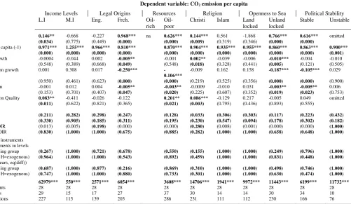
14 Table 1: Environmental Unsustainability with CO2 emissions per capita

Dependent variable: CO2 emission per capita

Income Levels Legal Origins Resources Religion Openness to Sea Political Stability

L.I M.I Eng. Frch.

Oil-rich Oil-poor

Christi Islam Land

locked

Unland locked

Stable Unstable

Constant 0.146** -0.668 -0.227 0.968*** na 0.626*** 0.144*** 0.561 -1.868 0.766*** 0.616*** omitted

(0.034) (0.775) (0.449) (0.000) (0.000) (0.009) (0.319) (0.346) (0.000) (0.000)

CO2 per capita (-1) 0.971*** 1.255*** 0.966*** 0.810*** 0.870*** 0.904*** 0.935*** 0.955*** 0.860*** 0.863*** 0.900***

(0.000) (0.000) (0.000) (0.000) (0.000) (0.000) (0.000) (0.000) (0.000) (0.000) (0.001)

GDP growth -0.0004 -0.044 0.002 -0.005** -0.001 0.002** -0.039 -0.006 -0.010*** -0.004 -0.010 (0.548) (0.389) (0.668) (0.049) (0.548) (0.018) (0.328) (0.441) (0.005) (0.121) (0.505) Population growth 0.001 0.308 0.017 -0.250***

-0.106***

-0.009 0.162 0.158 -0.187*** -0.105*** 0.029 (0.950) (0.461) (0.623) (0.000) (0.000) (0.219) (0.525) (0.356) (0.000) (0.000) (0.900) Education -0.001 0.012 0.004 -0.005** -0.003** -0.0009 -0.010 0.031 -0.003** -0.005** 0.006

(0.153) (0.701) (0.407) (0.047) (0.020) (0.225) (0.607) (0.352) (0.019) (0.023) (0.753) Regulation Quality 0.083** -0.411 -0.026 -0.122 0.201** 0.086*** -0.129 0.217 -0.005 0.049 omitted

(0.011) (0.622) (0.821) (0.365) (0.021) (0.003) (0.795) (0.436) (0.893) (0.555)

AR(1) (0.211) (0.282) (0.298) (0.247) (0.128) (0.033) (0.306) (0.303) (0.117) (0.223) (0.432)

AR(2) (0.330) (0.905) (0.185) (0.311) (0.195) (0.230) (0.547) (0.094) (0.178) (0.302) (0.182)

Sargan OIR (0.013) (0.005) (0.198) (0.000) (0.000) (0.280) (0.008) (0.001) (0.000) (0.000) (1.000)

Hansen OIR (0.830) (1.000) (1.000) (0.675) (0.885) (0.282) (1.000) (1.000) (0.658) (0.648) (1.000)

DHT for instruments (a)Instruments in levels

H excluding group (0.267) (1.000) (0.721) (0.678) (0.550) (0.155) (1.000) (1.000) (0.249) (0.796) (1.000)

Dif(null, H=exogenous) (0.964) (1.000) (1.000) (0.543) (0.892) (0.459) (1.000) (1.000) (0.831) (0.448) (1.000)

(b) IV (years, eq(diff))

H excluding group (0.687) (1.000) (0.877) (0.216) (0.869) (0.310) (1.000) (1.000) (0.498) (0.746) (1.000)

Dif(null, H=exogenous) (0.747) (1.000) (1.000) (0.880) (0.733) (0.301) (1.000) (1.000) (0.630) (0.474) (1.000)

Fisher 62979*** 550*** 2571*** 6054*** 3608*** 14706*** 1941*** 9972*** 11443*** 6199*** 11732***

Instruments 28 28 28 28 28 28 28 28 28 28 28 Countries 29 15 17 27 37 30 14 14 30 34 10 Observations 227 115 139 203 286 231 111 112 230 166 76

LI: Low Income countries. MI: Middle Income countries. Eng: English Common law countries. Frch: French Civil law countries. Oil-rich: Oil exporting countries. Oil-poor: Nonoil exporting countries. Christ: Christian-dominated countries. Islam: Islam-dominated countries. Landlocked: Landlocked countries. Unlandlocked: Unlandlocked countries. Stable: Politically stable countries. Unstable: Politically unstable

countries. *,**,***: significance levels of 10%, 5% and 1% respectively. DHT: Difference in Hansen Test for Exogeneity of Instruments’

Subsets. Dif: Difference. OIR: Over-identifying Restrictions Test. The significance of bold values is twofold. 1) The significance of estimated coefficients and the Fisher statistics. 2) The failure to reject the null hypotheses of: a) no autocorrelation in the AR(1) and AR(2) tests and; b) the validity of the instruments in the Sargan and Hansen OIR tests.

The following can be established for the remaining five hypotheses. (i) Hypothesis 1

postulating that middle income countries have a lower level of persistence in CO2 emissions is

valid in Tables 1 (CO2 per capita emissions), Table 2 (CO2 emissions from electricity and heat

production) and Table 3 (CO2 emissions from liquid fuel consumption). (ii) Hypothesis 2 on the

edge of French civil law countries is valid in Table 3 (CO2 emissions from liquid fuel

consumption) and Table 4 (CO2 intensity), but not in Table 1 (CO2 per capita emissions). (iii)

Hypothesis 3 on the postulation that politically-unstable countries reflect more persistence is

valid in Table 1 (CO2 per capita emissions). (iv) Hypothesis 5 on the propensity for landlocked

countries to be associated with more persistence in CO2 emissions is valid in Table 1 (CO2 per

capita emissions) but not in Table 3 (CO2 emissions from liquid fuel consumption). (v)

Hypothesis 6 maintaining that Christianity-dominated countries are more environmentally

friendly with regard to CO2 emissions is valid in Table 1 (CO2 per capita emissions) but not in

(16)

15 Table 2: Environmental Unsustainability CO2 emissions from electricity and heat

production

Dependent variable: CO2 emissions from electricity and heat production

L.I M.I Eng. Frch.

Oil-rich

Oil-poor Christi Islam Land

locked

Unland locked

Stable Unstable

Constant -11.209 omitted omitted 3.473 na 7.095 3.101 na na -7.242 -7.519 na (0.457) (0.768) (0.637) (0.745) (0.557) (0.627) CO2 emissions (-1) 0.985*** 1.130*** 1.132*** 1.008*** 0.892*** 1.079*** 1.033*** 1.018***

(0.000) (0.000) (0.000) (0.000) (0.000) (0.000) (0.000) (0.000)

GDP growth 0.434 -0.150 0.144 0.067 0.259 0.212 0.129 0.032 (0.227) (0.579) (0.522) (0.503) (0.255) (0.436) (0.311) (0.869) Population growth -2.287 -3.122 -0.576 2.430 -0.441 -1.127 -0.278 0.630

(0.288) (0.768) (0.861) (0.764) (0.886) (0.607) (0.959) (0.755) Education 0.282 0.112 -0.135 -0.156 0.010 -0.034 0.057 0.028

(0.322) (0.827) (0.309) (0.327) (0.971) (0.860) (0.665) (0.901) Regulation Quality omitted omitted -3.791 -1.438 11.175 -0.248 -6.119 -1.925

(0.499) (0.789) (0.327) (0.955) (0.191) (0.850) AR(1) (0.082) (0.499) (0.192) (0.240) (0.103) (0.240) (0.003) (0.109) AR(2) (0.147) (0.386) (0.348) (0.662) (0.154) (0.462) (0.265) (0.125)

Sargan OIR (0.985) (0.322) (1.000) (0.885) (0.919) (0.968) (0.950) (0.981)

Hansen OIR (1.000) (1.000) (0.763) (1.000) (1.000) (1.000) (1.000) (1.000)

H excluding group (1.000) (1.000) (1.000) (1.000) (0.103) (0.943) (0.772) (0.844)

Dif(null, H=exogenous)

(1.000) (1.000) (1.000) (1.000) (0.154) (1.000) (1.000) (1.000)

(1.000) (1.000) (1.000) (1.000) (1.000) (1.000) (1.000) (1.000)

Fisher 177.20*** 1666*** 284*** 8908*** 107.10*** 47844*** 345.50*** 52.89***

Instruments 28 28 28 28 28 28 28 28 Countries 14 8 8 14 18 16 18 17 Observations 106 63 69 100 142 120 144 139

[image:16.595.42.553.126.432.2]

(17)

16 Table 3: Environmental Unsustainability with CO2 emissions from liquid fuel

consumption

Dependent variable: CO2 emissions from liquid fuel consumption

L.I M.I Eng. Frch.

Oil-rich

locked

Unland locked

Stable Unstable

Constant 0.494 -121.84 -1.140 7.817*** na 0.856 1.476 omitted 197.928* 0.447 0.011 n.a (0.848) (0.326) (0.861) (0.006) (0.809) (0.622) (0.068) (0.871) (0.998) CO2 emissions (-1) 0.873*** 2.249 1.125*** 0.902*** 0.964*** 0.907*** 1.430** -2.658 0.970*** 0.956***

(0.000) (0.100) (0.000) (0.000) (0.000) (0.000) (0.029) (0.158) (0.000) (0.000)

GDP growth -0.115*** -0.189 -0.381* -0.014 -0.024 -0.034 2.813 -1.743** -0.028 -0.019

(0.004) (0.222) (0.073) (0.558) (0.661) (0.477) (0.505) (0.040) (0.556) (0.716)

Population growth 3.223*** 7.800 1.284 0.337 0.892** 0.843 -4.907 17.049** 0.393* 0.439**

(0.000) (0.294) (0.286) (0.149) (0.013) (0.140) (0.541) (0.031) (0.070) (0.048)

Education 0.020 0.734 -0.054 0.019 0.032 0.112*** -0.785 1.501** 0.010 0.054 (0.519) (0.286) (0.839) (0.297) (0.428) (0.002) (0.450) (0.045) (0.731) (0.172) Regulation Quality -1.125 13.870 2.169 1.715 1.662 0.866 -36.182 0.648 1.639* 0.060

(0.460) (0.528) (0.784) (0.248) (0.323) (0.543) (0.435) (0.833) (0.095) (0.972) AR(1) (0.012) (0.656) (0.133) (0.051) (0.005) (0.007) (0.548) (0.207) (0.010) (0.006) AR(2) (0.049) (0.984) (0.218) (0.192) (0.027) (0.029) (0.590) (0.165) (0.032) (0.034) Sargan OIR (0.925) (0.306) (0.968) (0.898) (0.694) (0.864) (0.122) (0.317) (0.949) (0.753)

Hansen OIR (0.822) (1.000) (0.997) (0.743) (0.771) (0.890) (1.000) (1.000) (0.882) (0.305)

H excluding group (0.369) (1.000) (0.785) (0.608) (0.640) (0.879) (1.000) (1.000) (0.410) (0.551)

(0.909) (1.000) (0.997) (0.670) (0.689) (0.736) (1.000) (1.000) (0.947) (0.213)

H excluding group (0.922) (1.000) (0.918) (0.931) (0.641) (0.464) (1.000) (1.000) (0.837) (0.163)

(0.596) (1.000) (0.985) (0.481) (0.688) (0.933) (1.000) (1.000) (0.747) (0.483)

Fisher 714.16*** 45.32*** 192.11*** 412.22*** 270.10*** 1324*** 481468*** 137.26*** 1129*** 197.08***

Instruments 28 28 28 28 28 28 28 28 28 28 Countries 29 15 17 27 37 30 14 14 30 34 Observations 227 115 139 203 286 231 11 112 230 266

[image:17.595.38.560.112.415.2]

(18)

[image:18.595.43.563.108.413.2]

17 Table 4: Environmental Unsustainability with CO2 intensity (kg of oil equivalent energy

use)

Dependent variable: CO2 intensity

L.I M.I Eng. Frch.

Oil-rich

locked

Unland locked

Stable Unstable

Constant 0.530 na omitted 0.276 0.117 0.097 omitted na -0.151 0.416 na (0.899) (0.535) (0.893) (0.924) (0.900) (0.644) CO2 emissions (-1) 0.926*** 0.123 0.900*** 0.978*** 0.975*** 1.186*** 0.975*** 0.974***

(0.001) (0.890) (0.000) (0.000) (0.000) (0.000) (0.000) (0.000)

GDP growth 0.017 0.369 0.006 0.002 -0.005 -0.004 -0.005 -0.001 (0.849) (0.352) (0.519) (0.909) (0.862) (0.658) (0.866) (0.909) Population growth -0.231 -6.323 -0.144** 0.034 -0.171 -0.945 -0.062 -0.196

(0.902) (0.378) (0.035) (0.976) (0.790) (0.284) (0.934) (0.707) Education -0.003 0.370 0.002 -0.004 0.009 0.032 0.011 0.003

(0.941) (0.372) (0.617) (0.945) (0.748) (0.300) (0.738) (0.899) Regulation Quality -0.442 9.421 -0.111 0.119 -0.044 -1.140 0.145 0.142

(0.850) (0.353) (0.504) (0.892) (0.953) (0.312) (0.838) (0.830) AR(1) (0.822) (0.246) (0.106) (0.593) (0.844) (0.280) (0.453) (0.331)

AR(2) (0.823) (0.289) (0.410) (0.971) (0.897) (0.762) (0.844) (0.550)

Sargan OIR (0.000) (0.000) (0.364) (0.000) (0.000) (0.223) (0.000) (0.000) Hansen OIR (1.000) (1.000) (0.993) (1.000) (1.000) (1.000) (1.000) (1.000)

(1.000) (1.000) (1.000) (1.000) (1.000) (1.000) (0.996) (0.997)

(1.000) (1.000) (1.000) (1.000) (1.000) (1.000) (1.000) (1.000)

Fisher 69.46*** 161.99*** 246.46*** 30174*** 82521*** 862582*** 12474*** 18901***

Instruments 28 28 28 28 28 28 28 28 Countries 19 10 21 26 21 10 25 26 Observations 115 74 115 159 133 56 159 159

Subsets. Dif: Difference. OIR: Over-identifying Restrictions Test. The significance of bold values is twofold. 1) The significance of estimated coefficients and the Fisher statistics. 2) The failure to reject the null hypotheses of: a) no autocorrelation in the AR(1) and AR(2) tests and; b) the validity of the instruments in the Sargan and Hansen OIR tests.

5. Concluding implications, caveats and future research directions

Motivated by sustainable development challenges in Sub-Saharan Africa, this study has

assessed the comparative persistence in environmental unsustainability in a sample of 44

countries in the sub-region for the period 2000 to 2012. The empirical evidence is based on

Generalised Method of Moments. The dataset is decomposed into fundamental characteristics

of environmental degradation based on income levels (low income versus (vs.) middle income

countries); legal origins (English Common law vs. French Civil law countries); religious

domination (Christianity- vs. Islam-dominated countries); openness to sea (landlocked vs.

coastal countries); resource-wealth (oil-rich vs. oil-poor countries) and political stability (stable

vs. unstable countries).

Of the six hypotheses tested, it is not feasible to assess the hypothesis on

(19)

18 findings have been established. (i) Hypothesis 1 postulating that middle income countries have

a lower level of persistence in CO2 emissions is valid for CO2 per capita emissions, CO2

emissions from electricity and heat production and CO2 emissions from liquid fuel

consumption. (ii) Hypothesis 2 on the edge of French Civil law countries is valid for CO2

emissions from liquid fuel consumption and CO2 intensity, but not for CO2 per capita

emissions. (iii) Hypothesis 3 on the postulation that politically-unstable countries reflect more

persistence is valid for CO2 per capita emissions. (iv) Hypothesis 5 on the propensity for

landlocked countries to be associated with more persistence in CO2 emissions is valid for CO2

per capita emissions but not for CO2 emissions from liquid fuel consumption. (v) Hypothesis 6

maintaining that Christian-dominated countries are more environmentally friendly with regard

to CO2 emissions is valid for CO2 per capita emissions but not for CO2 emissions from liquid

fuel consumption and CO2 intensity. Before discussing policy and theoretical implications, we

clarify Hypothesis 6 for which corresponding findings on its invalidity outweigh results for its

validity.

We have postulated that since Christianity-dominated countries are more open to the

neoliberal culture, it is more likely that they have better institutions that manage the

environment more sustainably than their Islam-oriented counterparts. Unfortunately, this

hypothesis has been rejected by a substantial margin (two of the three CO2 emissions

variables). Upon more intuition, what we have overlooked in the establishment of the testable

hypotheses is the fact that nations which are more liberal are also more likely to adopt

capitalistic tendencies that are not friendly to sustainable development (Roudometof, 2014).

This interpretation and clarification are broadly consistent with Obeng-Odoom (2015). The

author, in a critique of the ‘Africa rising’ narrative has argued that neoliberal policies imposed

on Africa are more focused on increasing the relevance of capital accumulation, with less

concern on more fundamental ethnical issues like environmental degradation and inequality.

Moreover, liberal economies are generally more opened and there is an established relationship

between openness and the carbon footprint of countries (Peters & Hertwich, 2008; Hertwich &

Peters, 2009).

The main policy implication is that, contingent on comparative persistence in CO2

emissions, more resources can be devoted to addressing the policy syndrome within a

fundamental characteristic. It is important to note that persistence in a negative aspect of

environmental quality represents a policy syndrome. Such persistence implies that past CO2

emissions positively affect future CO2 emissions. Furthermore, more persistence in one

(20)

19 emissions have a more proportionate impact on future CO2 emissions in the sub-panel

exhibiting more persistence.

The theoretical contribution of this study builds on the established persistence in

negative economic signals. By deviating from mainstream convergence literature which is

based on catch-up in per capita income (or positive economic signals), we have shown in this

study that the theoretical underpinnings of the convergence literature can be extended to

negative signals. This theoretical extension is consistent with a recent stream of literature on

policy harmonization based on catch-up in policy syndromes, namely: the prediction of the

Arab Spring based on negative governance and macroeconomic signals (Asongu &

Nwachukwu, 2016d) and the fight against capital flight (Asongu, 2014). Therefore, these

findings should also be viewed through the lens of a theory-building exercise because applied

econometrics should not be exclusively based on the acceptance or rejection of existing

theoretical underpinnings. Accordingly, the underpinnings of an existing theory can be

employed in other development fields. In essence, we have built on the theoretical

underpinnings of income convergence literature (Barro, 1991; Barro & Sala-i-Martin, 1992,

1995; Mankiw et al., 1992; Baumol, 1986) to assess persistence in environmental degradation.

This improves recent theoretical literature on the need to extend the theoretical underpinnings

of income convergence to other development fields, notably: financial market development

(Narayan et al., 2011; Bruno et al., 2012) and inclusive human development (Mayer-Foulkes,

2010; Asongu & Nwachukwu, 2017a). Moreover, the attendant literature has fundamentally

been based on positive macroeconomic signals. In this study, the variables used on

environmental degradation are negative macroeconomic signals because the persistence in

negative macroeconomic signals may even require more policy intervention, compared to the

persistence of positive macroeconomic signals.

Two main caveats are worth discussing, notably: the contingency of the analysis on the

choice of variables employed and assumptions underlying the testable hypotheses. The points

are expanded chronological order. First, as highlighted in the data section, it is impossible to

use all the CO2 emission variables from the World Bank Development database. Hence, we

have been limited to a selected few based on constraints in missing observations in the other

variables. It follows that the established evidence of persistence is contingent on the outcome

variables as well as the variables used in the conditioning information set. This contingency of

results in the variables employed in the model is a fundamental shortcoming of conditional (or

contingent) convergence and/or persistence modelling by means of the Generalised of the

(21)

20 Second, some of the motivations underpinnings the postulated hypotheses may be

problematic. For instance, critics of the assumption underpinning the legal origin hypothesis

maintain that the strength of British Common law vis-à-vis French Civil law may not hold for a

plethora of reasons (Deakin & Siems 2010; Fowowe, 2014; Asongu, 2015). (i) It is doubted in

some scholarly circles whether the distinction between Civil law and Common law is justifiable

from a historical standpoint. (ii) With internationalization in the contemporary era, the

distinction between Civil law and Common law is less persuasive. (iii) The categorization of

countries in terms of Civil law and Common law does not take into account the following

factors, inter alia: modifications and mixtures at the moment foreign laws were copied by

former colonies, the influence of transplant law and the post-transplant period during which the

law transplanted could still be altered or applied differently. Notwithstanding these caveats, we

do not expect the hypotheses to be 100% accurate, which is the reason an empirical exercise is

needed to either validate or reject them.

Future research can improve the extant literature by investigating whether the

established linkages withstand empirical scrutiny when other regions of the world are

investigated. It would also be interesting to assess the probability of occurrence of established

(22)

21 Appendices

Appendix 1: Variable Definitions

Variables Signs Variable Definitions (Measurement) Sources

CO2 per capita CO2mtpc CO2 emissions (metric tons per capita) World Bank

(WDI) CO2 from electricity

and heat

CO2elehepro CO2 emissions from electricity and heat production, total

(% of total fuel combustion)

World Bank (WDI) CO2 from liquid

fuel

CO2lfcon CO2 emissions from liquid fuel consumption (% of total) World Bank

(WDI) CO2 intensity CO2inten CO2 intensity (kg per kg of oil equivalent energy use) World Bank

(WDI) Educational Quality Educ Pupil teacher ratio in Primary Education World Bank

(WDI) GDP growth GDPg Gross Domestic Product (GDP) growth (annual %) World Bank

(WDI) Population growth Popg Population growth rate (annual %) World Bank

(WDI)

Regulation Quality RQ

“Regulation quality (estimate): measured as the ability of the government to formulate and implement sound policies and regulations that permit and promote private sector development”

World Bank (WDI)

WDI: World Bank Development Indicators.

Appendix 2: Summary statistics (2000-2012)

Mean SD Minimum Maximum Observations

CO2 per capita 0.901 1.820 0.016 10.093 567

CO2 from electricity and heat 23.730 18.870 0.000 71.829 286

CO2 from liquid fuel 78.880 23.092 0.000 100 567

CO2 intensity 2.044 6.449 0.058 77.586 321

Educational Quality 43.784 14.731 12.466 100.236 425 GDP growth 4.851 5.000 -32.832 33.735 567 Population growth 2.334 0.866 -1.081 6.576 529 Regulation Quality -0.607 0.544 -2.238 0.983 530

S.D: Standard Deviation.

Appendix 3: Correlation matrix (uniform sample size: 155 )

CO2mtpc CO2elehepro CO2lfcon CO2inten Educ GDPg Popg RQ

1.000 0.690 -0.721 0.805 -0.369 -0.057 -0.611 0.593 CO2mtpc

1.000 -0.695 0.703 -0.502 -0.052 -0.524 0.505 CO2elehepro

1.000 -0.551 0.246 0.020 0.364 -0.366 CO2lfcon

1.000 -0.509 -0.055 -0.698 0.676 CO2inten

1.000 0.104 0.515 -0.515 Educ

1.000 0.074 -0.140 GDPg

1.000 -0.624 Popg

1.000 RQ

CO2mtpc: CO2 emissions (metric tons per capita). CO2elehepro: CO2 emissions from electricity and heat production, total

(% of total fuel combustion). CO2lfcon: CO2 emissions from liquid fuel consumption (% of total). CO2inten: CO2 intensity

(23)

22

Appendix 4: Categorization of Countries

Categories Panels Countries Num

Income levels

Middle Income

Algeria, Angola, Botswana, Cameroon, Cape Verde, Côte d’Ivoire, Egypt,

Equatorial Guinea, Gabon, Lesotho, Libya, Mauritius, Morocco, Namibia, Nigeria, , Senegal, Seychelles, South Africa, Sudan, Swaziland, Tunisia.

21

Low Income

Benin, Burkina Faso, Burundi, Central African Republic, Chad, Comoros, Congo Democratic Republic, Congo Republic, Djibouti, Eritrea, Ethiopia, The Gambia, Ghana, Guinea, Guinea-Bissau, Kenya, Liberia, Madagascar, Malawi, Mali, Mauritania, Mozambique, Niger, Rwanda, Sierra Leone, Somalia, Togo, Uganda, Zambia, Zimbabwe. 30 Legal Origins English Common-law

Botswana, The Gambia, Ghana, Kenya, Lesotho, Liberia, Malawi, Mauritius, Namibia, Nigeria, Seychelles, Sierra Leone, Somalia, South Africa, Sudan, Swaziland, Uganda, Zambia, Zimbabwe.

19

French Civil-law

Algeria, Angola, Benin, Burkina Faso, Burundi, Cameroon, Cape Verde, Central African Republic, Chad, Comoros, Congo Democratic Republic, Congo Republic,

Côte d’Ivoire, Djibouti, Egypt, Equatorial Guinea, Eritrea, Ethiopia, Gabon, Guinea,

Guinea-Bissau, Libya, Madagascar, Mali, Mauritania, Morocco, Mozambique, Niger, Rwanda, Senegal, Togo, Tunisia.

32

Religion

Christianity Angola, Benin, Botswana, Burundi, Cameroon, Cape Verde, Central African

Republic, Congo Democratic Republic, Congo Republic, Côte d’Ivoire, Equatorial

Guinea, Eritrea, Ethiopia, Gabon, Ghana, Kenya, Lesotho, Liberia, Madagascar, Malawi, Mauritius, Mozambique, Namibia, Rwanda, Seychelles, South Africa, South Africa, Togo, Uganda, Zambia, Zimbabwe.

31

Islam Algeria, Burkina Faso, Chad, Comoros, Djibouti, Egypt, The Gambia, Guinea, Guinea Bissau, Libya , Mali, Mauritania, Morocco, Niger, Nigeria, Senegal, Sierra Leone, Somalia, Sudan, Tunisia,

20

Resources

Petroleum Exporting

Algeria, Angola, Cameroon, Chad, Congo Republic, Equatorial Guinea, Gabon, Libya, Nigeria, Sudan.

10

Non-Petroleum Exporting

Benin, Botswana, Burkina Faso, Burundi, Cape Verde, Central African Republic,

Comoros, Congo Democratic Republic, Côte d’Ivoire, Djibouti, Eritrea, Ethiopia,

Egypt, The Gambia, Ghana, Guinea, Guinea-Bissau, Kenya, Lesotho, Liberia, Madagascar, Malawi, Mali, Mauritania, Mauritius, Morocco, Mozambique, Namibia, Niger, Senegal, Sierra Leone, Somalia, Rwanda, Seychelles, South Africa, Swaziland, Togo, Tunisia, Uganda, Zambia, Zimbabwe.

41

Stability

Conflict Angola, Burundi, Chad, Central African Republic, Congo Democratic Republic,

Côte d’Ivoire, Liberia, Nigeria, Sierra Leone, Somalia, Sudan, Zimbabwe. 12

Non-Conflict

Algeria, Benin, Botswana, Burkina Faso, Cameroon, Cape Verde, Comoros, Congo Republic, Djibouti, Egypt, Equatorial Guinea, Eritrea, Ethiopia, Gabon, The Gambia, Ghana, Guinea, Guinea-Bissau, Kenya, Lesotho, Libya, Madagascar, Malawi, Mali, Mauritania, Mauritius, Morocco, Mozambique, Namibia, Niger, Senegal, Rwanda, Seychelles, South Africa, Swaziland, Togo, Tunisia, Uganda, Zambia.

39

Openness to Sea

Landlocked Botswana, Burkina Faso, Burundi, Chad, Central African Republic, Ethiopia, Lesotho, Malawi, Mali, Niger, Rwanda, Swaziland, Uganda, Zambia, Zimbabwe

15

Not landlocked

Algeria, Angola, Benin, Cameroon, Cape Verde, Comoros, Congo Democratic

Republic, Congo Republic, Côte d’Ivoire, Djibouti, Egypt, Equatorial Guinea,

Eritrea, Gabon, The Gambia, Ghana, Guinea, Guinea-Bissau, Kenya, Liberia, Libya, Madagascar, Mauritania, Mauritius, Morocco, Mozambique, Namibia, Nigeria, Senegal, Sierra Leone, Somalia, Sudan, Seychelles, South Africa, Togo, Tunisia.

36

(24)

23 References

Agbor, J. A. (2015). “How does colonial origin matter for economic performance in sub-

Saharan Africa?”, In Augustin K. Fosu (Ed.), Growth and Institutions in African Development,

Chapter 13, pp. 309-327, Routledge Studies in Development Economics: New York.

Akbostanci, E., S. Turut-Asi & Tunc, G. I., (2009). “The Relationship between Income and

Environment in Turkey: Is there an Environmental Kuznets Curve?”, Energy Policy, 37(3), pp. 861-867.

Akinlo, A. E., (2008). “Energy consumption and economic growth: evidence from 11 Sub -Sahara African countries”. Energy Economics, 30(5), pp. 2391–2400.

Akinyemi, O., Alege, P., Osabuohien, E., & Ogundipe, A., (2015). “Energy Security and the Green Growth Agenda in Africa: Exploring Trade-offs and Synergies”, Department of

Economics and Development Studies, Covenant University, Nigeria.

Akpan, G. E. & Akpan, U. F. (2012). “Electricity Consumption, Carbon Emissions and

Economic Growth in Nigeria”, International Journal of Energy Economics and Policy, 2(4), pp. 292-306.

Amavilah, V. H. (2015). “Social Obstacles to Technology, Technological Change, and the Economic Growth of African Countries: Some Anecdotal Evidence from Economic History”,

MPRA Paper No. 63273, Munich.

Amavilah, V., Asongu, S. A., & Andrés, A. R., (2017). “Effects of globalization on peace and stability: Implications for governance and the knowledge economy of African countries”,

Technological Forecasting and Social Change, 122 (September), pp. 91-103.

America, R., (2013). “Economic Development with Limited Supplies of Management. What to do about it - the case of Africa”, Challenge, 56(1), pp. 61-71.

Ang, J. B. (2007). “CO2 emissions, energy consumption, and output in France”, Energy Policy, 35(10), pp. 4772-4778.

Anyangwe, E. (2014). “Without energy could Africa’s growth run out of steam?” theguardian,

http://www.theguardian.com/global-development-professionals-network/2014/nov/24/energy-infrastructure-clean-cookstoves-africa (Accessed: 08/09/2015).

Anyanwu, J., & Erhijakpor, A., (2014). “Does Oil Wealth Affect Democracy in Africa?”African Development Review, 26 (1), pp. 15-37.

Apergis, N. & J. Payne, J. E., (2009). “CO2 emissions, energy usage, and output in Central

America”, Energy Policy, 37(8), pp. 3282-3286.

Arvis, J-F., Marteau, J-F., & Raballand, G. (2007). The cost of being landlocked: logistics

costs and supply chain reliability”, Word Bank Working Paper Series No. 4258, Washington.