Extracting token level signals of syntactic processing from fMRI with an application to PoS induction

Extracting token-level signals of syntactic processing from fMRI - with an

application to PoS induction

Joachim Bingel Maria Barrett Anders Søgaard

Centre for Language Technology, University of Copenhagen Njalsgade 140, 2300 Copenhagen S, Denmark

{bingel, barrett, soegaard}@hum.ku.dk

Abstract

Neuro-imaging studies on reading differ-ent parts of speech (PoS) report somewhat mixed results, yet some of them indicate different activations with different PoS. This paper addresses the difficulty of using fMRI to discriminate between linguistic tokens in reading of running text because of low temporal resolution. We show that once we solve this problem, fMRI data contains a signal of PoS distinctions to the extent that it improves PoS induction with error reductions of more than 4%.

1 Introduction

A few recent studies have tried to extract mor-phosyntactic signals from measurements of human sentence processing and used this information to improve NLP models. Klerke et al. (2016), for ex-ample, used eye-tracking recordings to regularize a sentence compression model. More related to this work, Barrett et al. (2016) recently used eye-tracking recordings to induce PoS models. How-ever, a weakness of eye-tracking data is that while eye movement surely does reflect the temporal as-pect of cognitive processing, it is only a proxy of the latter and does not directly represent which processes take place in the brain.

A recent neuro-imaging study suggests that concrete nouns and verbs elicit different brain sig-natures in the frontocentral cortex, and that con-crete and abstract nouns elicit different brain acti-vation patterns (Moseley and Pulverm¨uller, 2014). Also, for example, concrete verbs activate motor and premotor cortex more strongly than concrete nouns, and concrete nouns activate inferior frontal areas more strongly than concrete verbs. A decade earlier, Tyler et al. (2004) showed that the left in-ferior frontal gyrus was more strongly activated in

processing regularly inflected verbs compared to regularly inflected nouns.

Such studies suggest that different parts of our brains are activated when reading different parts of speech (PoS). This would in turn mean that neuro-images of readers carry information about the grammatical structure of what they read. In other words, neuro-imaging provides a partial, noisy annotation of the data with respect to mor-phosyntactic category.

Say neuro-imaging data of readers was readily available. Would it be of any use to, for exam-ple, engineers interested in PoS taggers for low-resource languages? This is far from obvious. In fact, it is well-known that neuro-imaging data from reading is noisy, in part because the reading signal is not always very distinguishable (Taga-mets et al., 2000), and also because the content of what we read may elicit certain activation in brain regions e.g. related to sensory processing (Boulenger et al., 2006; Gonz´alez et al., 2006).

Other researchers such as Borowsky et al. (2013) have also questioned that there are differ-ences, claiming to show that the majority of acti-vation is shared between nouns and verbs – includ-ing in regions suggested by previous researchers as unique to either nouns or verbs. Berlingeri et al. (2008) argue that only verbs could be associ-ated with unique regions, not nouns.

In this paper we nevertheless explore this ques-tion. The paper should be seen as a proof of con-cept that interesting linguistic signals can be ex-tracted from brain imaging data, and an attempt to show that learning NLP models from such data could be a way of pushing the boundaries of both fields.

Contributions (a) We present a novel technique for extracting syntactic processing signal at the to-ken level from neuro-imaging data that is

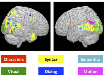
Figure 1: Neural activity by brain region and type of information processed, as measured and ren-dered by Wehbe et al. (2014).

terized by low temporal resolution. (b) We demon-strate that the fMRI data improves performance of a type-constrained, second order hidden Markov model for PoS induction. Our model leads to an error reduction of more than 4% in tagging accu-racy despite very little training data, which to the best of our knowledge is the first positive result on weakly supervised part-of-speech induction from fMRI data in the literature.

2 fMRI

Functional Magnetic Resonance Imaging (fMRI) is a technology for spatial visualization of brain activity. It measures the changes in oxygenation of the blood in the brain, often by use of the blood oxygenation level-dependent contrast (Ogawa et al., 1992), which correlates with neural activity. While the spatial resolution of fMRI is very high, its temporal resolution is low compared to other brain imaging technologies like EEG, which usu-ally returns millisecond records of brain activity, but on the contrary have low spatial resolution. The temporal resolution of fMRI is usually be-tween 0.5Hz and 1Hz. fMRI data contains rep-resentations of neural activity of millimeter-sized cubes calledvoxels.

The high spatial resolution may enable us to de-tect fine differences in brain activation patterns, such as between processing nouns and verbs, but the low temporal resolution is a real challenge when the different tokens are processed serially and quickly after each other, as is the case in read-ing.

Another inherent challenge when working with

fMRI data is the lag between the the reaction to a stimulus and the point when it becomes visi-ble through fMRI. This lag is called the hemo-dynamic response latency. While we know from brain imaging technologies with higher tempo-ral resolution that the neutempo-ral response to a stim-uli happens within milliseconds, it only shows in fMRI data after a certain period of time, which further blurs the low temporal dimension of se-rial fMRI recordings. This latency has been stud-ied as long as fMRI technology itself. It depends on the blood vessels and varies between e.g. vox-els, brain regions, subjects, and tasks. A meta study of the hemodynamic response report laten-cies between 4 and 14 seconds in healthy adults, though latencies above 11 seconds are less typi-cally reported (Handwerker et al., 2012). Accord-ing to Handwerker et al. (2012), the precise re-sponse shape for a given stimulus and voxel region is hard to predict and remains a challenge when modeling temporal aspects of fMRI data.

Figure 1 visualizes the neural activations in different brain regions as a reaction to the type of information that is processed during reading. See Price (2012) for a thorough review of fMRI language studies.

Wehbe et al. (2014) presented a novel approach to fMRI studies of linguistic processing by study-ing a more naturalistic readstudy-ing scenario, and mod-eling the entire process of reading and story un-derstanding. They used data from 8 subjects read-ing contextualized, runnread-ing text: a chapter from a Harry Potter book. The central benefit of this approach is that it allows studies of complex text processing closer to a real-life reading experi-ence. Wehbe et al. (2014) used this data to train a comprehensive, generative model that—given a text passage—could predict the fMRI-recorded activity during the reading of this passage. Us-ing the same data, our goal is to model a specific aspect of the story understanding process, i.e. the grammatical processing of words.

3 Data

3.1 Textual data

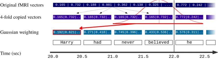
sep-Figure 2: Computation of token-level fMRI vectors from the original fMRI data for the first token “Harry” while accounting for hemodynamic response latency using a Gaussian sliding window over a certain time window (indicated by red horizontal line). The final fMRI vector for “Harry” (red box) is computed as specified in Equation 1. In this example, the time stamptfor the token is20sand the time window stretches fromt+ 1stot+ 2.5s.

arated from the tokens at the end of clauses and sentences. As the temporal alignment between to-kens and fMRI recordings (see below) forbids us to detach punctuation marks from their preceding tokens and introduce them as new tokens, we opt to remove all punctuation from the data. In the same process, we use simple heuristics to detect sentence boundaries. Finally, we correct errors in sentence splitting manually.

The chapter counts 4,898 tokens (excluding punctuation) and 1,411 types in 408 sentences.

3.2 fMRI data

The fMRI data from the same data set is available as high-dimensional vectors of flattened third-order tensors, in which each component represents the blood-oxygen-level dependent contrast for a certain voxel in the three-dimensional fMRI im-age. The resolution of the image is at3×3×3mm, such that the brain activity for the eight subjects is represented by approximately 31,400 voxels on average (standard deviation is 3,607) depending on the size of their brain.

This data is recorded every two seconds during the reading process, in which each token is con-secutively displayed for 0.5 seconds on a screen inside the fMRI scanner. Prior to reading, the sub-jects are asked to focus on a cross displayed at the center of the screen in a warm-up phase of 20 seconds. The chapter is divided into four blocks, separated by additional concentration phases of 20 seconds. Furthermore, paragraphs are separated by a 0.5-seconds display of a cross at the center of the screen.

As mentioned in the preceding section, punc-tuation marks were not displayed separately, but instead attached to the preceding token. This is arguably motivated through the attempt to create a reading scenario that is as natural as possible within the limitations of an fMRI recording. In similar fashion, contractions such asdon’torhe’s were represented as one token, just as they appear in the original text.

In order to make the data feasible for our HMM approach (see Section 4), we apply Principal Com-ponent Analysis (PCA) to the high-dimensional fMRI vectors. We initially tune the number of principal components, which we describe in Sec-tion 5.

3.2.1 Computing token-level fMRI vectors

As outlined above, the time resolution of the fMRI recordings means that every block of four consecutive tokens is time-aligned with a single fMRI image. Naturally, this shared representa-tion of consecutive tokens complicates any lan-guage learning at the token level. Furthermore, the hemodynamic response latency inherent to fMRI recordings entails that the image recorded while reading a certain token most probably does not give any clues about the mental state elicited by this stimulus.

We therefore face the dual challenge of

1. inferring token-level information from supra-token recordings, and

zi-2 zi-1 zi

xi-2 xi-1 xi

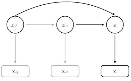
Figure 3: Second-order HMM incorporating tran-sitional probabilities from first and second-degree preceding states.

We address this problem through the follow-ing procedure that we illustrate in Figure 2. First, we copy the number of fMRI recordings fourfold, such that every fMRI vector is aligned to exactly one token (excluding the vectors that are recorded while no token was displayed). The representation for a given token is then computed as a weighted average over all fMRI vectors that lie within a cer-tain time window in relation to the token in ques-tion. Two consecutive tokens that originally lie within the same block of four thus receive differ-ent represdiffer-entations, provided that the window is large enough to transcend the border between two blocks.

The fMRI representation for the token at time stamptis given by

vt= _|V1_|

|V|

X

k=1

Vk·wk (1)

whereV is the series of fMRI vectors within the time window [t+s, t+e], and w is a Gaussian window of|V|points, with a standard deviation of 1. In factoring the Gaussian weight vector into the equation, we lend less weight to the fMRI record-ings at the outset and at the end of the time window specified throughs(start) ande(end).

4 Model

We use a second-order hidden Markov model (HMM) with Wiktionary-derived type con-straints (Li et al., 2012) as our baseline for weakly supervised PoS induction. We use the original implementation by Li et al. (2012). The model is

a type-constrained, second order version of the first-order featurized HMM previously introduced by Berg-Kirkpatrick et al. (2010).

In each state zi, a PoS HMM generates a

se-quence of words by consecutively generating word emissionsxiand successor stateszi+1. The

emis-sion probabilities and state transition probabilities are multinomial distributions over words and PoS. The joint probability of a word sequence and a tag sequence is

Pθ(x, z) =Pθ(z1)

Y

i=1

Pθ(xi|zi)

Y

i=2

Pθ(zi|zi−1) (2) Following Berg-Kirkpatrick et al. (2010), the model calculates the probability distributionθthat parameterizes the emission probabilities as the output of a maximum entropy model, which en-ables unsupervised learning with a rich set of fea-tures. We thus let

θxi,zi = exp(w

|_{f(xi, zi))}

P

x0exp(w|f(x0, zi)) (3)

where w is a weight vector and f(xi, zi) is a

feature function that will, in our case, consider the fMRI vectorsvtthat we computed in section 3.2.1

and a number of basic features that we adopt from the original model (Li et al., 2012). See Section 5 for details.

In addition, we use a second-order HMM, first introduced for PoS tagging in Thede and Harper (1999), in which transitional probabilities are also considered for second-degree subsequent states (cf. figure 3). Here, the joint probability becomes

Pθ(x, z) =Pθ(z1)Pθ(x1|z1)Pθ(z2|z1)

Y

i=2

Pθ(xi|zi)

Y

i=3

Pθ(zi|zi−2, zi−1) (4)

In order to optimize the HMM (including the weight vector w), the model uses the EM algo-rithm as applied for feature-rich, locally normal-ized models introduced in Berg-Kirkpatrick et al. (2010), with the important modification that we use type constraints in the E-step, following Li et al. (2012). Specifically, for each state zi, the

emission probability P(xi|zi) is initialized

ran-domly for every word type associated with zi in

1 2 3 4 5 6 7 8 Subject ID

70 71 72 73 74 75 76 77 78 79

Dev set accuracy

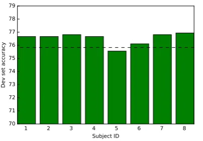
Figure 4: Accuracy on the development set for the different subjects when trained and tested on fMRI data from only this one subject. Dashed line is the development set baseline. Only in one out of eight cases does adding fMRI features lead to worse per-formance.

EM-HMM Parameters We use the same set-ting as Li et al. (2012) for the number of EM iterations, fixing this parameter to 30 for all ex-periments.

5 Experiments

Experimental setup From the neuro-imaging dataset described above, we use 41 sentences (720 tokens) as a development set and 41 sentences (529 tokens) as a test set, and the remaining 326 sentences (corresponding to 80%) for training our model.

Basic features The basic features of all the mod-els (except when explicitly stated otherwise) are based on seven features that we adopt from Li et al. (2012), capturing word form, hyphenation, suf-fix patterns, capitalization and digits in the token.

Wiktionary Of the 1,411 word types in the cor-pus, we find that 1,381 (97.84%) are covered by the Wiktionary dump made available by Li et al. (2012),1 _{which we use as our type constraints} when inducing our models.

5.1 Part-of-speech annotation

Though Wehbe et al. (2014) also provide syntac-tic information, these are automasyntac-tic parses that are not suitable for the evaluation of our model. The development and test data are therefore manually

1_{https://code.google.com/archive/p/} wikily-supervised-pos-tagger/

annotated for universal part-of-speech tags (Petrov et al., 2011) by two linguistically trained annota-tors. The development set was annotated by both annotators, who reached an inter-annotator agree-ment of 0.926 in accuracy and 0.928 in weighted F1. For the final development and test data,

dis-agreements were resolved by the annotators.

5.2 Non-fMRI baselines

Our first baseline is a second-order HMM with type constraints from Wiktionary; this in all re-spects the model proposed by Liu et al. (2012), ex-cept trained on our small Harry Potter corpus. In a second baseline model, we also incorporate 300-dimensional GloVe word embeddings trained on Wikipedia and the Gigaword corpus (Pennington et al., 2014). We also test a version of the baseline without the basic features to get an estimate of the contribution of this aspect of the setup.

5.3 Token-level fMRI

We run a series of experiments with token-level fMRI vectors that we obtain as described in Sec-tion 3.2.1. Initially, we train separate models for each of the eight individual subjects, whose per-formance on the development data are illustrated in Figure 4.

5.3.1 Tuning hyperparameters

We tune the following hyperparameters on the token-level development set in the following or-der: the number of subjects to use, the number of principal components per subject, and the time window. For the earlier tuning processes we fix the later hyperparameters to values we consider rea-sonable, but once we have tuned a hyperparameter, we use the best value from this tuning process for later tuning steps. The initial values are: 10 prin-cipal components and a time window of [t+ 0s, t+ 6s].

1 2 3 4 5 6 7 8 Number of subjects

75.0 75.5 76.0 76.5 77.0 77.5

Dev set accuracy

(a) Learning curve for increasing number of subjects in the model. Fixed hyper-parameters: 10 principal components and a time window of [t+ 0s,t+ 6s].

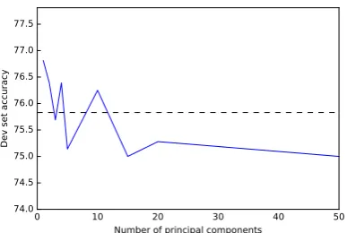
0 10 20 30 40 50

Number of principal components 74.0

74.5 75.0 75.5 76.0 76.5 77.0 77.5

Dev set accuracy

(b) Learning curve for increasing number of principal com-ponents per subject in the model. Number of principal components ∈ {1,2,3,4,5,10,15,20,50} Fixed hyper-parameters: 8 subjects, a time window of [t+ 0s,t+ 6s]. Figure 5: Exploring two individual hyper-parameters of the model on development set. Dashed lines indicate the development set baseline.

the eigenvectors that we obtain for different sub-jects, such that the feature vectors grow in length as the number of included subjects increases.

As Figure 5a shows, exploring an increasing number of subjects in the model does not seem to a have consistent effect on development set accu-racy. However, we expect an increased robustness from a model that incorporates a greater number of subjects. In all following experiments we there-fore use data from all eight readers, but we would also expect a model with fewer subjects to perform reasonably.

Principal components Fixing the number of subjects to eight, we then perform experiments to determine the number of principal components per subject to consider in our model, whose results are visualized in Figure 5b. We observe the first eigen-vectors carry a strong signal, while a great number of principal components tends to water down the signal and lead to worse performance. We choose to continue using 10 dimensions in all further ex-periments.

Time window for token vectors We next run experiments to determine the optimal time win-dow for the computation of the token vectors, us-ing different combinations of start and end times in relation to the token time stamps, but keeping the number of subjects and principal components constant at eight and ten, respectively. These ex-periments yield three different time windows with an equally good performance on the development set: [t−4s,t+ 10s], [t+ 2s,t+ 8s] and [t+ 0s,

t+ 6s]. Note that due to the Gaussian weighting the centre of the interval gets more weight than the edges and that [t−4s,t+10s] and [t+0s,t+6s] have the same centre,t+ 3. While [t+ 2s,t+ 8s] and [t+0,t+6] align better with psycholinguistic expectations, [t−4s, t+ 10s] makes our model less prone to overfitting. We therefore select the model averaging over the largest time window.

5.4 Type-level fMRI aggregates

Next, we aggregate token vectors to compute their type-level averages, in an effort to explore to which degree neural activity is dependent on the read word type rather than the concrete grammat-ical environment, and whether this can allow our model to draw conclusions about the grammatical class of a token. We compute the type-level aggre-gates as the component-wise arithmetic mean of the token vectors that we extract using the param-eter settings optimized above. Note, however, that out of the 4,898 tokens in the text, 823 (16.9%) occur only once.

6 Results

Table 1 reports the results that we obtain with our final hyper-parameter settings, which are as fol-lows:

Number of subjects 8 Principal components 10 Start of time window t−4s End of time window t+ 10s

consid-Accuracy Baseline (Li et al., 2012) 69.57

Baseline+GloVe 69.38

Baseline w/o basic feats 55.53 fMRI (token-level) w/o basic feats 56.99

fMRI (type-level) 70.32

fMRI (token-level) 70.89

Error reduction over baseline 04.34

Table 1: Tagging accuracy on test data for the dif-ferent models. The fMRI model is significantly better than the baseline (p= 0.014, Bootstrap).

Class Prec. Rec. F1 ±BL ADJ 37.50 42.86 40.00 +2.71 ADP 83.67 77.36 80.39 +1.54 ADV 66.00 58.93 62.26 +5.69 CONJ 70.97 70.97 70.97 ±0.00 DET 80.49 80.49 80.49 +3.38 NOUN 70.37 76.00 73.08 +0.28 NUM 00.00 00.00 00.00 -20.00 PRON 88.68 74.60 81.03 +4.76 PRT 41.67 41.67 41.67 +11.67 VERB 74.36 76.32 75.32 -0.95

Table 2: Test data tagging performance by part-of-speech class for the best fMRI model. The right-most column displays the difference in F1

com-pared to the baseline model.

erable error reduction over the baseline model as well as the embeddings-enriched baseline model. It also outperforms the model which uses type-level averages over the fMRI recordings. Leaving out the basic features hurts performance, but even without the basic features the fMRI data can re-duce error with 3.28% on the test set. In Table 2 we present the performance on the individual PoS classes under our best model.

7 Analysis and Discussion

7.1 What’s in the fMRI vectors?

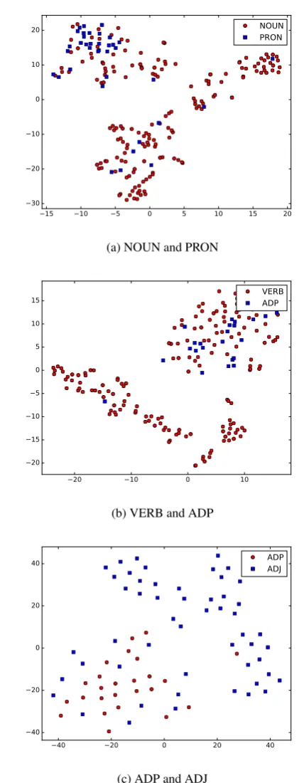
t-SNE (Van der Maaten and Hinton, 2008) is a powerful supervised dimensionality reduction tool for visualizing high-dimensional data in two-dimensional space using Stochastic Neighbor Em-bedding. In Figure 6, we visualize pairs of PoS classes of the test data in a two-dimensional

re-15 10 5 0 5 10 15 20

30 20 10 0 10

20 NOUN

PRON

(a) NOUN and PRON

20 10 0 10

20 15 10 5 0 5 10

15 VERB_ADP

(b) VERB and ADP

40 20 0 20 40

40 20 0 20

40 ADP_ADJ

(c) ADP and ADJ

duction of the embedding space obtained when us-ing the settus-ings of the best fMRI model. The fact that we can discriminate reasonably well between, e.g., nouns and pronouns, verbs and adpositions, as well as adpositions and adjectives on the basis of fMRI data is to the best of our knowledge a new finding.

7.2 Discussion of the results

We showed that by careful model tuning and de-sign it is possible to extract a de-signal of grammati-cal processing in the brain from fMRI. The figures that we present in Table 1 reflect, to our knowl-edge, the first successful results in inferring gram-matical function at the token level from fMRI data. Our best model, which we train on the ten princi-pal components from the fMRI recordings of eight readers, achieves an error reduction of over 4% de-spite a very small amount of training data. We find that our best model uses a very wide window of fMRI recordings to compute the representations for individual tokens, considering all recordings from 4 seconds before the token is displayed until 10 seconds after the token is displayed. Our best explanation for why the incorporation of preced-ing fMRI measurements is beneficial to our model, is that the grammatical function of a token may be predictable from a reader’s cognitive state while reading preceding tokens. However, note that the measurements at the far ends of the time window only factor into the token vector to a small degree as a consequence of the Gaussian weighting. Our experiments further suggest that using token-level information instead of type-level features, such as word embeddings or type averages of fMRI vec-tors, is helpful for PoS induction that already is type-constrained.

Recently, Huth et al. (2016) found that semanti-cally related words are processed in the same area of the brain. Open questions for future work in-clude whether there is a bigger potential for using fMRI data for semantic rather than syntactic NLP tasks, and whether the signal we find mainly stems from semantic processing differences.

8 Conclusion

This paper presents the first experiments induc-ing part of speech from fMRI readinduc-ing data. Cog-nitive psychologists have debated whether gram-matical differences lead to different brain activa-tion patterns. Somewhat surprisingly, we find that

1 5 10 15 20 25 30

Number of iterations 68

69 70 71 72 73 74 75 76 77

Dev. tagging accuracy

full baseline

Figure 7: Learning curve of tagging accuracy on the development set as a function of different num-ber of EM iterations for baseline model and the full model for iteration numbers∈ [1,30]. Fixed hyper-parameters: 8 subjects, 10 principal compo-nents, and a time window oft−4stot+ 10s

the fMRI data contains a strong signal, enabling a 4% error reduction over a state-of-the-art unsu-pervised PoS tagger. While our approach may not be readily applicable for developing NLP models today, we believe that the presented results may inspire NLP researchers to consider learning mod-els from combinations of linguistic resources and auxiliary, behavioral data that reflects human cog-nition.

Acknowledgements

This research was partially funded by the ERC Starting Grant LOWLANDS No. 313695, as well as by Trygfonden.

Supplementary material

Number of EM iterations As supplementary material, we present the EM learning curve in Fig-ure 7, which shows a steep learning curve at the beginning and relatively stable performance fig-ures after 15 iterations for the full model and 10 iterations for the baseline model.

References

Maria Barrett, Joachim Bingel, Frank Keller, and An-ders Søgaard. 2016. Weakly supervised part-of-speech induction using eye-tracking data. InACL. Taylor Berg-Kirkpatrick, Alexandre Bouchard-Cote,

John DeNero, and Dan Klein. 2010. Painless un-supervised learning with features. InProceedings of

Manuela Berlingeri, Davide Crepaldi, Rossella Roberti, Giuseppe Scialfa, Claudio Luzzatti, and Eraldo Paulesu. 2008. Nouns and verbs in the brain: Grammatical class and task specific effects as revealed by fMRI. Cognitive Neuropsychology, 25(4):528–558.

Ron Borowsky, Carrie Esopenko, Layla Gould, Naila Kuhlmann, Gordon Sarty, and Jacqueline Cummine. 2013. Localisation of function for noun and verb reading: converging evidence for shared processing from fmri activation and reaction time. Language and Cognitive Processes, 28(6):789–809.

V´eronique Boulenger, Alice C Roy, Yves Paulignan, Viviane Deprez, Marc Jeannerod, and Tatjana A Nazir. 2006. Cross-talk between language pro-cesses and overt motor behavior in the first 200 msec of processing. Journal of cognitive neuroscience, 18(10):1607–1615.

Julio Gonz´alez, Alfonso Barros-Loscertales, Friede-mann Pulverm¨uller, Vanessa Meseguer, Ana Sanju´an, Vicente Belloch, and C´esar ´Avila. 2006. Reading cinnamon activates olfactory brain regions.

Neuroimage, 32(2):906–912.

Daniel A Handwerker, Javier Gonzalez-Castillo, Mark D’Esposito, and Peter A Bandettini. 2012. The continuing challenge of understanding and model-ing hemodynamic variation in fmri. Neuroimage, 62(2):1017–1023.

Alexander G Huth, Wendy A de Heer, Thomas L Grif-fiths, Fr´ed´eric E Theunissen, and Jack L Gallant. 2016. Natural speech reveals the semantic maps that tile human cerebral cortex. Nature, 532(7600):453– 458.

Sigrid Klerke, Yoav Goldberg, and Anders Søgaard. 2016. Improving sentence compression by learning to predict gaze. InNAACL.

Shen Li, Jo˜ao Grac¸a, and Ben Taskar. 2012. Wiki-ly supervised part-of-speech tagging. In EMNLP, pages 1389–1398.

Dong C Liu and Jorge Nocedal. 1989. On the limited memory bfgs method for large scale optimization.

Mathematical programming, 45(1-3):503–528.

Xiaohua Liu, Ming Zhou, Furu Wei, Zhongyang Fu, and Xiangyang Zhou. 2012. Joint inference of named entity recognition and normalization. In

ACL, pages 526–535.

Rachel L Moseley and Friedemann Pulverm¨uller. 2014. Nouns, verbs, objects, actions, and abstrac-tions: local fmri activity indexes semantics, not lex-ical categories. Brain and language, 132:28–42. Seiji Ogawa, David W Tank, Ravi Menon, Jutta M

Ellermann, Seong G Kim, Helmut Merkle, and Kamil Ugurbil. 1992. Intrinsic signal changes ac-companying sensory stimulation: functional brain

mapping with magnetic resonance imaging.

Pro-ceedings of the National Academy of Sciences,

89(13):5951–5955.

Jeffrey Pennington, Richard Socher, and Christopher D Manning. 2014. Glove: Global vectors for word representation. InEMNLP, volume 14, pages 1532– 1543.

Slav Petrov, Dipanjan Das, and Ryan McDonald. 2011. A universal part-of-speech tagset. CoRR abs/1104.2086.

Cathy J Price. 2012. A review and synthesis of the first 20years of pet and fmri studies of heard speech, spo-ken language and reading. Neuroimage, 62(2):816– 847.

M-A Tagamets, Jared M Novick, Maria L Chalmers, and Rhonda B Friedman. 2000. A parametric ap-proach to orthographic processing in the brain: an fmri study. Cognitive Neuroscience, Journal of, 12(2):281–297.

Scott Thede and Mary Harper. 1999. A second-order hidden markov model for part-of-speech tagging. In

ACL, pages 175–182.

Lorraine Tyler, Peter Bright, Paul Fletcher, and Em-manuel Stamatakis. 2004. Neural processing of nouns and verbs: The role of inflectional

morphol-ogy. Neuropsychologia, 42(4):512–523.

Laurens Van der Maaten and Geoffrey Hinton. 2008. Visualizing data using t-sne. Journal of Machine

Learning Research, 9(2579-2605):85.