Emission Cap Commitment versus Emission Intensity Commitment as Self Regulation

Munich Personal RePEc Archive

Emission Cap Commitment versus

Emission Intensity Commitment as

Self-Regulation

Hirose, Kosuke and Matsumura, Toshihiro

10 November 2017

Online at

https://mpra.ub.uni-muenchen.de/82564/

Emission Cap Commitment versus Emission Intensity

Commitment as Self-Regulation

Kosuke Hirose

_{and Toshihiro Matsumura}

November 10, 2017

Abstract

We compare emission cap commitment that restricts total emissions and emis-sion intensity commitment that restricts emisemis-sions per unit of output as measures of self-regulation. The monopolist chooses either emission cap commitment or emis-sion intensity commitment and sets the target level under the constraint that the resulting emissions do not exceed the upper limit. We find that profit-maximizing firms choose emission cap commitment, although emission intensity commitment al-ways yields greater consumer surplus. It is ambiguous whether emission intensity commitment or emission cap commitment yields greater welfare. We present two cases in which emission intensity commitment yields greater welfare. One is the most stringent target case (the target emission level is close to zero), and the other is the weakest target case (the target emission level is close to business-as-usual). Our re-sult suggests that the incentive for adopting emission cap commitment is too large for profit-maximizing firms, and thus, governments should encourage the adoption of emission intensity commitment, especially to achieve a zero-emission society efficiently.

JEL classification codes: Q52, L12, L51

Keywords: self-regulation, emission intensity, emission cap, monopoly, zero-emission

∗_{This work was supported by JSPS KAKENHI (15K03347,16J04589) and Zengin Foundation for Studies}

on Economics and Finance.

†_{Corresponding author, Graduate School of Economics, The University of Tokyo, 7-3-1, Hongo,}

Bunkyo-ku, Tokyo, 113-0033, Japan. E-mail:[email protected]

‡_{Institute of Social Science, The University of Tokyo, 7-3-1, Hongo, Bunkyo-ku, Tokyo, 113-0033, Japan.}

1

Introduction

Self-regulatory actions by an industry or firms have received considerable attention from

economists and policymakers. In particular, self-regulation has been introduced in

environ-mental policies as a tool to improve the environment, in addition to command-and-control

regulation and/or economic incentives, such as emission taxes and tradable permits. Firms

publicly initiate pledges to improve their environmental performance and undertake efforts

to attain the goals by themselves.1

A typical question regarding self-regulation is why firms

voluntarily take certain actions even though they are costly. The literature on self-regulation

suggests that polluting firms strategically act and self-regulate because of the threat of

fu-ture regulation by regulatory authorities (e.g., Maxwell et al., 2000; Antweiler, 2003; Lyon

and Maxwell, 2003; Fleckinger and Glachant 2011). Maxwell et al. (2000) formulated a

theoretical model in which firms can choose their levels of voluntary pollution prior to

po-litical action by consumers leading to mandatory regulation and showed that self-regulation

effectively preempts political entry. Antweiler (2003) empirically tested the effect of green

regulatory threat. In addition, private politics, such as a boycott, have been used to explain

the motivation of voluntary actions. Egorov and Harstad (2017) examined the interaction

among public regulation, self-regulation, and boycott as private politics and showed the

possibility of self-regulation. There is, however, another natural question to self-regulation:

what measure should firms adopt as self-regulation?

There are several ways to commit to improve environmental performance.2

Consider

air pollution or carbon dioxide (CO2) emissions. A commitment to decrease the total

1

This form of self-regulation is called “unilateral commitments” in which the target is set by the industry or companies themselves. The OECD (1999) categorized voluntary environmental agreements into the three categories of unilateral commitments, public voluntary programs, and negotiated agreements.

2

emissions or to limit the upper bound of emissions per year is a direct measure (emission

cap commitment). On the other hand, the emission intensity per unit of output is another

popular measure (emission intensity commitment).3

The choice of commitment device might

affect the behavior of firms and resulting welfare.4

We formulate a self-regulation model in which the polluting firm self-regulates to

pre-empt mandatory regulation or to avoid consumer activism, and then the firm determines its

output and abatement. The model employs a general formulation of a monopoly setting to

highlight the difference between emission intensity commitment and emission cap

commit-ment as measures of self-regulation. Our central concerns are which of emission intensity

commitment or emission cap commitment is chosen by the pollutant, and the ranking of

consumer surplus and social welfare between these two measures of self-regulation. We

compare the equilibrium outcomes at the environmental target, which is a common

require-ment regardless of the measure of self-regulation. Specifically, the environrequire-mental target is

assumed the total amount of emissions.

We find that the equilibrium abatement investment and output are larger (and thus,

consumer surplus is larger) under emission intensity commitment than under emission cap

commitment. By contrast, emission cap commitment yields higher profit than does emission

intensity commitment. Therefore, profit-maximizing firms choose emission cap commitment

as a self-regulation tool. From a welfare perspective, however, it is ambiguous whether

emis-sion cap commitment or emisemis-sion intensity commitment is better. We find that emisemis-sion

intensity commitment is unambiguously better than emission cap commitment in two

im-3

Japanese electric power companies have committed to CO2 emissions/kWh, not total emissions, as self-regulation. Japanese Ministry of the Environment has declared that it would introduce stricter regulation if this self-regulation were to turn out not to work effectively.

4

portant cases: in the case with the strictest target (when the emission target is close to

zero emissions) and in the case with the loosest target (when the emission target is close

to the business-as-usual level). Firms prefer emission cap commitment even when emission

intensity commitment is desirable for welfare. Thus, our result suggests that the incentive to

adopt emission cap commitment is too strong for profit-maximizing firms as a self-regulation

measure and governments should encourage the adoption of emission intensity commitment

rather than emission cap commitment, especially to achieve a zero-emission society

effi-ciently.

However, emission cap commitment can yield greater welfare. We show that emission

cap commitment can yield greater welfare, depending on the emission target level and the

curvature of the abatement cost function. If the target level is far from both zero emission

and business-as-usual levels, and the convexity of the abatement cost function is strong,

emission cap commitment is better for welfare.

The rest of this study is organized as follows. Section 2 describes the model. Section 3

analyzes and compares the two self-regulation measures of emission intensity commitment

and emission cap commitment. Section 4 concludes.

2

The Model

We consider the self-regulation model of a polluting monopoly.5

The firm produces a single

commodity for which the inverse demand function is given by P(q) :_R+ 7→R+. We assume

that P(q) is twice continuously differentiable and P′_{(q)<0 for all q as long as P >0. Let}

C(q) : R+ 7→R+ be the cost function of the firm, where q ∈R+ is the output of the firm.

We suppose C is twice continuously differentiable, increasing, and convex for all q.6 We

assume that the marginal revenue is decreasing (i.e., 2P′_{(q) +P}′′_{(q)q < 0). This condition}

5

Our results hold in symmetric Cournot oligopolies under the standard conditions (e.g., stability condi-tions).

6

guarantees that the second-order condition is satisfied.

Some emissions are associated with production, which yields a negative externality. After

emissions have been generated, they can be reduced by the polluting firm through investment

in abatement technologies.7

Thus, the firm’s net emissions areE :=g(q)−x, whereg :R+7→

R+ represents emissions associated with production and x(∈ R+) is the firm’s abatement

level. We assume that g is twice continuously differentiable, increasing, and convex for all

q.

The firm’s profit is

P(q)q₋C(q)₋K(x),

where the third term represents the abatement cost. We suppose that K is twice

contin-uously differentiable, increasing, and strictly convex for x > 0. We further assume that

K(0) =K′_{(0) = 0.}8

This assumption guarantees that the social optimal level of abatement

is never zero and that the profit function is smooth.

Total social surplus (firm profits plus consumer surplus minus the loss caused by the

externality) is given by

W =π+CS−η(E) =

∫ q

0

P(z)dz−C(q)−K(x)−η(E),

where η:R+7→R+ is the welfare loss of emissions.

The firm undertakes self-regulation through emission intensity commitment or emission

cap commitment. One might consider that the regulator should impose an emission tax

or mandatory regulation on the polluting firm in order to restrict emissions rather than

relying on self-regulation. The situation this study considers is similar to that of Segerson

and Miceli (1998), Lyon and Maxwell (2003), Glachant (2007), and Brau and Carraro (2011).

7

These are called end-of-pipe technologies. An alternative approach to reduce emissions is to change the production process. For a recent discussion of the relationship between mandatory regulation and this type of innovation, see Matsumura and Yamagishi (2017).

8

Self-regulation might be preferable to mandatory regulation, since the former reduces the

administrative cost associated with serious mandatory regulation by law or avoids political

resistance from regulated industry. Alternatively, if the government plans to impose an

emission tax to reduce total emissions to ¯E and firms expect the possible introduction of an

emission tax following self-regulation, the firms would introduce self-regulation that yields

E = ¯E to prevent the introduction of such an emission tax.

An alternative interpretation of the environmental target that the polluting firm

volun-tary commits to is based on consumer activism. Unlike lobbying or political campaigns,

consumers who have disutility from negative externalities organize activist groups and start

a boycott if their requirements are not met (Egorov and Harstad, 2017). In this case, it is

natural to consider that their concern is emission levels.

We assume that the environmental target is exogenously given. In other words, we

do not model the regulator and the activist group as players. As discussed earlier in this

section, we can describe ¯E depending on the administrative cost, political pressure, or the

opportunity cost of the consumer boycott. There are, however, several ways to formulate

such regimes so that we simply treat the target as an exogenous variable and examine how

the firm undertakes self-regulation at each level, ¯E. We assume that ¯E _∈(0, EB_{) whereE}B

is the profit-maximizing emission level without a binding emission target (business-as-usual

level). Let qB _{be the profit-maximizing output without a binding emission target.}

The timing of the game is as follows. Given the environmental target, ¯E, the firm

decides whether to use emission intensity commitment or emission cap commitment in the

first stage. In the second stage, the firm chooses its output and abatement level to maximize

the profit under the self-regulation it committed to in the first stage.

3

Analysis

3.1

Emission Intensity Commitment

First, we consider the case in which the firm adopts emission intensity commitment as

self-regulation. Let αbe the committed upper bound of the emission per unit of output. In the

second stage, the firm chooses its output, q, and abatement level, x, to maximize its profit

subject to

α_≥ E q =

g(q)−x

q . (1)

When the constraint is binding9

, the firm’s optimization problem is

max

q P(q)q−C(q)−K(g(q)−αq). (2)

Let the superscript EI denote the equilibrium outcomes under emission intensity

commit-ment. Define πEI_{(q;α) :=P(q)q}

−C(q)₋K(g(q)₋αq). The equilibrium output, qEI_(α),

is characterized by the following first-order condition:

∂πEI

∂q =P

′_q+P

−C′−K′(g′ −α) = 0. (3)

The second-order condition is satisfied. We obtain xEI_{(α) = g(q}EI_(α))

− αqEI_{(α) and}

EEI_{(α) = g(q}EI_(α))

−xEI_{(α) = αq}EI_(α).

Differentiating (3) leads to

dqEI

dα =− ∂2

π/∂q∂α

∂2_π/∂q2 >0, (4)

where we use ∂2

π/∂q∂α =K′_{+ (g}′

−α)K′′_{q >0 and ∂}2

π/∂q2

= 2P′_+P′′_q

−C′′

−g′′_K′

−

(g′_−α)2

K′′ _{<0. An increase in αrelaxes the emission restriction and reduces the marginal}

cost of production, which increases q.

In the first stage, the firm sets the emission intensity α = ¯α such that EEI_{(¯α) = ¯E.}

Let (qEI_{( ¯E), x}EI_{( ¯E)) be the pair of equilibrium output and abatement and W}EI_{( ¯E) be the}

equilibrium welfare under emission intensity commitment whenα = ¯α.

9

3.2

Emission Cap Commitment

Next, we consider the case in which the firm adopts emission cap commitment. The profit

function of the firm is P(q)q −C(q)−K(g(q)−E¯). Let the superscript EC denote the

equilibrium outcomes under emission cap commitment. Then, the profit function of the firm

under emission cap commitment is defined by πEC_{(q; ¯E) := P(q)q}

−C(q)−K(g(q)−E¯).

The equilibrium output, qEC_{( ¯E), is characterized by the following first-order condition:}

∂πEC

∂q =P

′_q+P

−C′₋K′g′ = 0. (5)

The second-order condition is satisfied. We obtainxEC_{( ¯E) = g(q}EC_{( ¯E))}

−E¯. Differentiating

(5) leads to

dqEC

dE¯ =− ∂2

π/∂q∂E¯

∂2_π/∂q2 >0, (6) where we use ∂2

π/∂q∂ = K′′_g′ _{> 0 and ∂}2

π/∂q2

= 2P′_+P′′_q

−C′′

−g′′_K′

−g′2

K′′ _{< 0.}

Similar to the emission intensity case, an increase in ¯E increasesq.

3.3

Comparison

In this subsection, we compare the two instruments. First, we consider the equilibrium

output. Comparing emission intensity commitment with emission cap commitment, we

present the following result.

Lemma 1The equilibrium output is larger under emission intensity commitment than under

emission cap commitment, that is, qEI_{( ¯E)> q}EC_{( ¯E).}

Proof.

By using (3), (5), and the emission equivalence, we obtain

∂πEC

∂q

q=qEI = K

′_(g(qEI

)−αq¯ EI)[

(g′(qEI)−α¯]

−K′(g(qEI)−E¯)g′(qEI)

= −K′(g(qEI)−αq¯ EI)¯α <0.

This implies that the output level of qEI _{exceeds the profit-maximizing level under emission}

Lemma 1 states that the firm produces more outputs under emission intensity

commit-ment than under emission cap commitcommit-ment even though the resulting emissions from the

pollutant are the same in both regimes. We explain the intuition behind Lemma 1 after

presenting Proposition 1.

From Lemma 1 and the emission equivalence, we obtain the following lemma.

Lemma 2 Emission intensity commitment yields greater net consumer surplus than

emis-sion cap commitment, that is, CS(qEI_{( ¯E)}

−η( ¯E)> CS(qEC_{( ¯E))}

−η( ¯E).

Proof.

It is straightforward from the emission equivalence and Lemma 1. ■

We now present our result on the firm’s profit.

Proposition 1 Emission cap commitment yields higher profit than does emission intensity

commitment (i.e., πEC_(qEC_{( ¯E),E}¯_{)> π}EI_(qEI_{( ¯E),α¯).}

Proof.

Using the resulting profit and the emission equivalence, we obtain

πEC(qEC,E¯) = P(qEC)qEC−C(qEC)−K(g(qEC)−E¯)

> P(qEI)qEI −C(qEI)−K(g(qEI)−E¯)

= P(qEI_)qEI

−C(qEI₎

−K(g(qEI₎

−αq¯ EI_{) = π}EI_(qEI_,α¯),

where the inequality follows from the fact that arg max{q}P(q)q−C(q)−K(g(q)−E¯) =qEC

and qEI

̸

=qEC_.

■

We explain the intuition behind Lemma 1 and Proposition 1. Under emission intensity,

the firm faces a time-inconsistency problem. In the second stage, given α, an increase in q

increases the upper limit of emissions. Therefore, the firm has a stronger incentive to increase

its output than under emission cap commitment (Lemma 1). However, this makes it stricter

profit. Therefore, the firm’s profit is larger under emission cap commitment, which does not

yield such a time-inconsistency problem, than under emission intensity commitment.

We now discuss social welfare. Emission intensity commitment is superior for consumer

welfare than is emission cap commitment (Lemma 2), but is less profitable for the firm

(Proposition 1). Thus, it is generally ambiguous which is socially preferable. Let WEI_{( ¯E)}

andWEC_{( ¯E) be the equilibrium welfare under emission intensity commitment and emission}

cap commitment, respectively. We present two cases in which emission intensity

commit-ment yields greater welfare than emission cap commitcommit-ment (i.e., WEI_{( ¯E) > W}EC_{( ¯E)).}

First, we consider the case with the most stringent target case ( ¯E is close to zero). When

the firm is not allowed to pollute in the process of producing output (i.e., ¯E = ¯α = 0), all

emissions are reduced by the abatement activities and there are no emissions in the

indus-try. Regardless of the output level, the total emissions are zero if and only if emissions per

unit of output are zero. Therefore, when ¯E = 0, emission cap commitment and emission

intensity commitment yield the same outcome. Let qZ _{and x}Z _{be common q and x under}

the zero-emission constraint (i.e., when ¯E = 0).

We now present a result when ¯E is close to zero.

Proposition 2 If E¯ is sufficiently close to zero, emission intensity commitment yields

greater welfare than does emission cap commitment.

Proof.

Fori=EC, EI, we obtain

∂Wi

∂E¯

_E¯₌₀ =

∂W ∂q

dqi

dE¯ + ∂Wi

∂x dxi

dE¯ + ∂Wi

∂E

= (P(qZ)−C′(qZ))dq i

dE¯ −K

′_(xZ )dx

i

dE¯ −η

′₍₀₎

= (P(qZ)−C′(qZ))dq i

dE¯ −K

′_(xZ )

(

g′(qZ)dq i

dE¯ −1

)

−η′(0)

= (P(qZ₎

−C′(qZ₎

−K′(xZ_)g′_(qZ₎₎dqi

dE¯ +K

′_(xZ₎

where we useg−x= ¯E(and thus,dxi_/dE¯ _=g′_(dqi_/dE¯₎

−1), and (qEC_{, x}EC_{) = (q}EI_{, x}EI_{) =}

(qZ_{, x}Z_{) when ¯E = 0. Because q}Z _{< q}EC _{< q}EI _{for all ¯E >0, we obtain}

dqEI

dE¯

_E¯₌₀>

dqEC

dE¯

_E¯₌₀.

From (5), we obtain P −C′−K′g′ > P +P′q−C′−K′g′ = 0. Under these conditions, we

obtain

∂WEI

∂E¯

_E¯₌₀>

∂WEC

∂E¯

_E¯₌₀. Because WEI _=WEC _{when ¯E = 0, we obtain Proposition 2. ■}

The intuition behind the result is as follows. As we explained after Proposition 1, given

¯

α > 0, the firm has a stronger incentive to expand its output under emission intensity

commitment than under emission cap commitment, because under emission intensity, the

firm can increase the upper limit of emissions in the second stage (time-inconsistency

prob-lem). However, this problem does not exist when ¯E = ¯α = 0. Therefore, qEC _{= q}EI _and

xEC _=xEI _{when ¯E = ¯α= 0.}

An increase in ¯α relaxes the restriction on emissions. This leads to an increase in

emissions, resulting in larger disutility from the emissions (emission effect). However, by

the assumption of emission equivalence between two regimes, the emission effect is the same

for two regimes. An increase in ¯E and ¯αaffects qandx(allocation effect). As stated above,

emission intensity commitment yields larger q and x than emission cap commitment does.

Given the emission level, under emission cap commitment, the marginal social cost of

the reduction of emissions by reduction of q is P/g′ _{and that by the increase of x is K}′_.

The marginal private cost for meeting the constraint by the reduction of q for the firm is

(P+P′_q)/g′ _{and that by the increase ofx isK}′_{. Thus, both xandq chosen by the firm are}

too small for social welfare. Given the emission level, under emission intensity, the marginal

private cost for meeting the constraint by the reduction ofqfor the firm is (P+P′_q)/(g′_−α)

still too small for social welfare, but both are larger than under emission cap commitment.

Therefore, emission intensity commitment is better for social welfare than is emission cap

commitment.

We believe that the most stringent case discussed in Proposition 2 is important. Under

the Paris Climate Agreement, many countries, such as the UK, France, Germany, and Japan,

plan to reduce CO2 emissions drastically by 2050 (about 80% reduction at least against a

business-as-usual scenario). To achieve this goal, several industries, such as electric power

and transport, an emission constraint that is close to zero emissions might be imposed.

Thus, the most stringent case discussed in Proposition 2 might be realistic.

Next, we examine the opposite case, the loosest constraint case in which ¯E is close to

EB_.

Proposition 3Suppose that E¯ is sufficiently close to EB_{. Emission intensity commitment}

yields greater welfare than does emission cap commitment.

Proof.

Fori=EC, EI, we obtain

∂Wi

∂E¯

_E¯_=EB =

∂W ∂q

dqi

dE¯ + ∂Wi

∂x dxi

dE¯ + ∂Wi

∂E

= (P(qB₎

−C′(qB₎₎dqi

dE¯ −K

′_(xB₎dxi

dE¯ −η

′_{( ¯E)}

= (P(qB)−C′(qB))dq i

dE¯ −η

′_,

where we use qEC _=qEI _=qB _{and x}EC _=xEI _{= 0 when ¯E =E}B _{and K}′_{(0) = 0. Because}

qEC _{< q}EI _{< q}B _{for all ¯E < E}B_{, we obtain}

dqEI

dE¯

_E¯_=EB>

dqEC

dE¯

_E¯_=EB.

From (5), we obtain P ₋C′ _{>0. Under these conditions,}

∂WEI

∂E¯

_E¯_=EB>

∂WEC

∂E¯

Because WEI _=WEC _{when ¯E =E}B_{, we obtain Proposition 3.}

■

We explain the intuition behind Proposition 3. Because of emission equivalence, the

emission effect is the same between two regimes. When ¯E = EB_{, q}EC _{= q}EI _{= q}B _and

xEC _=xEI _{= 0. Because K}′_{(0) = 0, this abatement level is too low for social welfare, and}

a marginal reduction of emissions by an increase in x is much more efficient than that by

a reduction in q for social welfare. In other words, given the emission, q is too large and x

is too small for social welfare. A marginal decrease in ¯α increases x and reduces q under

both emission cap commitment and emission intensity commitment, which improves welfare.

The magnitude of this effect is stronger under emission intensity commitment. Note that

qEI _{> q}EC _{and thus, x}EI _{> x}EC _{for ¯E}

∈(0, EB_).

In Propositions 2 and 3, we show that when the target level is close to the strictest

and loosest cases, emission intensity commitment is better for social welfare than emission

cap commitment. Emission intensity commitment stimulates production and mitigates the

problem of suboptimal production and abatement investment, which improves welfare under

emission equivalence. Because emission intensity commitment is better for social welfare

in the two polar cases, it might be natural to guess that emission intensity commitment is

better for any ¯E _∈(0, EB_{). However, this is not true.}

Let (

x∗_{( ¯E), q}∗_{( ¯E)})

be the pair of the second–best abatement and output level (social

optimumx and q givenE = ¯E). The derivation is as follows. Given ¯E, the social planner’s

problem is

max

q,x W =

∫ q

0

P(z)dz−C(q)−K(x)−η( ¯E)

s.t. E¯ =g(q)−x.

The second-best output level, q∗_{( ¯E), is characterized by the following first-order condition:}

∂W

∂q =P −C

′

x∗( ¯E) is derived from ¯E =g(q∗)−x∗.

As discussed above, qEC_{( ¯E) < q}∗_{( ¯E) and thus, x}EC_{( ¯E) < x}∗_{( ¯E). Note that q}EC_{( ¯E) is}

derived P +P′_q

−C′

−K′_g′ _{= 0. In the two polar cases (the strictest and loosest cases),}

(

xEC_{( ¯E), q}EC_{( ¯E)})

=(

xEI_{( ¯E), q}EI_{( ¯E)})

.Except for the two polar cases,(

xEC_{( ¯E), q}EC_{( ¯E)})

<

(

xEI_{( ¯E), q}EI_{( ¯E)})

holds. As long as(

xEC_{( ¯E), q}EC_{( ¯E)})

<(

xEI_{( ¯E), q}EI_{( ¯E)})

<(

x∗_{( ¯E), q}∗_{( ¯E)})

,

the outcome under emission intensity commitment is closer to the second-best outcome than

that under emission cap commitment, and thus, emission intensity commitment naturally

yields greater welfare than emission intensity commitment. However, it is possible that

(

xEI_{( ¯E), q}EI_{( ¯E)})

>(

x∗_{( ¯E), q}∗_{( ¯E)})

. Because emission intensity can yield excessive

produc-tion and excessive abatement investment, emission cap commitment might be better than

emission intensity commitment for social welfare.

We present an example showing that emission cap commitment could be better than

emission intensity commitment for welfare. Suppose that the inverse demand is linear

(P =a−bq), the marginal production cost is constant (normalized to zero), emissions are

proportional to output (g =eq), and the abatement cost is quadratic (K =kx2

/2). In this

example, EB _{=ae/2b and ¯α=e when ¯E =E}B_.

Straightforward calculation yields the resulting welfare for each regime. ComparingWEI

with WEC_{, we obtain the following result.}

Proposition 4 Suppose that P =a₋bq, C= 0, g =eq, and K =kx2

/2. Then,

WEI _>(<)WEC _{if k < (>)˜k,}

where

˜

k := b(2e 2

−3eα¯+ 3¯α2

+√4e4_{+ 4e}3_{α¯+ 5e}2_α¯2

−18eα¯3_{+ 9¯α}4₎ 2e2_α¯(e

−α¯) ,

lim_E¯_→0k˜= lim_E¯_→EB˜k=∞, k˜ is U-shaped with respect toE¯, and k˜≥k:= (5b+b √

89)/2e2

for any E¯ ∈(0, EB_).

Figure 1 shows this result graphically (the case in which a= 5, b = 1, and e= 2).

Emission Cap

Emission Intensity

0 1 2 3 4 EB

E

1 3

k

5

k

Figure 1: Welfare Comparison:

If k is not large, emission intensity commitment yields greater welfare regardless of ¯E.

However, if k is large, emission cap commitment yields greater welfare, because x can be

excessive under emission intensity commitment.

As discussed above, production and abatement can be excessive under emission intensity

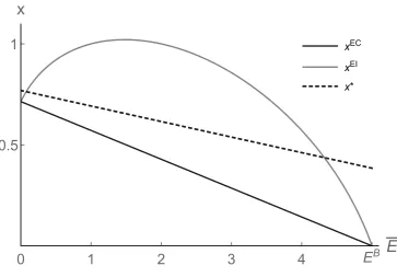
commitment, leading to Proposition 4. Figure 2 shows that x∗ _{can be smaller than x}EI_,

although x∗ _{is larger than x}EI _{regardless of ¯E (the case in which a = 5, b = 1, k = 3, and}

e = 2). In other words, the abatement level under emission intensity commitment is too

xEC

xEI

x*

0

1

2

3

4

_E

E

0.5

1

x

Figure 2: Abatement Level Comparison

4

Concluding Remarks

In this study, we compare two self-regulation tools, emission cap commitment and

emis-sion intensity commitment. We find that profit-maximizing firms always choose emisemis-sion

cap commitment. However, emission intensity commitment always yields greater consumer

welfare and can yield greater welfare. Moreover, we present two cases in which emission

intensity commitment yields greater welfare than emission cap commitment does: the case

of the strictest target, which is close to a zero-emission target, and the case of the

loos-est target, which is close to business as usual. Our result suggloos-ests that the government

should encourage the adoption of emission intensity commitment, especially to achieve a

zero-emission society efficiently, because firms prefer emission cap commitment to emission

intensity commitment, even when it is not desirable for welfare.

self-regulation before knowing the demand parameter, an increase of the degree of demand

uncertainty increases the advantage of emission intensity commitment over emission cap

commitment for both the welfare and profits of the firms. This is because the firms can

expand (shrink) their output more flexibly under emission intensity commitment than under

emission cap commitment when demand is high (low). We consider this is the reason that

some companies, such as Japanese electric power companies, choose emission intensity

com-mitments as their favored form of self-regulation. Comparing the two tools after introducing

A

Proof of Proposition 4

First, we consider the equilibrium outputs for each regime. From (3) and (5), we obtain

qEI ₌ a

2b+k(e₋α), q

EC ₌ a+keE¯ 2b+e2_k.

Substituting the equilibrium outputs into total surplus, we obtain

WEI(¯α) = a(a(3b+k(e−α¯) 2

)₋2¯αη(2b+k(e₋α¯)2 )) 2(2b+k(e−α¯)2₎2 ,

WEC_{( ¯E) =} (a 2

+ 2akeE¯)(3b+ke2

)₋E¯(bkE¯(4b+ke2

) + 2η(2b+ke2 )2

) 2(2b+ke2₎2 .

Using EEI_{(¯α) = ¯αq}EI _{= ¯E,W}EC_{( ¯E) can be rewritten as a function of ¯α. Thus, we obtain}

WEI(¯α)−WEC( ¯E) = a 2

kα¯(e−α¯)H

2(2b+k(e₋α¯)2₎2_(2b+ke2₎2

whereH := 4b2

−k2

e2 ¯

α(e₋α¯) +bk(2e2

−3eα¯+ 3¯α2

). WEI_(¯α)

−WEC_{( ¯E) is positive if and}

only if H >0 and

H >(<)0 ifk <(>)˜k= b(2e 2

−3eα¯+ 3¯α2

+√4e4 _{+ 4e}3_{α¯+ 5e}2_α¯2

−18eα¯3 _{+ 9¯α}4₎ 2e2_α¯(e

−α¯) .

Remember that ¯αis determined byEEI_{(¯α) = ¯E, thus, ˜k also depends on the emission target}

via ¯α. It implies that WEI_(¯α)>(<)WEC_{( ¯E) if k <(>)˜k. Because lim¯}

α→0˜k = lim¯α→e˜k =

∞, we obtain lim_E¯_→0k˜= lim_E¯_→EB˜k =∞.

Differentiating ˜k with ¯α, we obtain

∂˜k ∂α¯ =

b(e₋2¯α)(2e2

+eα¯₋α¯2

+√4e4_{+ 4e}3_{α¯+ 5e}2_α¯2

−18eα¯3_{+ 9¯α}4₎ ¯

α2_(e

−α¯)2√_4e4_{+ 4e}3_{α¯+ 5e}2_α¯2

−18eα¯3_{+ 9¯α}4 .

Because∂k/∂˜ α¯is negative (positive) when ¯α < (>)e/2, ˜k( ¯E) is U-shaped and is minimized

at ¯α =e/2. Because ˜k is minimized when ¯α =e/2, we obtain k = (5b+b√89)/2e2

. Note

that ¯α( ¯E) is increasing, ¯α(0) = 0,and ¯α(EB_{) =e.}

References

Amir, R., Gama, A., and Werner K. (2017). ‘On environmental regulation of oligopoly markets: emission versus performance standards’, Environmental and Resource Eco-nomics. https://doi.org/10.1007/s10640-017-0114-y

Antweiler, W. (2003). ‘How effective is green regulatory threat?’, American Economic Review, vol. 93(2), pp. 436–441.

Besanko, D. (1987). ‘Performance versus design standards in the regulation of pollution’,

Journal of Public Economics, vol. 34(1), pp. 19–44.

Brau, R. and Carraro, C. (2011). ‘The design of voluntary agreements in oligopolistic markets’, Journal of Regulatory Economics, vol. 39(2), pp. 111–142.

D’Aspremont, C. and Jacquemin, A. (1988). ‘Cooperative and noncooperative R&D in duopoly with spillovers’, American Economic Review, vol. 78(5), pp. 1133–1137.

Egorov, G. and Harstad, B. (2017). ‘Private politics and public regulation’, Review of Economic Studies, vol. 84(4), pp. 1652–1682.

Fleckinger, P. and Glachant, M. (2011). ‘Negotiating a voluntary agreement when firms self-regulate’, Journal of Environmental Economics and Management, vol. 62(1), pp. 41–52.

Glachant, M., (2007). ‘Non-binding voluntary agreements’,Journal of Environmental Eco-nomics and Management, vol. 54(1), pp. 32–48.

Helfand, G. (1991). ‘Standards versus standards: the effects of different pollution restric-tions’, American Economic Review, vol. 81(3), pp. 622–34.

Kiyono, K. and Ishikawa J., (2013). ‘Environmental management policy under interna-tional carbon leakage’,International Economic Review, vol. 54(3), pp. 1057–1083.

KPMG (2015). KPMG International Survey of Corporate Responsibility Reporting 2015.

Lahiri, S. and Ono, Y. (2007). ‘Relative emission standard versus tax under oligopoly: the role of free entry’,Journal of Economics, vol. 91(2), pp. 107–128.

Lyon, T. P., and Maxwell, J. W. (2003). ‘Self-regulation, taxation and public voluntary environmental agreements’, Journal of Public Economics, vol. 87(7–8), pp. 1453– 1486.

Matsumura, T., Yamagishi, A. (2017). ‘Long-run welfare effect of energy conservation regulation’, Economics Letters, vol. 154, pp. 64–68.

OECD. (1999) ‘Voluntary approaches for environmental policy’, OECD, Paris.