Munich Personal RePEc Archive
Learning to Import From Neighbors
Hu, Cui and Tan, Yong
4 April 2017
Online at
https://mpra.ub.uni-muenchen.de/78108/
Learning to Import From Neighbors
†Cui Hua Yong Tanb ‡
a: School of International Trade and Economics, Central University of Finance and Economics.
b: Department of International Economics & Trade, Nanjing University.
Abstract
This paper studies how learning from neighboring firms affects the behaviors of new importers. We first develop a learning model in which firms update their beliefs about the import price in foreign markets based on several factors, including import prices and number of neighboring firms that import from the same country. The updating proceeds according to the Bayesian rule. The model predicts that a positive signal about import prices revealed by neighboring importers encourages entry and increases initial imports from the same country. The signal plays a stronger role when it is revealed by more neighbors. Using a transaction-level dataset of Chinese importers over the 2000-2006 period, we find supporting evidence for the model’s predictions. Our results are robust to controlling for various fixed effects and different subsamples.
Keywords: Learning to Import· Bayesian Update · Agglomeration· Uncertainty
JEL Classification: F1, F2, D8
1. Introduction
An unprecedented share of trade flows is constituted by intermediate input trade in the new century. Yeats (2001) documents that in 1995 approximately thirty percent of world manufacturing products trade is comprised by intermediate input trade. In China, for instance, the value of intermediate imports imported by manufacturing firms grew by 58.3% in 2001. This growth rate was even higher than that in exports (47.7%). The prevalence of intermediate input trade is driven by the benefits of global work sharing (Bergin et al., 2011) .
The efficiency gains could from a lower cost of the imported intermediates (Antras et al., 2014), or arise from the technologies embodied in the intermediate input (Fan et al., 2015).
Regardless of the benefits of intermediate input trade, uncertainties in foreign markets prevent a large portion of firms from importing. Relative to domestic markets, product price and quality of imports in remote foreign markets cannot be precisely observed unless firms incur substantial exploration costs. These in-formation frictions are treated as the reason for uncertainties in foreign markets. Recent research documents the significant influence of information frictions on trade flows (Allen, 2015; Dasgupta, et al., 2014; Steinwender, 2014; Rauch, 1999; Portes and Rey,2005; Chaney, 2014). Dasgupta, et al.(2014), for example, show that information frictions in foreign markets magnify the effect of traditional grav-ity terms on trade flows. Allen(2015) claims that half of the observed import price dispersion across markets is due to information frictions rather than transporta-tion cost. Steinwender (2014),Rauch (1999), Portes and Rey (2005) and Chaney (2014) separately argue that a decrease in information acquiration costs leads to a convergence in prices and trade volumes from different foreign countries after controlling for traditional gravity variables.
learning from their importing neighbors. The learning from neighbor channel has been referred to as local agglomeration and has been supported by a considerable empirical evidence (Allen,2015;Chaney,2014;Krautheim,2008;Rauch and Wat-son, 2003; Cassey and Schmeiser, 2013; Clerides, et al., 1998; Kneller and Pisu, 2007; Aitken et al., 1997; Koenig et al., 2010). Chaney (2014), for instance, dis-cusses the importance of social networks in determining trade flows. Krautheim (2008) and Rauch and Watson (2003) show that information sharing among ex-porters operating business in the same foreign countries reduces the trade cost and uncertainties in foreign markets. This reduction further leads to export agglom-eration. Clerides, et al. (1998); Kneller and Pisu (2007);Aitken et al. (1997) and Koenig et al. (2010) find that the presence of multinational firms or local agglom-eration of exporters, enhance the export propensity of local firms using data from Colombia, UK, Mexico, and France, respectively. Unfortunately, while learning to export has received substantial attentions, learning to import has rarely been investigated.
In this work, we extend the model of Antras et al. (2014), which is based on Eaton and Kortum(2002), along withFernandes, et al. (2014) to study how firm-level import decisions are affected by the importing performance of their neighbors. In this model, we think that a new firm’s import price of any intermediate k in a particular country j depends on three factors: the firm-level searching capability, the productivity distribution of suppliers in sectork, and the wage level of sectork
in countryj.1 The new firms know their own searching capability and the
produc-tivity distribution of suppliers in countryj, but are uncertain about the wage level of sector k in country j. An uninformed new importer speculates on the import price of k in foreign markets and then imports the intermediate from the country offering the lowest expected price, if they pay a sunk importing cost.2 Based on the
1 Firm specific familiarity of country j reduces its import cost ofk from j. For instance, if
a firm is more familiar with countryj, it is more likely to find a producer of high productivity, who provides a lower price.
2 We do not intensionally discuss product quality in this paper due to the lack of quality
information inferred from neighboring importers’ performance, the new importer updates its prior speculation on the expected price of a given intermediate input in a particular country. Since firm-level import performance is affected by the fir-m’s own characteristics and the random search process, which is unobservable by other firms, the observed import prices of a firm’s neighbors are inherently noisy signals. Therefore, if the signal is revealed by more neighboring importers, it is more reliable. Intuitively, when a signal is revealed by more neighboring firms, the firm specific noises tend to average out to zero. As such, new importers can more precisely infer the true state of foreign countries.
The model predicts that a firm’s import decision depends not only on the number of neighboring importers, but also on the signal revealed by these nearby importers. The average importing price or its growth play the role of a signal, and the number of importing neighbors measures the precision of the observed signal. On one hand, new importers can update their prior beliefs with more confidence, if the observed signal is revealed by more neighbors. On the other hand, and different from existing literature, an increase in the number of importers encourages entry, this increase could potentially discourage entry if the revealed signal is negative (a high average import price growth).
Finally, our model indicates that initial firm-level imports from markets with a positive and precise signal tend to be larger than those from markets with either negative signal or low precision. Intuitively, fewer uncertainties exist in markets with more precise signals, and if the signal is positive, new firms could start from a high volume of imports.
We find supporting evidence using a unique transaction-level trade dataset covering the universe of Chinese importers over 2000-2006. Specifically, we find that the entry rate and initial imports from any foreign market are both negatively correlated with the signal, measured by the average growth rate of neighboring firms’ importing price. The negative correlation is increasing in the number of neighbors located in the same city. The learning effects on new importers’ entry
and initial imports are both quantitatively important. On average, the sample mean growth rate of neighbors’ import price from a foreign country (12.71%), is associated with a 11.49% decrease in import entry evaluated at the median entry rate (1.48%) of the pooled sample. At the sample mean import price growth, a one standard deviation decrease in the log number of neighboring firms import from a country is associated with a 9% percent higher entry rate in the same country, evaluated at the median entry rate.
Our work is closely related to Antras et al. (2014), in which firms optimally search across a set of countries for the cheapest intermediate inputs. However, in their framework, new importers only learn from their own search behavior. We fo-cus on the channel of learning from importing neighbors. While our model shares some similar features to the model in Fernandes, et al. (2014), the difference is significant: when firms learn from neighbors about exporting, each foreign mar-ket is independent. For a given set of information, a new firm could penetrate multiple markets, once their expected profits are positive. In contrast, in the case of learning to import, all foreign markets are interdependent as each firm often import each intermediate from the most attractive countries, e.g. the countries offering the cheapest price.3 As such, an importer only enters in one market for
one intermediate. Our work also distinguishes itself from Allen (2015), in which producers search for buyers, but in our work the buyers search for producers.
To our best knowledge, this is the first work attempting to investigate import agglomeration through the learning from neighbor channel. This paper contributes to the regional agglomeration literature by adding explanations for importer ag-glomeration from an information updating perspective. Agag-glomeration has found to be beneficial to an economy by enhancing exporters’ productivity (Lin et al., 2011; Yang et al., 2013; Hu et al., 2015) and increasing firms’ export propensity (Kneller and Pisu,2007;Greenaway and Kneller,2008;Koenig et al.,2010) In this paper, we find that import agglomeration also increase firm-level efficiency. As
3Similar toAntras et al.(2014), we find that most Chinese firms import a particular
such, our work demonstrates an additional mechanism through which agglomera-tion benefits an economy.
The rest of the paper proceeds as follows: in section 2 we present a model of firm-level learning; section 3 describes the data; section 4 describes the empirical results, and we conclude in section 5.
2. Model
2.1. Demand
Suppose there areJ+ 1 countries in the world. Denote the home country byj = 0 and let j = 1...J represent the foreign countries. The representative consumer’s preferences in country j over final goods takes the CES form:
U = Z
ω∈Ωj
q(ω)(σ−1)/σ
!σ/(σ−1)
, (1)
where Ωj is the set of all final goods available to consumers in country j, and σ denotes the elasticity of substitution between any two products. The preferences lead to the following demand for final good ω in country j:
qj(ω) =Ajpj(ω)−σ, (2)
wherepj(ω) is the price of final goodω. Aj =YjPjσ−1 is the residual demand of ω in country j, and Yj and Pj denote the income and price index of country j. To simplify notations in the next section, we define Bj and B as follows:
Bj = 1
σ
σ
1−σ
(1−σ)
Ajτj−σ. (3)
B = X j∈Jex(ϕ,Bw)
whereJex(ϕ, Bw) is the set of countries to which a firm in the home country with productivity ϕ exports. The superscript ex indicates export. τj is the ice-berg transportation cost between the home country and country j. Note τj = 1 if
j = 0, and otherwise τj > 1. Bj is the transportation cost adjusted residual demand in country j, which is proportional to the residual demand in country j.
Bw = (B
0, B1, B2, ..., BJ) is a vector contains every country’s transportation cost adjusted residual demand, and B is the aggregate adjusted residual demand of countries in this firm’s exporting set.
2.2. Supply
Following Antras et al. (2014), we assume that firms need to assemble a series of intermediates, {k}m
k=1, to produce the final products. Each intermediate can be
purchased domestically or imported from foreign countries. If a firm decides to import a particular intermediate from foreign countries, it needs to decide from which country it will import. Intermediates are assumed to be imperfectly substi-tutable with each other, with a constant and symmetric elasticity of substitution equal to ρ. The unit assembling cost for a firm located in home country with productivityϕ is given by:
c(ϕ) = 1
ϕ
m X
r=1
τj(k)pikj(k)
1−ρ !1−ρ1
, (5)
wherej(k) denotes the country from which intermediate k is imported, and pikj(k)
is the f.o.b import price of intermediate k from country j(k).
From equation (5) the unit assembly cost is positively correlated with the im-port price of each required intermediate. Firm i in the home country aims to purchase each intermediate from the cheapest destination. To import an interme-diatek, each firm has to pay a sunk entry cost. We assume that before importing, a firm cannot observe the price of intermediate k in country j because of a lack of information. Furthermore, we assume the f.o.b price of product k in country j
pikj =aikjωkjζikj, (6)
Suppliers in country j are heterogeneous in their productivity, and when im-porting from country j, firm i randomly meets a supplier. Let aikj represent the inverse productivity (or the marginal cost in terms of labor) of the supplier pro-ducing intermediate k in country j met by firm i, which is randomly distributed andωkj is the wage level in the sector producing intermediatek in countryj. This wage captures the country j’s relative competitiveness in producing intermediate
k. This is a country-product specific constant, which is assumed to be unknown to firm ibefore it importsk fromj.4 Instead, firm iholds a prior belief about the
distribution of the wages in sector k of country j, which will be updated based on the information revealed by neighboring importers. The variable ζikj denotes the inverse searching capability of firmifor intermediate k in country j. A higher firm-product-country specific searching ability (a lower ζikj) increases the likeli-hood that the importer meets a higher productivity producer, which leads to a lower expected import price.5
Searching capability is assumed to depend on two terms: an observable firm-country specific component,vij, which captures the firm’s familiarity with country
j (j 6= 0), and an unobservable firm-country-product random component, εikj,
4Implicitly, we assume that the technology competitiveness of country j in producing k is
unknown to potential new importers, as the wage level ωkj depends on the country specific
competitiveness. We argue that all our results still hold if we assume the wage levelωkjis known
by potential new importers, but the distribution of the inverse productivity, aikj, is unknown.
In this way, new importers update their beliefs on the distribution ofaikj.
5We note that in our model a new importer is not really searching in a foreign market but
which can be interpreted as the searching luck:6
lnζikj =−lnvij−lnεikj (7)
Equation (7) implies that if a firm is more familiar with a countryj, a highervij, and have a better searching luck, a higherεikj, it will have a lowerζikj. According to equation (6), this firm is more likely to obtain a cheaper import price.
In sum, a country with a lower wage level in the intermediate sector k, and more familiar to firm i, will be more attractive to firm i.
Taking logs on both sides of equation (6), we have
lnpikj = lnaikj + lnωkj −lnvij −lnεikj. (8)
Assume lnaikj ∼ N(0, Vkja), lnωkj ∼N(µωkj, Vkjω), and lnεikj follows a Fr´echet dis-tribution. Note that the degree of familiarity, lnvij, is assumed to be a constant, which measures firm i’s importing advantage from country j, while the searching luck, εikj, is assumed to be random. Firms draw their luck when they start im-porting. The distribution of lnωkj represents firm i’s prior belief about the log wage in country j for product k before importing. After importing, there is no uncertainty associated with lnωkj, and the distribution is reduced to a constant. The firm-level expected profit can be written as:
Eπi =BEc(ϕ)1−σ − X
k
Iikfk
=Bϕσi−1E
" X
k
τj(k)pikj(k)
1−ρ #1−σ1−ρ
−X
k
Iikfk (9)
wherefk is the sunk entry cost into a particular source countryj for importk, and
6Familiarityv
ij could be revealed by a firm’s historic importing (exporting) experience from
(to) countryj: more importing (exporting) experience from (to) country j indicates a greater familiarityvij, which is assumed to be observable by other firms. In contrast, firms draw their
Iik is an indicator function, which takes the value 1 if firm i imports intermediate inputkfrom a foreign country and 0 otherwise. Iikalso represents the firm-product specific import probability. The entry costfk for allk is assumed to be sufficiently large, and paid before importing. As such, no firm will pay multiple entry costs, say n·fk, to penetrate into n source countries and importing from the cheapest destinations.7 Note that the sunk entry cost is assumed to be 0 if firm ipurchases
kfrom the domestic market.8 B is the aggregate adjusted residual demand defined
in equation (4). Equation (9) indicates that importing intermediate input k from the cheapest source destination comes with an additional fixed cost,fk, but lowers the marginal production cost, c(ϕ). The marginal benefit is larger for firms with higher productivity, ϕ, and facing a larger gap between the minimum importing price and domestic purchasing price.9 As such, the firm-level import decision is
depicted by the firm-level productivity, expected import prices, and the domestic price: Iik =I(ϕi, min
j6=0 τjEpikj, pik0), with
∂Iik
∂ϕi
≥0, ∂Iik
∂(min
j6=0 τjEpikj)
≤0, and ∂Iik ∂pik0
≥0 (10)
where min
j6=0 τjEpikj denotes the minimum expected importing price from foreign
countries. Inequalities in (10) imply that the firm-level import probability is non-decreasing in firm-level productivity, and the price in the domestic country, while it is non-increasing in the minimum expected import price from foreign countries.
7When the sunk entry cost, f
k, is sufficiently large, a potential importer has to decide one
source country, in whichkhas the lowest expected import price, to import from. In contrast, if
fk is small, a firm can pay multiple entry costs, and decide which country to import from after
observing the actual import prices.
8For simplicity, we assume an identical fixed importing cost of f
k from any foreign country j(k). In this way, if a firm decides to import k, it only needs to compare the import price in different countries without considering the difference in entry cost. In the empirical part, we will control for product-country fixed effects to eliminate the impact of fixed import costs on firm-level import decisions.
9Intuitively, a more productive firm has larger sales, and hence, the same unit production cost
reduction brings larger benefits. At the meanwhile, when the difference between the cheapest importing and domestic prices is larger (minj τjpikj < pik0), importing leads to a larger unit
These inequalities demonstrate that more productive firms are more likely to im-portk from foreign countries as the benefits of lowering the marginal cost is larger; firms with a stronger searching capability in foreign countries also more likely to import, as they are more likely to obtain a cheaper import price; firms with a stronger searching capability in the domestic country are less likely to import as the domestic purchasing price is already low.
Based on the import decision functionI(ϕi, min
j6=0 τjEpikj, pik0), the productivity
threshold for importingk can be presented as: ¯ϕi =ϕ(min
j6=0 τjEpikj, pik0), with
¯
ϕi =∞if min
j6=0 τjEpikj ≥pik0, and
∂ϕ¯i
∂(min
j6=0 Epikj)
≤0, ∂ϕ¯i ∂pik0
≥0 (11)
The inequalities in (11) demonstrate first that if the minimum expected import price is greater than the domestic purchase price, no firm will import; second, the import productivity threshold is decreasing in the minimum expected import price. Third, the import productivity threshold is increasing in the domestic price.
In what follows, we focus our discussion on the optimal import destination decision of firms, with ϕi >ϕ¯i.
2.3. Updating Prior Beliefs
Consider firmibefore it imports intermediatek from countryj (j 6= 0) and before it observes any signals revealed by pioneer importers. It concludes its expected f.o.b. import price in country j takes the following form
E(pikj) = 1
vijεikj
exp(µkj +
Vkj
2 ), (12)
where Vkj =Vkja +Vkjω. Equation (12) implies that the expected price facing firm
suppliers’ productivity distribution is less dispersed in countryj for sectork,10 and
the prior distribution of country j’s wage level in this sector is less volatile, the expected price is smaller. The intuition is that the more volatile of the wage and productivity distribution in sector k of country j, the more likely new importers receive a high import price, and the expected import price is higher.
Suppose firm i located in a region, where nkj,t−1 firms importing intermediate
k from country j at period t−1. We assume that firm i could observe a signal,
unb
kj,t−1, revealed by nearby firms importing k from country j. Making use of the
revealed information, firmiupdates its prior belief about the distribution oflnωkj, (µωkj, Vkjω). As such, this firm could improve the precision of the signal it receives regarding the price ofk in countryj. Based on the number of neighbors importing intermediate k from country j, and their average import price, a new firm infers the log price ofk in country j as µnbkj,t−1 = lnpkj,t−1.
Based on unbkj,t−1, the signal inferred from neighbors, firm iupdates its prior, in the way proposed by DeGroot(2004). The posterior of log wage level is normally distributed with the following mean11:
µpostkjt =λtµnbkj,t−1+ (1−λt)µkj, (13)
where λt is the weight onµnbkj,t−1 when firm i updates its prior belief. The weight
depends on the precision of the signal, and has the following form:
λt =
nkj,t−1Vkjω
nkj,t−1Vkjω +Vkja
. (14)
Accordingly, the posterior variance oflnωkj givennkj,t−1 andµnbkj,t−1, can be written
10Notice that the variance of productivity,a
ikj, and inverse productivity, aikj1 , is positive
corre-lated. A more dispersed productivity distribution implies a more dispersed inverse productivity distribution.
as
Vkjtω,post = V a kjVkjω
nkj,t−1Vkjω +Vkja
= 1
Vkjω +
nkj,t−1
Vkja
!−1
. (15)
Differentiatingλtw.r.t. nkj,t−1 yields the following relationship between the weight
and the precision of the signal:
∂λt
∂nkj,t−1
= V
ω kjVkja
nkj,t−1Vkjω+Vkja
>0. (16)
Inequality (16) implies that if more neighbors import k from country j in the previous period, when updating their prior beliefs, new importers put a larger weight on the signal inferred from their neighbors, µnbkj,t−1. This is because more precise signals are more reliable.
Several features of equation (14) and (15) worth addressing here: first, the posterior’s mean, µpostkj,t, is decreasing in the signal, µnbkj,t−1. As such, a good signal, in terms of a low µnbkj,t−1, encourages importing. Second,µpostkj,t relies on the weight,
λt. Conditioning on a good signal, the posterior mean is decreasing in the weight,
λt. From inequality (16), the weight is increasing in the number of importers,
nkj,t−1, which captures the precision of the signal. Therefore, conditioning on a
good signal, µpostkj,t is decreasing in the number of importers. Third, the weight, λt also depends on the dispersion of productivity, which is decreasing in the dispersion of the productivity distribution. As such, all other things equal, the weight is smaller in sectors with a higher degree of productivity heterogeneity. Fourth, the posterior variance, Vkj,tω,post, is decreasing in the number of importing neighbors,
nkj,t−1. The intuition is that the precision of the signal is increasing in the number
of importing neighbors. The number of importing neighbors, nkj,t−1 plays two
roles in the updating process: on the one hand, it lowers the posterior mean (conditioning on a good signal); and on the other hand, it decreases uncertainty by decreasing the posterior variance, Vkj,tω,post.12
12Note that the number of neighboring importers might also decrease the uncertainty in foreign
Before we move to the optimal firm-level import decision, let us briefly out-line the equilibrium features of this model. Each final product producer draws a productivity-level, ϕ, from a particular distributiong(ϕ). Firms assemble a series intermediate inputs to make the final products, and hence, the firm-level marginal production cost is jointly determined by its productivityϕ and where its interme-diate inputs are imported from. Importing any intermeinterme-diate k from a particular foreign country j requires a sufficiently large sunk cost, fk. As such, firms with a low productivity-level, i.e. ϕi < ϕ¯i(min
j6=0 τjEpikj, pik0), will not import. For firms
with a sufficiently high productivity, i.e. ϕi > ϕ¯i(min
j6=0 τjEpikj, pik0), they pay a
sunk import cost fk to import intermediate k from the cheapest foreign country based on their knowledge. The beliefs of new importers about the expected im-port priceEpikj is affected by their neighboring importers. New importers update the precision of their inference or the expected import price Epikj based on the signal revealed by their neighboring importers. Countries revealing good signals will attract more new importers, but not all. This is because that the firm-level searching capability, ζ1
ikj, varies across markets. As such, firm i could still choose
to import k from country j even if its neighboring importers reveal good signal-s from country j′, if it is better at searching in country j, has a high degree of familiarity with country j, or has a good luck in country j.
In equilibrium: (1). More productive firms are engaged in importing; (2). Firms make their import sourcing decision based on their prior knowledge and signals they observe; (3). Conditional on importing, each firm imports a given intermediate k from one foreign country because of the costly entry cost, fk; (4). Countries that reveal good signals in periodtattract more importers in periodt+1 (that further attract more new importers in subsequent periods); (5). Countries that reveal poor signals will also attract entrants which have sufficiently high searching capability in these countries.
2.4. Firms’ Importing Country Decision
Based on the revealed signal and its own prior belief, and conditioning onϕi >ϕ¯i, firmiimports intermediatek from the foreign country offering the lowest expected price.13 Denote Ep
ik = {Epik1, ..., EpikJ} as firm i’s vector of expected prices for intermediate k in all countries. Firm iimports k from country j if
Epikjτj < Epikj′τj′,∀j′ 6=j (17)
Conditional on importing, the probability of firm’s importing intermediate k
from a particular foreign countryj is given by14:
Pikj = Pr (ln [Epikjτj]<ln[Epik1])·...Pr (ln [EpikJτjt]<ln[EpikJτJt])
=
exp
−µpostkjt − V
post kjt
2 −lnτjt−lnvij
Pr=J r=0exp
h
−µpostkrt − Vkrtpost
2 −lnτrt−lnvir
i (18)
where Vkjtpost = Vkja +Vkjtω,post. From equation (18), the probability a firm imports intermediatek from countryj is determined by the posterior mean, µpostkjt , and the
posterior variance, V
post jt
2 . Both variables are affected by the signal, µnbkj,t−1, and
its precision, nkj,t−1, the number of neighboring firms importing k from country
j. As such, the conditional import probability of k from country j, Pikj, depends crucially on the signal and its precision. We have the following inequalities:15
13Recall that, if a firm has imported k from j last period, there would be no uncertainty
associated withpikj. Therefore, all the following analysis is for new importers. 14Recall that searching luck,ε
ikj, is a random draw from a Fr´echet distribution, and hence we
have a closed form solution for importing probability
15We argue that the unconditional import probability of k from a particular foreign country
j,Pikj∗ =Pikj·Iik also decreases in the signalµnbkj,t−1, and increases innkj,t−1 ifµnbkj,t−1< µkj.
The reason is that according to inequalities (10), the import probabilityIikis decreasing in the
minimum import price from foreign countries, and the minimum import price is increasing in the signalµnb
∂Pikj
∂µnb kj,t−1
<0 (19)
∂Pikj
∂nkj,t−1
>0,if µnbkj,t−1 < µkj (20)
Inequality (19) implies that a good signal from a particular market, a lower
µnbkj,t−1, increases the likelihood a new importer will import from this market. In-equality (20) demonstrates that conditioning on a good signal, more precise signals about a given product-market pair, a higher nkj,t−1, will also increase the
proba-bility that a new importer starts importing from this market.16 Formally we have
the following proposition:
Proposition 1. (Entry) The probability that a firm start importing intermediatek
from a particular country j is decreasing in the signal about the market’s expected price inferred from neighbors’ import performance, and more so if the signal is revealed by more neighbors.
2.4.1. Initial Imports
Our model also generates predictions about new importers’ initial imports from a new market. Recent literature shows that new exporters often start selling small quantities in new markets (Eaton et al.,2008;Fernandes, et al., 2014). Similarly, Dasgupta, et al.(2014) also demonstrate that new importers start importing small quantities due to information frictions. One commonly accepted explanation is that uncertainties about the foreign markets induce firms to “start small” to test a new market (Rauch and Watson, 2003).
In this section, we investigate if the initial firm-level imports are related to the
16The number of importers located in the neighborhood,n
kj, has two impacts on the import
likelihood of firm ifrom country j: on the one hand, it decrease the uncertainty in country j, smallerV′
kj, which will increase firmi’s import probability from country j; on the other hand,
strength and the precision of the signals from neighboring importers. There are two reasons why initial firm-level imports could depend on the expected import price, rather than the actual import price. First, firms’ production schemes have been set before they observe the importing prices of every intermediate (e.g.Dasgupta, et al., 2014), and hence, their initial import quantities rely on their expected importing prices. Second, adjusting output levels is often costly. A firm could still import large quantities when facing high actual import prices, if it believes that it met a low productivity (a high aikj) intermediate supplier, but the average wage levelωkj is low. As such, they are able to meet a high productivity supplier in the same country next period, and do not need to adjust its production scheme.
The firm-level total cost is proportional to the profit. From the expected profit function defined in equation (9), the firm-level expected profit (before considering all fixed import costs) and expected total cost are as follows:
Eπ(ϕ) = BEc(ϕ)1−σ. (21)
ECt = (σ−1)Eπ(ϕ). (22)
Equations (21) and (22) jointly imply that a decrease in the expected unit assembly cost,Ec(ϕ), increases the expected total cost,ECt. The intuition is that when the expected unit assembly cost decreases, a firm reaches a higher production efficiency, and is willing to produce more. The increase in production requires more inputs and hence increases total costs. We rewrite the expected unit assembly cost as:17
17Strictly speaking, the expected unit assembly cost is:
Ec(ϕ) =ϕ1EP
r6=k(τj(r)pirj(r))1−ρ+ (τjpikj)1−ρ
1−1ρ
. In order to get the formula (23), suppose that each intermediate inputkcontains a series of sub-intermediateskm, wherem= 1, ....M. 1
unit intermediatek is produced by combining these sub-intermediates: 1
M(k1+...+kM). The
price of each sub-intermediatekmispikmj, which follows the same distribution aspikj. As such, pikj = M1 PMm=1pikmj ≈ Epikj, and after making the optimal import decision, the firm-level
Ec(ϕ) = 1
ϕ
X
r6=k
(τj(r)Epirj(r))1−ρ+ (τjEpikj)1−ρ !1−ρ1
(23)
It is easy to verify that ∂τ∂Ec(ϕ)
jEpikj >0. The cost share of intermediatek imported
from country j is:
skj =
(τjEpikj)1−ρ Pm
r=1(τrEpirj(r))1−ρ
. (24)
The firm-level initial import volumes of intermediate k from country j can be written as:
impkj =
ECt·skj
τjEpikj
= (σ−1)BEc(ϕ)
1−σs kj
τjEpikj
(25)
It is easy to show that ∂impkj
∂(τjEpikj) <0. The details are in the Appendix. This implies
that the initial firm-level imports are decreasing in the expected price of product
k in country j. From equations (12), (13) and (15), we know that the expected price is increasing in the signal, µnbkj,t−1, and conditioning on a good signal, a lower
µnbkj,t−1, it is decreasing in the precision of the signal, nkj,t−1.18 As such, we have
the following proposition:
Proposition 2. (Initial Imports) The initial volumes ofk imported by a firm from country j is decreasing in the signal about the market’s expected price inferred from neighbors’ import performance, and more so if the signal is revealed by more neighbors.
18In particular, from equation (8) the expected price is increasing in the posterior mean,µpost kj
and variance, Vkjtω,post, respectively. Equations (9) to (11) imply that the posterior mean and variance are both decreasing in the signal, a lowerµnb
kj,t−1. Furthermore, conditioning on a good
signal, the posterior mean and variance are decreasing in the precision of the signal, nkj,t−1.
3. Data
The main dataset we use in the empirical analysis covers the annual import and export transactions of all Chinese firms during the 2000-2006 period. The product-level transaction data are obtained from China’s General Administration of Cus-toms (GAC). The dataset contains information of product at the 8-digit of the Harmonization System Code (HS code) level for each trading firm, including im-port/export price, quantity value export destinations and import source countries (over 200 source and destination countries). In addition, this dataset also provides information on the ownership type, trade regime of each trading firm, as well as the city where each trading firm is located. The location information is crucial for us to construct variables to estimate the local learning effect. This will be discussed further in the next section. The empirical analysis focuses on learning about the import price in foreign countries.
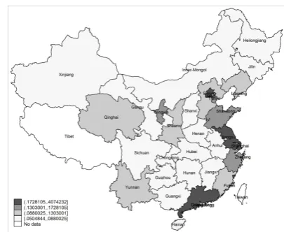
The cross-region variation in the prevalence of neighboring importers provides identification for the learning effect. Figure 1 and Figure 2 illustrate the geograph-ical distribution of the number of firms importing from the U.S., and the rate of entry into the U.S. market, respectively. These figures exhibit strong cross-regional variation in the number of importers and the market entry rate.
[Figure 1 is to be here]
[Figure 2 is to be here]
3.1. Basic Patterns
Our empirical analysis relies critically on firms’ importing activities. Table 1 re-ports statistics about the number of countries each product is imported from, and the number of products imported from each country. All statistics are at the firm-level.
The left panel of Table 1 presents statistics on the firm-level number of imported products per country. The average of the firm-level mean is 4.34 products imported per country, and the 95th percentile of the firm-level mean is 15.67. The statistics for the whole 2000-2006 period are reported first, followed by the statistics for each year between 2000-2006. The right panel of Table 1 presents the same firm-level statistics for the number of countries from which a firm imports a particular HS8 product. Consistent with our model, firms seldom import the same product from multiple countries, although they tend to import multiple products per country. In right panel, almost every statistic reported in this table is close to one. The median firm imports a single product from an average of 1 country. The last column shows that on average, around 85% firms import a single product from only one country. Similar to Antras et al. (2014), in the empirical exercise we exclude the observations where a product is imported from more than one country.
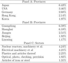
This analysis focuses primarily on the geographic and sectoral distributions of the new trade linkages established by Chinese importers over the 2000-2006 period. The empirical patterns are described in Table 2. The import entry rates exhibit destination, province, and sector diversifications. Panel A shows the top 5 desti-nations with the highest import entry rate. Japan is the destination representing 6.34% of overall import entry of Chinese firms, followed by USA, Germany, Hong Kong and Korea. Panel B reports the top 5 provinces of highest import entry rates. New imports are more concentrated in Guangdong (6.59%), and Shanghai(6.18%), followed by Jiangsu, Beijing, Liaoning. Panel C demonstrates a sectoral concen-tration of import entry. The sector of “Nuclear reactors and machinery, et al.” accounts for the highest import entry probability, 4.24% over the period in com-parison with 4.21% for “Electric machinery, et al” and 2.25% for “Plastics and articles thereof”.
4. Empirical Evidence
In this section we examine the model’s predictions using the firm-product-level import data from China.
4.1. Entry
In order to examine Proposition 1 about new importers’ entry decisions into foreign markets, we define the dependent variable of the regression as follows:
Entryicjkt = (
1 if xicjk,t−1 = 0, xicjkt >0 0 if xicjk,t−1 = 0, xicjkt >0
(26)
where Entryicjkt = 1 if firm i located in city c was not importing intermediate k from country j before yeart in the sample, but started importing k from country
j in t. xicjkt denotes firm i’s import volumes of product k from country j.
Notice first that entry is defined at firm-product-source level, and hence import source switching is treated as a new entry. For instance, if firmi imports interme-diatek from countryj′ int−1 and switches to import the same intermediate from
country j in t, Entryicjkt = 1. The reason we treat importing source switches as new entries is that switching firms do not observe the import price of a particular product in a new market. As such, they benefit from their neighbors’ information spillovers as other new importers.19 Second, since we cannot observe which firms
are the potential importers for a given intermediate, we only investigate how new importers make their import source decisions. As such, the analysis focuses on firms which import at least once during the sample period.
One difficulty in the empirical exercise is finding a measure of the signal in-ferred from neighbors, that is,µnbkj,t−1 in the model. Using the average import price
19We conduct a robustness check to investigate whether switching firms exhibit different
of k from country j revealed by neighbors to proxy the price signal could induce bias. The reason is that the firm specific searching capability is not completely observable. Therefore, an observed low import price of k in country j might re-veal neighboring importers’ strong searching capability in country j. In addition, the import price might reveal unobserved product characteristics, such as product quality. It is unclear whether a high import price implies a good or bad signal. Similar to Fernandes and Tang (2014), we use the average growth rate of existing firms’ import price of k in country j from city c between year t−1 and t as the proxy for µnbkj,t−1. This measure isolates the influence of time-invariant neighbors’ heterogeneous searching efficiency and country-product unobservable characteris-tics on the signal.20 Specifically, the neighbors’ average import price growth rate
is defined as:
∆ln(pcjkt) = 1
ncjk,t−1
X
i∈Ncjk,t−1
[ln(picjkt−lnpicjk,t−1)], (27)
whereNcjk,t−1 is the set of existing firms that import productk fromj in citycin
both yeart−1 and t, andncjk,t−1 is the number of importers in the set. Equation
(27) implies that neither new entrants in year t or one time importers in year
t−1 are included. In the baseline regressions, we also control for a wide range of fixed effects, such as city-country fixed effects, product-country fixed effects, and firm-year fixed effects to isolate the impact of time trends and other unobservable factors on firm-level import decisions.21
In order to verify that ∆ln(pcjkt) is a convincing choice of proxy for the signal, we plot the average (log) import price from countrymby firms located in regionc
in year t against the corresponding value in year t−1, after pinning down region-destination fixed effects. Figure 3 exhibits a strongly positive correlation between
20We note that price increase might indicate quality increase. We control for
country-product-year fixed effect to alleviate this concern.
21Tan et al. (2015)document the fact that more than 50% firms engaging in international
these two values. This suggests that import prices at the source and city-source level are positively correlated over time. Therefore, the import price in a market today reveals information about the import price in the same market tomorrow. Therefore, learning is profitable in the sense that import price pattern tends to be persistent.
[Figure 3 is to be here]
4.1.1. The Impact of Signals on the Firm-level Decision to Start Im-porting
Specifically, we estimate the following specification:
P r(Entryicjkt) =α+β1[ln(ncjk,t−1)∆ln(pcjkt)] +β2∆ln(pcjkt)
+β3ln(ncjk,t−1) +Z′γ+εicjkt, (28)
where Entryicjkt is defined in equation (26). The independent variables contain the proxy for the signal, ∆ln(pcjkt); the log number of neighbors in citycimporting
k from country j in the last year, and other controls including GDP per capita in the source countries,22 and a number of fixed effects. The results are reported in
Table 3.
[Table 3 is to be here]
The results in column 1 to 4 of Table 3 are obtained by adding more controls in each column. The results in column 4 indicate that the probability a firm starts importing productkfrom countryj in yeart is positively related with the number of neighbors importing k fromj in year t−1, and negatively related to the signal revealed by these neighbors. The entry decision depends on the signal more if the signal is revealed by more neighbors. More specifically, a coefficient of 0.217
22GDP per capita captures the average wage level in a particular country across all sectors.
on ln(ncjk,t−1) in column 4 implies that a one standard deviation increase in the
log number of neighbors importing from country j raises the entry probability by 2.65 percentage point. However, a coefficient of -0.083 on ∆ln(pcjkt) in column 4 suggests that at the sample mean of the observed import price growth from neighbors (12.70%) is associated with a 0.17 percentage point decrease in the probability of entry into the market.23 This number seems small, but relative to
the median entry rate in a country, which is 1.48%, a 12.70% higher growth rate in import price from a particular country is associated with a 11.49% decrease in the import entry rate. In addition, the coefficient of −0.086 on the interaction term, ln(ncjk,t−1)∆ln(pcjkt), indicates that an increase in the import price growth
among neighboring firms equal to the sample mean (12.70%), is associated with a decrease in the entry probability by 0.13 percentage points when the log number of neighbors revealing the signal increases by one standard deviation (that is, 1.37, or about 3.9 firms). This roughly explains a 9% decrease in the entry rate evaluated at the median entry rate in the sample. All the results are consistent with Proposition 1.
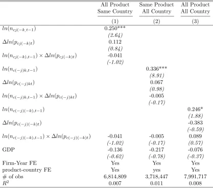
4.1.2. Different Nature of Signals
We are interested in understanding how the firm-level probability to start im-porting is related to: (1) neighboring firms which import different products from the same country (destination-specific learning); (2) neighboring firms which im-port the same product from different countries (product-specific learning); (3) neighboring firms which import different products from different countries (gener-al learning).
We define the number of neighboring firms and signals in different ways: the first is country-specific agglomeration, ln(ncj(−k),t−1), and signals ∆ln(pcj(−k),t).
These two variables denote the number of neighboring firms which import different products from the same country and the average price growth of these firms. The
23This figure is calculated following Koenig et al., (2010): −0.083×ln(1.127)×0.22×(1−
second is product-specific agglomeration ln(nc(−j)k,t−1) and signals ∆ln(pc(−j)k,t),
which capture the number of neighboring firms importing the same product from different countries and their average price growth. The last is the general agglom-eration, ln(nc(−j)(−k),t−1), and signals ∆(pc(−j)(−k),t). When calculating these two
variables, we do not take product and country into account.
All the results are reported in Table 4. Columns 1-3 report the influence of the country-specific, product-specific and general agglomeration variables and signals on firm-level decisions to start importing, respectively.
[Table 4 is to be here]
The results in Table 4 demonstrate that an increase in the number of nearby importers increases the probability that a firm starts importing no matter how how specific the agglomeration variable is constructed. In contrast, signals from these neighboring importers has an insignificant effect on firm-level decisions to start importing. One interpretation is that the price signals from different products or in various countries do not effectively reveal the price information for a particular product in an unfamiliar country. As such, we find that signal encourages entry into importing when it is highly specific, e.g. destination-product specific. However, the increase in the number of neighboring importers alone always encourages firms to start importing.
4.1.3. Heterogeneous Type of New Importers
[Table 5 is to be here]
First, Column 1 and Column 2 report our findings for firm-level decisions to start importing for a given product from a particular country across both large and small importers.24 We find that the likelihood of importing is increasing in the
number of neighboring firms importing the same product from the same country in the previous year for both types of firms. In contrast, only small firms are induced to import by the signal, and the interaction is only statistically significant for small firms. One possible explanation is that large firms have other channels to reduce uncertainties in sourcing countries, such as through incurring expensive exploration costs which are not affordable to small firms (e.g. Antras et al., 2014). Therefore, large firms do not rely on signals to make their decisions to start importing as much as small firms.
Second, Column 3 and Column 4 show the fact that while the likelihood of starting to import for heterogeneous product importers increases in the number of neighboring importers and deceases in the signal, the import probability for homo-geneous product importers only increases in the number of neighboring importers. This result is consistent with our intuition that the signal is more useful for het-erogenous product importers relative to that for homogeneous product importers due to the greater price dispersion among heterogeneous products.25
Third, Column 5 and Column 6 report the results for new importers and switch-ers. The new importers are defined as firms who did not import product k from any country j in t−1, and start importing k since t. On contrast, switchers are importers who imported productk fromj′ 6=j in yeart−1, but switch to import
the same product fromj in yeart. The results show that the number of neighbor-ing importers and the revealed signals have very similar impact on new entrants
24We classify firms into large and small categories according to their total import value in the
year they start importing.
25 Homogeneous products are more standardized and often have a reference price. These
and switchers.
Last, Column 7-9 show the results for new importers with different ownership-types, state-owned firms (SOEs), private firms and foreign-invested firms (FIEs). The results demonstrate that for firms with different ownership-types, the likeli-hood that they start importing is positively affected by the number of neighbors importing the same product from the same country in the previous year, and neg-atively related to the revealed signal. Furthermore, the signal has larger influence on the probability of importing among SOEs and private firms, when it is revealed by more neighbors. This effect is significant for FIEs only at the 90% confidence level. One possible explanation is that FIEs have better connection with foreign countries, and hence they can better identify the precision of the signal.
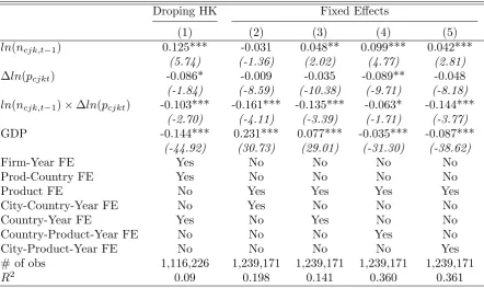
4.1.4. Robustness Checks
In this section, we conduct a series of robustness checks. We first re-estimate regression (28) by excluding imports from Hong Kong. We do this because a large share of Chinese imports from Hong Kong are imported as transit trade. Therefore, imports from Hong Kong do not reveal the import information of Hong Kong. Including these observations could potentially bias our results. The results excluding Hong Kong are reported in Column 1 of Table 6 and exhibit a similar pattern as our basic results in Table 3. Therefore, our results are not driven by the imports from Hong Kong.
shocks could potentially bias our results in Table 3. For instance, the quality of a product in a particular country might change over time. As a result, the import price and its change may partly reflect the evolution of product quality, which could bias our estimates. Using a country-product-year fixed effect, we control for this shock. The last shock we consider is a city and product specific shock. It might be the case that different cities favor importing certain kinds of products due to their own comparative advantage. We add a city-product-year fixed effect to control for this type of heterogeneity. The results with above-mentioned fixed effects are reported in column 2-6 of Table 6. It should be noted that including the various above-mentioned fixed effects in a conditional Logit model is not possible.26
Instead, following Mayneris and Poncet (2015) we use a linear probability model to estimate the firm-level import decision.
[Table 6 is to be here]
The results in Table 6 indicate that our baseline results are robust to different shocks. That is after controlling different fixed effects, the likelihood a new im-porter starts importing productk from a particular countryj in yeartis positively related to the number of neighbors importing k from j in year t−1, and nega-tively related to the signal, average import price growth as revealed by neighbors in marketj. Furthermore, the entry decision depends on the signal more so if the signal is revealed by more neighbors.
4.2. Initial Imports
4.2.1. The Impact of Signals on Firm-level Initial Imports
Proposition 2 predicts that conditional on entry, new importers’ initial imports are decreasing in the strength of the signal revealed by neighbors, and more so if
26When we attempt to control for different sets of fixed effects in a conditional Logit regression,
the large number of dummies bring computational burdens. Therefore, Mayneris and Poncet
the signal is revealed by more neighbors. We estimate equation (28) but with the entry dummy replaced by the firms’ (log) initial import quantities of k from j in year t. All subscripts have the same meaning as before. The results are reported in Table 7.
[Table 7 is to be here]
Columns (1) to (4) report the results by adding more controls in each column. The results in Column (4) indicate that initial firm-level imports are increasing in the number of neighboring importers, and decreasing in the signal only when the signal is revealed by many nearby importers. This is slightly different from the prediction in Proposition 2 in that the signal itself does affect initial firm-level imports. There are several explanations for this finding. First, as we discussed above, the signals some times are misleading, especially when they are revealed by fewer neighboring importers. As such, a portion of new importers are attracted to countries with a high import price but a revealed low expected price signal, and these misleading firms import less than expected. These misguided firms tend to obscure the effect of signals on initial firm-level imports. Second, firms often strategically choose between flexible production scheme and non-flexible scheme (see, R¨oller and Tombak, 1990; Vives, 1989). Intuitively, the more uncertainties a firm faces, the more flexible production scheme the firm chooses.27 If a signal is
revealed by more neighbors, new importers face fewer uncertainties and will choose a less flexible production scheme. In contrast, when a signal is revealed by fewer neighbors, new importers will choose a more flexible production scheme. As such, in the latter case firm-level initial imports do not rely on the signal as firms can flexibly adjust their production level and import quantities.
27Vives (1989) has shown that more flexible production schemes are more costly. Firms only
4.2.2. Different Type of Firms
In line with the section studying the decision to start importing, this section explores the effect of signals on different type of firms. All the results are reported in Table 8.
[Table 8 is to be here]
The results demonstrate that for different types of firms, the greater the number of nearby importers, the larger the initial imports from the same destinations the only exceptions are small firms and new entrants. This might be due to their production capacity, which prevents the flexibility of adjusting their import demand.
First, Column 1 and Column 2 show that relative to large firms, small firms’ initial imports are negatively affected by the signal when it is revealed by more neighboring importers (the interaction term is not statistically significant for large importers). The reason could be that large firms have better connections with foreign suppliers or local importers, etc, and hence they do not rely on the signal to help them determine how much to import.28 As such, their initial imports do
not rely on the signal.
Second, column 3 and column 4 compare the initial imports of heterogeneous product importers and homogeneous product importers. The results imply that while the initial imports for heterogeneous firms are affected by the signal when it is revealed by more neighboring firms, the initial imports for homogeneous firm-s do not depend on the firm-signal. The intuition ifirm-s that the price information for homogeneous products is easy to obtain as these products are highly standard-ized. Therefore, the signal revealed by nearby homogeneous product importers does not add as much new information as that revealed by heterogeneous product
28According toAntras et al.(2014), large firms can afford the search cost. Therefore, another
importers.
Third, Column 5 and Column 6 report the results for new importers and switch-ers. The new importers and switchers are defined in the same way as in section which studies the decisions to start importing (section 4.1.3). Interestingly, more nearby importers does not increase initial imports of new importers’ while it is significantly increasing the initial imports of switchers. In addition, although the signal has a negative impact on initial imports of both new importers and switch-ers when it is revealed by more neighboring importswitch-ers, the magnitude is much smaller for new importers. One possible explanation for these differences is that relative to switchers, the new importers might face more restrictive capacity or distributional constraints. For instance, new importers may not have established a sophisticated distributional network, and they cannot adjust their imports as flexibly as switchers due to nontrivial distributional costs. On the one hand, the neighboring importers cannot increase new importers’ initial imports. On the oth-er hand, when a good signal is revealed by more nearby importoth-ers, it only increases new importers’ initial imports in a smaller amount relative to those of switchers.
Last, we compare the response of firms with different ownership to the number of neighboring importers and signals. The results are reported in column 7-9. The results imply that an increase in the number of nearby importers will increase the initial imports for all types of firms, and the signal affects different firms only when its revealed by more nearby importers.
In sum, all of our results show that signal only play a role on initial firm-level imports when it is revealed by more neighboring importers.
4.2.3. Robustness Checks
[Table 9 is to be here]
Column 1 reports the results where we exclude firms which import from Hong Kong. Column 2-5 report the results when control for city-country-year fixed effects, city-year fixed effects, country-product-year fixed effects and city-product-year fixed effects, respectively. All results demonstrate that initial firm-level im-ports rely on signals only when they are revealed by more neighboring firms. All results are consistent with the patterns reported in Table 7.
5. Conclusions
In this paper we investigate how new importers learn from their neighbors. In con-trast to export-learning from neighbors, when a firm makes its importing decision, all markets are interdependent. The firm chooses to import each intermediate from the most attractive country, in terms of import price. However, foreign markets are associated with a high-level of uncertainty relative to the domestic market. This feature encourages new importer to learn from their neighboring importers in order to reduce the uncertainty in foreign markets.
We build an economic model to rationalize firm-level import-learning from neighbors. New firms have prior beliefs about the prices in foreign markets. Their entry and initial import decisions rely on their beliefs of the import prices. New firms can update their prior beliefs by observing signals revealed by their neigh-boring importers
The model predicts that an increase in the number of neighboring firms import-ing product k from country j increases both the probability that new importers start importing the same product from the same country, and increases their ini-tial imports. In addition, a good signal revealed by neighboring importers also encourages entry and increases initial imports. This effect is particularly strong when the signal is revealed by a greater number of neighbors.
countryj in yeart is increasing in the number of nearby firms importing the same product from the same country in yeart−1, and decreasing in the signal about the market’s expected price inferred from neighbors’ import performance. The latter effect is particularly strong if the signal is revealed by more neighbors. Second, the results demonstrate that the initial firm-level imports are increasing in the number of nearby firms importing the same product from the same country, and decreasing in the signal only when the signal is revealed by more neighbors.
Reference
Ahn, J., Khandelwal, A.K., and Wei, S.J., 2011. The Role of Intermediaries in Facilitating Trade. Journal of International Economics, 84, 73–85.
Aitken, B., and Harrison, A.E. 1997. Spillovers, Foreign Investment, and Export Behavior Journal of International Economics, 43, 103-132.
Allen, T.,Forthcomming. Information Frictions in Trade. Econometrica.
Khandelwal, Amit, Schott, Peter, and Wei, S.J., 2013. Trade Liberalization and Embedded Institutional Reform: Evidence from Chinese Exporters. American Economic Review, 103, 2169-95.
Antras, P., and Staiger, R., 2012. Offshoring and the Role of Agreements. Amer-ican Economic Review, 107, 3140-3183.
Antras, P., Fort, C. Teresa, and Tintelnot, Felix 2014. The Margins of Global Sourcing: Theory and Evidence From U.S. Firms. Working Paper.
Arkolakis, C., 2010. Market Penetration Costs and the New Consumers Margin in International Trade. Journal of Political Economy, 118, 1151-1199.
Bas, M., and V. Strauss-Kahn, 2015. Input-Trade Liberalization, Export Prices and Quality Upgrading. Journal of International Economics, 95, 250-262.
Bergin, P., Feenstra, R. and Hanson, H. 2011. Volatility Due To Offshoring: Theory and Evidence. Journal of International Economics 85, 163-173.
Bernard, A.B.,J. Bradford S. Redding, and P. Schott, 2009. The Margins of US Trade. American Economic Review, 99, 487–493.
Bernard, A.B., Redding, S.J., and Schott, P.K., 2011. Multiproduct Firms and Trade Liberalization. The Quarterly Journal of Economics, 126, 1271–1318.
Bernard, A.B., and J. Jensen, Why Do Firms Export. The Review of Economics and Statistics, 86, 561–569.
Cassey, A.J. and Schmeiser, K.N., 2013. The Agglomeration of Exporters by Destination. The Annals of Region Science, 51, 495-513.
Chaney, T., 2014. A Network Structure of International Trade. American Eco-nomic Review, 104, 3600-3634.
Clerides, S.K., Lach, S. and Tybout, J., 1998. Is Learning by Exporting Importan-t? Micro-Dynamic Evidence from Colombia, Mexico, and Morocco. Quarterly Journal of Economics, 113, 903-947.
Dasgupta, K. and Mondria, J., 2014. Inattentive Importers.University of Toronto, Mimeo.
DeGroot, M.H., 2004. Optimal Statistic Decisions. Wiley-Interscience, 82
Demidova, S., Kee, H.L. and Krishna, K., 2011. Do Trade Policy Differences Induce Sorting? Theory and Evidence From Bangledeshi Apparel Exporters. NBER Working Paper , 12725.
Eaton, Jonathan and Kortum, Samuel 2002. Technology, Geography, and Trade. Econometrica, 70, 1741-1779.
Eaton, Jonathan, Eslava, M., and Kugler, M. 2008. The Margins of Entry into Export Markets: Evidence from Columbia. In: Helpman, Elhanan, Marin, Dalia, Verdier, Thierry (Eds.), The Organization of Firms in a Global Economy. Harvard University Press, Cambridge, MA,, p.2008.
Ethier, W. 1982. National and International Returns to Scale in the Modern Theory of International Trade American Economic Review, 72, 389-405.
Feng, L., Z.Li and D.Swenson 2016. The Connection between Imported Intermedi-ate Inputs and Exports: Evidence from Chinese Firms.Jounrnal of International Economics, 101, 86-101.
Fernandes, A.P. and Tang, H. 2014. Learning to Export from Neighbors Journal of International Economics, 94, 67-84.
Goldberg, P., A. Khandelwal, N. Pancnik and P. Topaloval 2010. Imported In-termediate Inputs and Domestic Product Growth: Evidence From India The Quarterly Journal of Economics, 125, 1727-1767.
Koenig, P., Mayeris, F., and Poncet, S., 2010. Local Export Spillovers in France. European Economic Review, 54, 622-641.
Hu, C., Z. Xu, and N. Yashiro, 2015. Agglomeration and Productivity in China: Firm Level Evidence. China Economics Review, 33, 50-66.
Kneller, R. and Pisu, M., 2007. Industrial Linkages and Export Spillovers from FDI. The World Economy, 30(1), 105-134.
Koenig, P., Mayeris, F., and Poncet, S., 2010. Local Export Spillovers in France. European Economic Review, 54, 622-641.
Krautheim, S., 2008. Gravity and Information: Heterogeneous Firms, Exporters Networks and ‘Distance Puzzle’. EUI Mimeo
R¨oller, L., and M. Tombak, 1990. Strategic Choice of Flexible Production Tech-nologies and Welfare Implications. The Journal of Industrial Economics, , 38(4), 417-431.
Lin, H., H. Li, and C. Yang, 2011. Agglomeration and Productivity: Firm-Level Evidence from China’s Textile Industry. China Economic Review, , 22, 313-329.
Manova, K., and Zhang, Z., 2012. Multi-Product Firms and Product Quality. NBER Working Papers, 18637.
Mayneris, F., and Poncet, S., 2015. Chinese Firms’ Entry to Export Markets: the Role of Foreign Export Spillovers. World Bank Economic Review, 29(1), 150-179.
Melitz, M. 2003. The Impact of Trade on Intra-Industry Reallocations and Aggre-gate Industry Productivity. Econometrica. 71, 1695–1725.
Nocke, V., Yeaple, S.R., 2014. Globalization and Multiproduct Firms. Interna-tional Economic Review 55, 993-1018.
Portes, R. and Rey, H., 2005. The Determinants of Cross-Border Equity Flows. Journal of International Economics, 65, 269-296.
Puhani, P, 2012. The Treatment Effect, the Cross Difference, and the Interaction term in Nonlinear “Difference-in-Differences” Models. Economics Letters, 115, 85-87.
Ramanarayanan, Ananth 2006. International Trade Dynamics with International Inputs. mimeo University of Mnnesota.
Rauch, J.E., 1999. Networks Versus Markets in International Trade. Journal of International Economics, 48, 7-35.
Rauch, J.E. and Watson, J., 2003. Starting Small in an Unfamiliar Enviroment. International Journal of Industrial Organization, 21, 1021-1042.
Steinwender, C., 2014. When the States and the Kingdom Become United. mimeo, London School of Economics
Taiji, F.,Ito, K.,Inui, T. and Tang, H. 2015. Offshoring, Relationship-Specificity, and Domestic Production. Working Paper
Rotunno, L., Vezina, P.L., and Wang, Z., 2013. The Rise and Fall of (Chinese) African Apparel Exports. Journal of Development Economics, , 105, 152-163.
Vives, X., 1989. Technological Competition, Uncertainty, and Oligopoly. Journal of Econoic Theory, , 48, 386-415.
Yang, C., H. Lin, and H. Li, 2013. Influences of Production and R&D Agglomera-tion on Productivity: Evidence from Chinese Electrics Firms. China Economic Review, , 27, 162-178.
Yeats, A. 2001. Just How Big Is Global Production Sharing? In Arnt, Sven W., and Kierzkowski, Henry eds.,, Fragmentation: New Production Patterns in the World Economy. Oxford University Press
Appendix (Figures and Tables)
[image:40.595.302.505.386.552.2]Num. Neighbors (US) 2001 Num. Neighbors (US) 2006
Figure 1
[image:40.595.89.287.387.554.2]The rate of entry into U.S. Market 2001 The rate of entry into U.S. Market 2006
Table 1: Firm-Level Statistics on the Number of Imported Products per Source Country and the Number of Source Countries per Imported Product
products per country countries per product The ratio of firm-level firm-level imported product mean median max mean median max from single country 2000-2006
mean 4.34 3.49 9.13 1.16 1.08 1.79
median 2.00 1.71 2.57 1.00 1.00 1.00 82.92% 95%tile 15.67 12.42 39.28 1.91 1.57 5.00
2000
mean 4.07 3.31 8.38 1.14 1.06 1.71
median 2.00 1.50 2.00 1.00 1.00 1.00 83.36% 95%tile 14.33 11.50 35 1.79 1.50 5.00
2001
mean 4.26 3.46 8.86 1.15 1.07 1.75
median 2.00 2.00 3.00 1.00 1.00 1.00 82.84% 95%tile 15.00 12.00 37.00 1.85 1.50 5.00
2002
mean 4.52 3.64 9.48 1.15 1.07 1.78
median 2.00 2.00 3.00 1.00 1.00 1.00 83.16% 95%tile 16.25 13.00 40.00 1.85 1.50 5.00
2003
mean 4.56 3.64 9.76 1.16 1.07 1.81
median 2.00 2.00 3.00 1.00 1.00 1.00 83.29% 95%tile 16.50 13.00 42.00 1.93 1.50 5.00
2004
mean 4.51 3.61 9.58 1.17 1.08 1.81
median 2.00 1.50 3.00 1.00 1.00 1.00 83.24% 95%tile 16.66 13.00 42.00 2.00 1.50 5.00
2005
mean 4.37 3.50 9.23 1.17 1.08 1.79
median 2.00 1.50 2.00 1.00 1.00 1.00 83.23% 95%tile 16.66 12.50 41.00 2.00 1.50 5.00
2006
mean 4.10 3.29 8.64 1.21 1.11 1.86
median 2.00 1.50 2.00 1.00 1.00 1.00 81.34% 95%tile 15.00 12.00 38.00 2.00 2.00 5.00