Munich Personal RePEc Archive
Bayesian multivariate Beveridge–Nelson
decomposition of I(1) and I(2) series
with cointegration
Murasawa, Yasutomo
Konan University
5 February 2019
Bayesian multivariate Beveridge–Nelson
decomposition of I(1) and I(2) series with
cointegration
∗
Yasutomo Murasawa
Faculty of Economics, Konan University
8-9-1 Okamoto, Higashinada-ku, Kobe, Hyogo 658-8501, Japan
First draft: December 2018
This version: February 5, 2019
Summary
The consumption Euler equation implies that the output growth rate and the real interest rate are of the same order of integration; thus if the real inter-est rate is I(1), then so is the output growth rate with possible cointegration, and log output is I(2). This paper extends the multivariate Beveridge–Nelson decomposition to such a case, and develops a Bayesian method to obtain error bands. The paper applies the method to US data to estimate the natural rates (or their permanent components) and gaps of output, inflation, interest, and unemployment jointly, and finds that allowing for cointegration gives much bigger estimates of all gaps.
Keywords Natural rate, Output gap, Trend–cycle decomposition, Trend inflation, Unit root, Vector error correction model (VECM)
JEL classification C11, C32, C82, E32
1
INTRODUCTION
Distinguishing between growth and cycles is fundamental in macroeconomics. One
can define growth as the time-varying steady state, or the permanent component,
and cycles as deviations from the steady state, or the transitory component. One
may interpret the permanent and transitory components as the natural rate and
gap, respectively, though some economists may disagree with such interpretation, in
which case one can consider the permanent component of the natural rate.1 If shocks
affecting the two components differ, then policy prescriptions for promoting growth
and stabilizing cycles differ. Thus it is useful to decompose economic fluctuations
into the two components.
Among such decomposition methods, this paper focuses on the multivariate
Beveridge–Nelson (B–N) decomposition, which decomposes a multivariate I(1) or
CI(1,1) series into a random walk permanent component and an I(0) transitory
component, assuming a linear time series model such as a VAR model or a
vec-tor error-correction model (VECM) for the differenced series. In practice, however,
some series may be I(2), e.g., log output in some countries, in which case one must
decompose I(1) and I(2) series jointly. Murasawa (2015) develops the multivariate
B–N decomposition of I(1) and I(2) series.
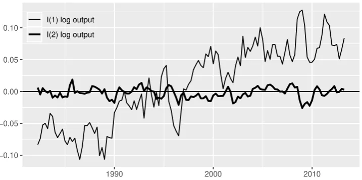
As Murasawa (2015) shows, for non-US data, the B–N decomposition assuming
I(1) log output often gives an unreasonable estimate of the output gap, perhaps
because of possible structural breaks in the mean output growth rate; see Figure 1.
Kamber, Morley, and Wong (2018, p. 563) explain,
. . . if there is a large reduction in the long-run growth rate, a forecasting
model that fails to account for it will keep anticipating faster growth
1
than actually occurs after the break, leading to a persistently negative
estimate of the output gap based on the BN decomposition.2
Assuming I(2) log output and hence I(1) output growth rate, one introduces a
stochastic trend in the output growth rate, which captures possible structural breaks
in the mean growth rate automatically in real time without specifying break dates
a priori. Thus the B–N decomposition assuming I(2) log output gives a more
“rea-sonable” estimate of the output gap that fluctuates around 0; see Figure 1.
Figure 1
This paper extends Murasawa (2015) in two ways. First, we allow for
cointegra-tion in the multivariate B–N decomposicointegra-tion of I(1) and I(2) series. Recall that the
consumption Euler equation in a simple macroeconomic model implies a dynamic
IS equation such that for allt,
Et(∆yt+1) =
1
σ(rt−ρ) (1)
whereyt is log output,rt is the real interest rate,ρ is the discount rate, andσ is the
curvature of the utility of consumption; see Gal´ı (2015, pp. 21–23). This equation
implies that if 0< σ < ∞, then the output growth rate and the real interest rate are of the same order of integration; thus if the real interest rate is I(1), then so
is the output growth rate with possible cointegration, and log output is I(2). This
observation motivates our development of the multivariate B–N decomposition of
I(1) and I(2) series with cointegration.
Second, we apply Bayesian analysis to obtain error bands for the components,
building on recent developments in Bayesian analysis of a VECM. Since cointegrating
2
In this quote, Kamber et al. (2018) seem to consider theoutput growth rate gap. If one fails to account for a large reduction in the true mean growth rateµ∗, then the output growth rate ∆yttends to be below the assumed mean growth rateµ; i.e., the output growth rate gap ∆yt−µ
indeed tends to be negative. If log output is I(1), so that the output growth rate is I(0), then with positive serial correlation, the future ∆yt−µtends to be negative, implying that the current
vectors require normalization, our parameter of interest is in fact the cointegrating
space rather than cointegrating vectors. Strachan and Inder (2004) use a matrix
angular central Gaussian (MACG) distribution proposed by Chikuse (1990) as a
prior on the cointegrating space. Koop, Le´on-Gonz´alez, and Strachan (2010) propose
a collapsed Gibbs sampler for posterior simulation of such a model. Since one often
has prior information on the steady state of a system, Villani (2009) specifies a
prior on the steady state form of a VECM. Since some hyperparameters such as the
tightness (shrinkage) hyperparameter on the VAR coefficients are difficult to choose,
Giannone, Lenza, and Primiceri (2015) use a hierarchical prior. We utilize these
ideas, and show how to simulate the joint posterior distribution of the components.
As an application, we simulate the joint posterior distribution of the natural
rates (or their permanent components) and gaps of output, inflation, interest, and
unemployment in the US during 1950Q1–2017Q4. To apply the Bayesian
multi-variate B–N decomposition of I(1) and I(2) series with cointegration, we assume
a four-variate VAR model for the output growth rate, the CPI inflation rate, the
short-term interest rate, and the unemployment rate, and estimate it in the VECM
form. The Bayes factors give decisive evidences that the cointegrating rank is 2. The
posterior medians of the gaps seem reasonable compared to previous works that
fo-cus on a particular natural rate or gap. The posterior probability of positive gap is
useful when the sign of the gap is uncertain. The Phillips curve and Okun’s law hold
between the gaps, though we do not impose such relations. Comparisons of
alterna-tive model specifications show not only that assuming I(2) log output gives a more
“reasonable” estimate of the output gap, but also that allowing for cointegration
gives much bigger estimates of all gaps.
The paper proceeds as follows. Section 2 reviews the literature on the B–N
decomposition. Section 3 derives the multivariate B–N decomposition of I(1) and
I(2) series with cointegration. Section 4 specifies our model and prior, and explains
data. Section 6 discusses remaining issues. The Appendix gives the details of the
derivation of our algorithm.
2
LITERATURE
Beveridge and Nelson (1981) give operational definitions of the permanent and
tran-sitory components, show that one can express any I(1) series as the sum of a random
walk permanent component and an I(0) transitory component, and propose the B–N
decomposition of a univariate I(1) series, assuming an ARIMA model.3
Multivariate extension of the B–N decomposition is straightforward. Evans
(1989a, 1989b) and Evans and Reichlin (1994) apply the B–N decomposition to
a multivariate series consisting of I(0) and I(1) series, assuming a VAR model for
the stationarized series. Evans and Reichlin (1994) show that the transitory
compo-nents are no smaller with the multivariate B–N decomposition than with the
univari-ate one. This is because the transitory components are “forecastable movements”
(Rotemberg and Woodford (1996)), and multivariate models forecast no worse than
univariate models, using more information. King, Plosser, Stock, and Watson (1991)
and Cochrane (1994) apply the B–N decomposition to a CI(1,1) series, assuming a
VECM.
J. C. Morley (2002) gives a general framework for the B–N decomposition,
us-ing a state space representation of the assumed linear time series model. Garratt,
Robertson, and Wright (2006) note that if the state vector is observable as in a VAR
model or a VECM, then the transitory component is an explicit weighted sum of the
observables given the model parameters; thus the multivariate B–N decomposition
based on a VAR model or a VECM is transparent. They also note that the result of
the multivariate B–N decomposition depends strongly on the assumed cointegrating
rank.
3
The B–N decomposition also applies to an I(2) series. Newbold and Vougas
(1996), Oh and Zivot (2006), and Oh, Zivot, and Creal (2008) extend the B–N
decomposition to a univariate I(2) series. Murasawa (2015) extends the method to
a multivariate series consisting of I(1) and I(2) series.
One can apply Bayesian analysis to obtain error bands for the components. This
approach is useful especially when the state vector is observable as in a VAR model
or a VECM, in which case the components are explicit functions of the model
param-eters and observables; thus the joint posterior distribution of the model paramparam-eters
directly translates into that of the components. Murasawa (2014) uses a Bayesian
VAR model to obtain error bands for the components.
Kiley (2013) uses a Bayesian DSGE model, but gives no error band for the
com-ponents. Del Negro et al. (2017) use a Bayesian DSGE model and give error bands
for the components. They also use a multivariate unobserved components (UC)
model, where the permanent components have a factor structure and the transitory
components follow a VAR model. Bayesian analysis of a UC model requires state
smoothing, since the state vector is unobservable given the model parameters; thus
it is less straightforward than that of a VAR model. J. Morley and Wong (2018) use
a large Bayesian VAR model and give error bands for the components, but they do
not take parameter uncertainty into account. There seems no previous work that
uses a Bayesian VECM to obtain error bands for the components.4
4
3
MODEL SPECIFICATION
3.1
VAR model
Let ford = 1,2, {xt,d} be an Nd-variate I(d) sequence. Let N :=N1+N2. Let for
allt, xt:= (x′t,1,xt,′2)′, yt,1 :=xt,1, yt,2 := ∆xt,2, and yt:= (yt,′1,y′t,2)′, so that {yt}
is I(1). Assume also that{yt}is CI(1,1) with cointegrating rankr. Let ford= 1,2,
µd := E(∆yt,d). Let µ:= (µ′1,µ′2)′. Let {y∗t} be such that for all t,
yt=α+µt+y∗t (2)
Assume a VAR(p+ 1) model for {yt∗}such that for all t,
Π(L)yt∗ =ut (3)
{ut} ∼WN(Σ) (4)
3.2
VECM representation
Write
Π(L) =Π(1)L +Φ(L)(1−L)
where Φ(L) := (Π(L)−Π(1)L)/(1−L). Then we have a VECM of order p for
{∆y∗
t}such that for all t,
Φ(L)∆yt∗ =−Π(1)y∗t−1+ut
=−ΛΓ′yt∗−1+ut (5)
where Λ,Γ ∈ RN×r. Since {y∗t} is CI(1,1), the roots of det(Π(z)) = 0 must lie on or outside the unit circle. This requirement gives an implicit restriction on the
We can write for allt,
Φ(L)(∆yt−µ) =−ΛΓ′[yt−1 −α−µ(t−1)] +ut
=−Λ[Γ′yt−1 −β−δ(t−1)] +ut (6)
where β := Γ′α and δ := Γ′µ. Though slightly different, the last expression is
essentially a steady state VECM suggested by Villani (2009, p. 633). We have for
allt,
E(∆yt) =µ (7)
E(Γ′yt) =β+δt (8)
which help us to specify an informative prior on (µ,β,δ). Thus a steady state
VECM is useful for Bayesian analysis.
3.3
State space representation
Assume that p≥1. We have for all t,
Γ′yt∗ =Γ′(yt∗−1+Φ1∆yt∗−1 +· · ·+Φp∆yt∗−p−ΛΓ′yt∗−1+ut)
=Γ′Φ1∆yt∗−1+· · ·+Γ′Φp∆yt∗−p+ (Ir−Γ′Λ)Γ′y∗t−1+Γ′ut
or
Γ′yt−β−δt=Γ′Φ1(∆yt−1−µ) +· · ·+Γ′Φp(∆yt−p−µ)
Letst be a state vector such that for all t,
st:=
∆yt−µ
... ∆yt−p+1−µ Γ′yt−β−δt
which is I(0) and observable given the model parameters. A state space
representa-tion of the steady state VECM is for all t,
st=Ast−1 +Bzt (10)
∆yt=µ+Cst (11)
{zt} ∼WN(IN) (12)
where A:=
Φ1 . . . Φp −Λ
I(p−1)N O(p−1)N×N O(p−1)N×r
Γ′Φ1 . . . Γ′Φp Ir−Γ′Λ
B:=
Σ1/2
O(p−1)N×N
Γ′Σ1/2 C := [
IN ON×(p−1)N ON×r
]
Note that{st} is I(0) if and only if the eigenvalues of Alie inside the unit circle. We have for all t, for h≥0,
or
Et(∆xt+h,1) = µ1 +C1Ahst (13)
Et
(
∆2xt+h,2 )
=µ2 +C2Ahst (14)
where
C1 :=
[
IN1 ON1×N2 ON1×(p−1)N ON1×r
]
C2 :=
[
ON2×N1 IN2 ON2×(p−1)N ON2×r
]
3.4
Multivariate B–N decomposition
Introducing cointegration changes the state space model, but the formulae for the
multivariate B–N decomposition of I(1) and I(2) series given by Murasawa (2015,
Theorem 1) remain almost unchanged. Let x∗t and ct be the B–N permanent and
transitory components inxt, respectively.
Theorem 1. Suppose that the eigenvalues of A lie inside the unit circle. Then for
all t,
x∗t,1 = lim
T→∞(Et(xt+T,1)−Tµ1) (15)
x∗t,2 = lim
T→∞
{
Et(xt+T,2)−T2 µ2
2 −T
[µ 2
2 + ∆xt,2+C2(IpN+r−A)
−1As
t
]}
(16)
ct,1 =−C1(IpN+r−A)−1Ast (17)
ct,2 =C2(IpN+r−A)−2A2st (18)
Proof. See Murasawa (2015, pp. 158–159).
Let
W :=
−C1(IpN+r−A)−1A
C2(IpN+r−A)−2A2
Then for all t,
ct=W st (19)
where W depends only on the VECM coefficients and {st} is observable given the model parameters. This observation is useful for Bayesian analysis of{ct}.
4
BAYESIAN ANALYSIS
4.1
Conditional likelihood function
Assume Gaussian innovations for Bayesian analysis, and write the VECM as for all
t,
∆yt−µ=Φ1(∆yt−1−µ) +· · ·+Φp(∆yt−p−µ)
−Λ[Γ′yt−1−β−Γ′µ(t−1)] +ut (20)
{ut} ∼INN
(
0N,P−1
)
(21)
Letψ:= (β′,µ′)′,Φ:= [Φ
1, . . . ,Φp], andY := [y0, . . . ,yT]. By the prediction error
decomposition, the joint pdf of Y is
p(Y|ψ,Φ,P,Λ,Γ) = p(∆yT, . . . ,∆yp+1,sp|ψ,Φ,P,Λ,Γ)
=
T
∏
t=p+1
p(∆yt|st−1,ψ,Φ,P,Λ,Γ)p(sp|ψ,Φ,P,Λ,Γ) (22)
Our Bayesian analysis relies on ∏T
t=p+1p(∆yt|st−1,ψ,Φ,P,Λ,Γ), the conditional
likelihood function of (ψ,Φ,P,Λ,Γ) givensp.
4.2
Identification
To specify a prior on the cointegrating space, we assume that Γ′Γ = I
r. This
then we can apply linear normalization. WriteΓ := [Γ1′,Γ2′]′, where Γ1 is r×r and
Γ2 is (N −r)×r. Let
¯
Λ:=ΛΓ1
¯
Γ :=Γ Γ1−1
Then we can identify ( ¯
Λ,Γ¯). Let ¯β := ¯Γ′α= (
Γ1−1)′β and ¯ψ := (¯
β′,µ′)′
corre-spondingly. Note thatα is not identifiable from the VECM.
4.3
Prior
4.3.1 Steady state parameters
Assume a normal prior on (α,µ) independent of (Φ,P,Λ,Γ) such that
α µ
∼N2N α0 µ0 ,
Q−0,1α ON×N
ON×N Q−0,1µ
(23)
Sinceβ :=Γ′α, this prior implies a prior onψ such that
ψ|Γ ∼Nr+N
(
ψ0,Q−01 )
(24)
where
ψ0 :=
Γ′α0
µ0
, Q0 :=
(
Γ′Q−0,1αΓ)−1 Or×r ON×N Q0,µ
which depends onΓ in general.5 The joint pdf of ψ is
p(ψ) = (2π)−(r+N)/2det(Q0)1/2exp
(
−1
2(ψ−ψ0)
′Q0(ψ−ψ0)
)
(25)
5
4.3.2 VAR parameters
LetS be the set of (Φ,Λ,Γ) such that the eigenvalues ofAlie inside the unit circle,
so that {yt∗} is CI(1,1). Assume a hierarchical normal–Wishart prior on (Φ,P) independent ofψ but dependent on (Λ,Γ) such that
Φ|P, ν,Λ,Γ ∼NN×pN
(
M0;P−1,(νD0)−1 )
[(Φ,Λ,Γ)∈S] (26)
P ∼WN
(
k0;S0−1 )
(27)
ν ∼Gam
(
A0
2 ,
B0
2
)
(28)
where ν is a hyperparameter that controls the tightness of the prior on the VAR
coefficients, which is often difficult to choose a priori, and we assume a gamma prior
onν. The joint pdf of (Φ,P, ν) conditional on (Λ,Γ) is
p(Φ,P, ν|Λ,Γ) =p(Φ|P, ν,Λ,Γ)p(P)p(ν) (29)
where
p(Φ|P, ν,Λ,Γ) = etr(−P(Φ−M0)νD0(Φ−M0)
′/2)
(2π)pN2/2
det(νD0)−N/2det(P)−pN/2[(Φ,Λ,Γ)∈S] (30)
p(P) = det(P)
(k0−N−1)/2/etr((S0/2)P)
ΓN(k0/2) det(S0/2)−k0/2
(31)
p(ν) = ν
A0/2−1/e(B0/2)ν
Γ(A0/2)(B0/2)−A0/2
(32)
where ΓN(.) is theN-variate gamma function. See Gupta and Nagar (1999) on the
pdfs of the matrix normal and Wishart distributions.
4.3.3 Cointegrating space
LetVr
(
RN) be the r-dimensional Steifel manifold in RN, i.e.,
Vr
(
RN):={
H ∈RN×r :H′H =Ir
Its volume is
Vol(
Vr
(
RN))= 2
rπN r/2
Γr(N/2)
(33)
See Muirhead (1982, p. 70). Following Strachan and Inder (2004), we assume a prior
not on the elements ofΓ directly but onVr
(
RN). Let H0 ∈Vr
(
RN). Let H(.) be s.th. ∀τ ≥0,
H(τ) :=H0H0′ +τH0⊥H0′⊥
so that H(0) = H0H0′ is of rank r and H(1) = IN. Assume a prior on (Λ,Γ)
conditionally independent of (ψ,P) givenΦ such that6
Λ|Γ,Φ∼NN×r
(
Λ0;G−01,(Γ′η0H(τ0)Γ)−1 )
[(Φ,Λ,Γ)∈S] (34)
Γ|Φ∼MACGN×r
(
H(τ0)−1 )
(35)
The joint pdf of (Λ,Γ) conditional onΦ is
p(Λ,Γ|Φ) =p(Λ|Γ,Φ)p(Γ|Φ) (36)
where
p(Λ|Γ,Φ) = etr(−G0(Λ−Λ0)Γ
′η0H(τ
0)Γ(Λ−Λ0)′/2)
(2π)N r/2det(Γ′η
0H(τ0)Γ)−N/2det(G0)−r/2
[(Φ,Λ,Γ)∈S] (37)
p(Γ|Φ) = det(Γ
′H(τ
0)Γ)−N/2/det(H(τ0))−r/2
Vol(Vr(RN))
(38)
Ifτ0 := 1, thenp(Γ) = 1/Vol (
Vr
(
RN)), i.e., the flat prior onΓ. See Chikuse (1990) on the MACG distribution.
6
Apart from the restriction that (Φ,Λ,Γ)∈S, if τ0 := 1, then sinceΓ′Γ =Ir, the prior on
The following transformation is useful for posterior simulation. Let
Λ∗ := (Λ−Λ0)[(Λ−Λ0)′(Λ−Λ0)]−1/2
Γ∗ :=Γ[(Λ−Λ0)′(Λ−Λ0)]1/2
Then Λ∗Γ∗′ = (Λ−Λ0)Γ′ and Γ∗′Γ∗ = (Λ−Λ0)′(Λ−Λ0). Following Koop et al.
(2010, p.230), we have
p(Λ,Γ|Φ) =p(Λ∗,Γ∗|Φ)
=p(Γ∗|Λ∗,Φ)p(Λ∗|Φ) (39)
where
Γ∗|Λ∗,Φ∼NN×r
(
ON×r; (η0H(τ0))−1,(Λ′∗G0Λ∗)−1
)
[(Φ,Λ∗,Γ∗)∈S] (40)
Λ∗|Φ∼MACGN×r
( G−01)
(41)
so that
p(Γ∗|Λ∗,Φ) =
etr(−η0H(τ0)Γ∗Λ′∗G0Λ∗Γ∗/2)
(2π)N r/2det(Λ′
∗G0Λ∗)−N/2det(η0H(τ0))−r/2
[(Φ,Λ∗,Γ∗)∈S] (42)
p(Λ∗|Φ) =
det(Λ′∗G0Λ∗)−N/2/det(G0)−r/2
Vol(Vr(RN))
(43)
This is essentially because
p(Λ|Γ,Φ)p(Γ|Φ)∝etr
(
−1
2G0(Λ−Λ0)Γ
′η0H(τ
0)Γ(Λ−Λ0)′ )
[(Φ,Λ,Γ)∈S]
= etr
(
−1
2G0Λ∗Γ
′
∗η0H(τ0)Γ∗Λ′∗
)
[(Φ,Λ∗,Γ∗)∈S]
= etr
(
−1
2η0H(τ0)Γ∗Λ
′
∗G0Λ∗Γ∗′
)
4.4
Posterior simulation
We simulate p(ψ,Φ,P,Λ,Γ, ν|Y) by a Gibbs sampler consisting of five blocks:
1. Draw ψ fromp(ψ|Φ,P,Λ,Γ, ν,Y) = p(ψ|Φ,P,Λ,Γ,Y).
2. Draw (Φ,P) from p(Φ,P|ψ,Λ,Γ, ν,Y).
3. Draw Λ from p(Λ|ψ,Φ,P,Γ, ν,Y) = p(Λ|ψ,Φ,P,Γ,Y). Let Λ∗ := (Λ−
Λ0)[(Λ−Λ0)′(Λ−Λ0)]−1/2.
4. Draw Γ∗ from p(Γ∗|ψ,Φ,P,Λ, ν,Y) = p(Γ∗|ψ,Φ,P,Λ,Y). Discard Λ. Let
Γ :=Γ∗(Γ∗′Γ∗)−1/2 andΛ:=Λ0+Λ∗(Γ∗′Γ∗)1/2. Accept the draw if (Φ,Λ,Γ)∈
S; otherwise go back to step 2 and draw another (Φ,P,Λ,Γ).
5. Draw ν from p(ν|ψ,Φ,P,Λ,Γ,Y) =p(ν|Φ,P).
The first block builds on Villani (2009); the second block is standard; the third
and fourth blocks come from the collapsed Gibbs sampler proposed by Koop et al.
(2010); the fifth block is standard. See the Appendix for the details of each block.
4.5
Bayes factor
We use the Bayes factor for Bayesian model selection. When choosing between
nested models with certain priors, the Savage–Dickey (S–D) density ratio gives
the Bayes factor without estimating the marginal likelihoods; see Wagenmakers,
Lodewyckx, Kuriyal, and Grasman (2010) for a tutorial on the S–D method.
We choose the cointegrating rankr. Consider comparing the following two
mod-els (hypotheses):
H0 : rk(Π) = 0 vs Hr : rk(Π) =r (44)
Koop, Le´on-Gonz´alez, and Strachan (2008, pp. 451–452) note that the problem is
the same as comparing the following two nested models:
Ignoring the constraint that (Φ,Λ,Γ) ∈ S for the moment and assuming that
τ0 := 1, so that the priors onΛ and Γ are independent,7 the S–D density ratio for
H0 vs Hr is
B0,r =
p(Λ=ON×r|Y;Hr)
p(Λ=ON×r|Hr)
(46)
The prior gives the denominator directly. For the numerator, we have
p(Λ|Y;Hr) = E(p(Λ|ψ,Φ,P,Γ,Y;Hr)|Y;Hr) (47)
Let{ψl,Φl,Pl,Γl}Ll=1 be posterior draws. Let
ˆ
p(Λ =ON×r|Y;Hr) :=
1
L
L
∑
l=1
p(Λ=ON×r|ψl,Φl,Pl,Γl,Y;Hr)
An estimator of the the S–D density ratio forH0 vs Hr is
ˆ
B0,r =
ˆ
p(Λ=ON×r|Y;Hr)
p(Λ=ON×r|Hr)
(48)
5
APPLICATION
5.1
Data
We consider joint estimation of the natural rates (or their permanent components)
and gaps of the following four macroeconomic variables in the US:
Output LetYt be output. Assume that{lnYt} is I(2), so that {∆ lnYt} is I(1).
Inflation rate LetPtbe the price level andπt:= ln(Pt/Pt−1) be the inflation rate.
Assume that {πt} is I(1).
Interest rate LetItbe the 3-month nominal interest rate (annual rate in per cent),
it := ln(1 +It/400), rt :=it−Et(πt+1) be the ex ante real interest rate, and
7
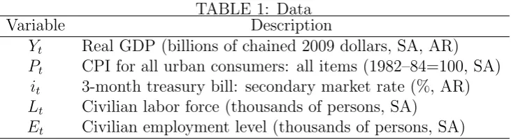
TABLE 1: Data
Variable Description
Yt Real GDP (billions of chained 2009 dollars, SA, AR)
Pt CPI for all urban consumers: all items (1982–84=100, SA)
it 3-month treasury bill: secondary market rate (%, AR)
Lt Civilian labor force (thousands of persons, SA)
Et Civilian employment level (thousands of persons, SA)
Note: SA means ‘seasonally-adjusted’; AR means ‘annual rate’.
ˆ
rt :=it−πt+1 be the ex post real interest rate. Assume that {rt} is I(1).8
[image:19.595.206.383.456.555.2]Unemployment rate Let Lt be the labor force, Et be employment, and Ut := −ln(Et/Lt) be the unemployment rate. Assume that {Ut} is I(1).
Table 1 describes the data, which are available from FRED (Federal Reserve
Economic Data). When monthly series are available, i.e., except for real GDP, we
take the 3-month arithmetic means of monthly series each quarter to obtain quarterly
series, from which we construct the quarterly inflation, interest, and unemployment
rates as defined above.
Let for all t,
xt:=
πt ˆ rt Ut
lnYt
, yt:=
πt ˆ rt Ut
∆ lnYt
The sample period of {yt} is 1948Q1–2017Q4 (280 observations).
5.2
Preliminary analyses
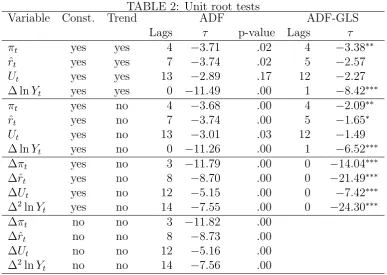
We perform some preliminary analyses to check our assumption that{yt} is I(1).9
Table 2 shows the results of the ADF and ADF-GLS tests for unit root, with or
without constant and/or trend terms in the ADF regression. The results depend on
8
We can estimate the interest rate gap even if we observe{ˆrt}instead of{rt}. See Murasawa (2014, pp. 499–500).
9
TABLE 2: Unit root tests
Variable Const. Trend ADF ADF-GLS Lags τ p-value Lags τ
πt yes yes 4 −3.71 .02 4 −3.38∗∗
ˆ
rt yes yes 7 −3.74 .02 5 −2.57
Ut yes yes 13 −2.89 .17 12 −2.27
∆ lnYt yes yes 0 −11.49 .00 1 −8.42∗∗∗
πt yes no 4 −3.68 .00 4 −2.09∗∗
ˆ
rt yes no 7 −3.74 .00 5 −1.65∗
Ut yes no 13 −3.01 .03 12 −1.49
∆ lnYt yes no 0 −11.26 .00 1 −6.52∗∗∗
∆πt yes no 3 −11.79 .00 0 −14.04∗∗∗
∆ˆrt yes no 8 −8.70 .00 0 −21.49∗∗∗
∆Ut yes no 12 −5.15 .00 0 −7.42∗∗∗
∆2lnY
t yes no 14 −7.55 .00 0 −24.30∗∗∗
∆πt no no 3 −11.82 .00
∆ˆrt no no 8 −8.73 .00
∆Ut no no 12 −5.16 .00
∆2lnY
t no no 14 −7.56 .00
Note: For the ADF-GLS test, *, **, and *** denote significance at the 10%, 5%, and 1% levels, respectively. For the number of lags included in the ADF
regression, we use the default choice in gretl 2018d with maximum 15, where the lag order selection criteria are AIC for the ADF test, and a modified AIC using the Perron and Qu (2007) method for the ADF-GLS test. With no constant nor trend in the ADF regression, the ADF test is asymptotically point optimal; hence the ADF-GLS test is unnecessary.
the number of lags included in the ADF regression, since the ADF test suffers from
size distortion with short lags and low power with long lags. The ADF-GLS test
remedies the problem except when there is no constant nor trend term in the ADF
regression, in which case the ADF test is asymptotically point optimal. The level
.05 ADF-GLS test rejects H0 : {yt,i} ∼ I(1) in favor of H1 : {yt,i} ∼ I(0) for {πt}
and{∆ lnYt}. Hence these unit root tests do not support our assumption that {yt}
is I(1).
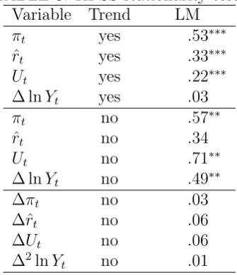
Table 3 shows the results of the KPSS stationarity tests, with or without a trend
term. The results depend on the lag truncation parameter for the Newey–West
estimator of the long-run error variance. With a trend term, the level .05 KPSS test
TABLE 3: KPSS stationarity tests Variable Trend LM
πt yes .53∗∗∗
ˆ
rt yes .33∗∗∗
Ut yes .22∗∗∗
∆ lnYt yes .03
πt no .57∗∗
ˆ
rt no .34
Ut no .71∗∗
∆ lnYt no .49∗∗
∆πt no .03
∆ˆrt no .06
∆Ut no .06
∆2lnY
t no .01
Note: ** and *** denote significance at the 5% and 1% levels, respectively. The lag truncation parameter for the Newey–West estimator of the long-run error variance is 5 (the default value for our sample length in gretl 2018d).
trend term, the test rejectsH0 :{yt,i} ∼I(0) in favor ofH1 :{yt,i} ∼I(1) except for {ˆrt}. Though the results for {rˆt} and {∆ lnYt} are mixed, these stationarity tests
support our assumption that {yt}is I(1).
Overall, these unit root and stationarity tests confirm that {∆yt} is I(0), but are inconclusive if each component of{yt}is I(1). With no strong counter-evidence, we proceed with our prior belief that each component of{yt}is I(1). See Murasawa (2014) for an analysis based on an alternative assumption.
We also perform some preliminary analyses of cointegration in {yt}. Table 4 shows the results of the Engle–Granger cointegration tests, with or without a trend
term in the cointegrating regression. The results depend on the number of lags
included in the ADF regression for the residual series, but overall, the tests fail to
reject the null of no cointegration (the residual series is I(1)) against the alternative
of cointegration (the residual series is I(0)).
Table 5 shows the results of Johansen’s cointegration tests, with unrestricted
constant and restricted trend terms in the VECM. The results depend on the number
TABLE 4: Engle–Granger cointegration tests Trend τ p-value
yes −3.75 .22 no −3.56 .17
[image:22.595.175.411.239.313.2]Note: The number of lags included in the ADF regression is 4 (the default value for our sample length in gretl 2018d).
TABLE 5: Johansen’s cointegration tests (unrestricted constant and restricted trend in the VECM)
Rank Trace p-value λ-max p-value 0 141.91 .00 83.45 .00 1 58.46 .00 40.08 .00 2 18.39 .33 12.50 .38 3 5.89 .48 5.89 .49
Note: The number of lags included in the VECM is 4 (the default value for our sample length in gretl 2018d).
rank is 2.
Since the results are mixed, we estimate models with different cointegrating
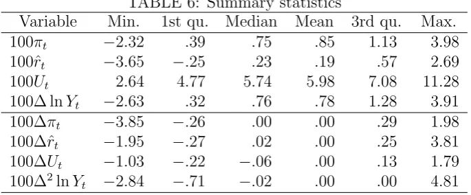
ranks, and use the Bayes factor to choose the cointegrating rank. Table 6 shows
summary statistics of{yt} and {∆yt} multiplied by 100. Note that{πt},{rˆt}, and
{∆ lnYt} are quarterly rates of change (not annualized).
5.3
Model specification
For our data, N := 4. To select p, we fit VAR models to {yt} up to VAR(8), i.e., p = 7, and check model selection criteria. The common estimation period is
TABLE 6: Summary statistics
Variable Min. 1st qu. Median Mean 3rd qu. Max. 100πt −2.32 .39 .75 .85 1.13 3.98
100ˆrt −3.65 −.25 .23 .19 .57 2.69
100Ut 2.64 4.77 5.74 5.98 7.08 11.28
100∆ lnYt −2.63 .32 .76 .78 1.28 3.91
100∆πt −3.85 −.26 .00 .00 .29 1.98
100∆ˆrt −1.95 −.27 .02 .00 .25 3.81
100∆Ut −1.03 −.22 −.06 .00 .13 1.79
100∆2lnY
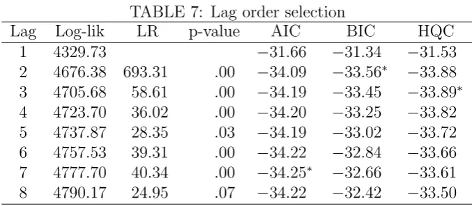
[image:22.595.127.470.613.755.2]TABLE 7: Lag order selection
Lag Log-lik LR p-value AIC BIC HQC 1 4329.73 −31.66 −31.34 −31.53 2 4676.38 693.31 .00 −34.09 −33.56∗ −33.88
3 4705.68 58.61 .00 −34.19 −33.45 −33.89∗
4 4723.70 36.02 .00 −34.20 −33.25 −33.82 5 4737.87 28.35 .03 −34.19 −33.02 −33.72 6 4757.53 39.31 .00 −34.22 −32.84 −33.66 7 4777.70 40.34 .00 −34.25∗ −32.66 −33.61
8 4790.17 24.95 .07 −34.22 −32.42 −33.50
Note: For AIC, BIC, and HQC, * denotes the selected model. The LR test
statistic for testing H0 :{yt} ∼VAR(p−1) vsH1 :{yt} ∼VAR(p) follows χ2(16)
underH0.
1950Q1–2017Q4. Table 7 summarizes the results of lag order selection.10 The level
.05 LR test fails to rejectH0 :{yt} ∼VAR(7) againstH1 :{yt} ∼VAR(8) and AIC
selects VAR(7), whereas BIC and HQC select much smaller models. Since a
high-order VAR model covers low-high-order VAR models as special cases, to be conservative,
we assume a VAR(8) model for {yt}, i.e., we choosep= 7, and impose a shrinkage
prior on the VAR coefficients.
For the prior on α, we set α0 := 0N and Q0,α := IN; hence the prior on β is
Nr(0r,Ir) independent of Γ. For the prior on µ, we set µ0 := ˆµ, where ˆµ is the
sample mean of{∆ lnyt}, and Q0,µ :=IN.
Following Kadiyala and Karlsson (1997) and Ba´nbura, Giannone, and Reichlin
(2010), we set
M0 :=ON×pN
D0 := diag(1, . . . , p)2⊗diag(s1, . . . , sN)2
k0 :=N + 2
S0 := (k0−N −1) diag(s1, . . . , sN)2
10
where fori= 1, . . . , N,s2
i is an estimate of var(ut,i) based on the univariate AR(p+1)
model with constant and trend terms for{yt,i}.
For the prior on (Λ,Γ), we set Λ0 := ON×r, G0 :=IN, η0 := .01, and τ0 := 1.
Since τ0 := 1, we have a flat prior on the cointegrating space, and the priors on Λ
and Γ are independent.
For the prior onν, we setA0 := 1 andB0 := 1, i.e.,ν ∼χ2(1); hence the tightness
hyperparameter on the VAR coefficients tends to be small, implying potentially mild
shrinkage toward M0 :=ON×pN.
Overall, our priors are weakly informative in the sense of Gelman et al. (2014,
p. 55).
5.4
Bayesian computation
We run our Gibbs sampler on R 3.5.2 developed by R Core Team (2018). We use
the ML estimate of (Φ,P,Λ,Γ) for their initial values.11 With poor initial values,
the restriction that the eigenvalues of A lie inside the unit circle does not hold,
and the iteration cannot start. Hence the choice of initial values is important when
one applies the B–N decomposition. Once the iteration starts, the restriction rarely
binds for our sample.
To check convergence of the Markov chain generated by our Gibbs sampler to its
stationary distribution, we perform convergence diagnoses discussed in Robert and
Casella (2009, ch. 8) and available in the coda package for R. Given the diagnoses,
we discard the initial 1,000 draws, and use the next 4,000 draws for the posterior
inference.
To select the cointegrating rank r, we set p := 7, assume the above priors,
and compute the S–D density ratios for r = 1,2,3, from which we compute the
posterior probabilities of r = 0,1,2,3, assuming equal prior probabilities. We find
that the posterior probability of r = 2 is numerically 1, consistent with the results
11
of Johansen’s cointegration tests. Thus we setr := 2 in the following analysis.
5.5
Empirical results
Figure 2 plots the actual rates and our point estimates (posterior medians) of the
natural rates (or their permanent components) of the four variables. For ease of
comparison of the actual and natural rates, we omit error bands for the natural
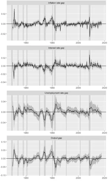
rates, which are identical to those for the gaps. Figure 3 plots our point estimates
of the gaps and their 95% error bands.
Figure 2
Figure 3
Our estimate of the natural rate of inflation is smoother than typical univariate
estimates of trend inflation in the CPI; e.g., Faust and Wright (2013, p. 22). It
looks close to a recent estimate of trend inflation in the US CPI in J. Morley,
Piger, and Rasche (2015, p. 894) based on a bivariate UC model for the inflation
and unemployment rates, which assumes independent shocks to the trend and gap
components and allows for structural breaks in the variances of these shocks. It is
more volatile, however, than a recent estimate of trend inflation in the PCE price
index by Chan, Clark, and Koop (2018, p. 21) that uses information in survey
inflation expectations.
Our estimate of the natural rate of interest is more volatile than a recent estimate
by Del Negro et al. (2017, p. 237) based on a VAR model with common trends, i.e.,
a multivariate UC model with independent shocks to the trend and gap components
and a factor structure for the trend components, for short- and long-term interest
rates, inflation and its survey expectations, and some other variables. Their estimate
is smooth partly because they impose tight priors on the variances of the shocks to
the trend components. Indeed, their estimate with the loosest possible prior is as
on a DSGE model looks close to ours despite different definitions of the natural rate;
see Del Negro et al. (2017, p. 237).12 Estimates by Laubach and Williams (2016,
p. 60), Holston et al. (2017, p. S61), and Lewis and Vazquez-Grande (2019) are
close to trend output growth by construction, and quite different from estimates by
Del Negro et al. (2017) and ours, especially before 1980.13
Our estimate of the natural rate of unemployment looks more volatile than a
recent estimate in J. Morley et al. (2015, p. 898), obtained as a by-product of
esti-mation of trend inflation. A possible reason for the difference is that they assume
independent shocks to the trend and gap components, which may not hold in
prac-tice. If one allows for dependence between the shocks, then the two estimates may
coincide, as J. C. Morley, Nelson, and Zivot (2003) show for the univariate trend–
cycle decomposition. Our estimate of the unemployment rate gap looks close to
the estimate in J. Morley et al. (2015, p. 901) in terms of the sign and magnitude,
despite the difference in the volatility.
Our estimate of the output gap is at most about ±5% of the output level, and looks close to a recent estimate by J. Morley and Wong (2018, Fig. 2) based on a
large Bayesian VAR(4) model with 23 variables. It also looks close to their estimate
based on a Bayesian VAR(4) model with four variables using output growth, the
unemployment rate, the CPI inflation rate, and the growth rate of industrial
pro-duction, assuming that they are all I(0). Though output growth may or may not be
I(0) in the US, it may be clearly I(1) in some countries or regions, in which case their
method may give an unreasonable estimate of the output gap with a strong upward
or downward trend. See Murasawa (2015) for such an example for the Japanese
data.
12
Del Negro et al. (2017) clearly distinguish the natural rate and its low-frequency component, estimating the former by a DSGE model and the latter by a VAR model.
13
Holston et al. (2017, p. S63) writes,
. . . we assume a one-for-one relationship between the trend growth rate of output and the natural rate of interest, which corresponds to assumingσ= 1 in Eq. (1).
Figure 4 plots the posterior probability of positive gap for the four variables.
This probability index is useful if the sign of the gap is of interest. Even if the 95%
error band for the gap covers 0, the posterior probability of positive gap may be
close to .025 or .975. Indeed, the probability index is often below .25 or above .75;
hence we are often quite sure about the sign of the gap. Moreover, Figure 4 shows
the relation between the gaps more clearly than Figure 3.
Figure 4
Figure 5 shows the relation between the gaps more directly. The left panels are
the scatter plots of the posterior medians of the gaps in each quarter. The right
panels are the posterior pdfs of the correlation coefficients between the gaps. We
see that the Phillips curves and Okun’s law hold between the gaps, though we do
not impose such relations. Thus our estimates of the gaps seem mutually consistent
from a macroeconomic point of view.
Figure 5
5.6
Comparison of alternative model specifications
Figure 6 compares point estimates of the gaps under three alternative assumptions,
i.e., I(1) log output, I(2) log output with no cointegration, and I(2) log output with
cointegration. For ease of comparison, we omit error bands here.
Figure 6
The result assuming I(1) log output is similar to that in Murasawa (2014), who
uses a VAR model with no constant term for the differenced and centered series, sets
p:= 12, and chooses the tightness hyperparameter by the empirical Bayes method.
In contrast to the result for the Japanese data in Murasawa (2015), for the US data,
the multivariate B–N decomposition assuming I(1) log output gives “reasonable”
Assuming I(2) log output with no cointegration changes the estimate of the
output gap, but hardly changes the estimates of other gaps, which is similar to the
result for the Japanese data in Murasawa (2015). In particular, the output gap now
keeps fluctuating around 0 since 2010, which seems more “reasonable”.
Allowing for cointegration changes the estimates of all gaps, and we obtain much
bigger gaps. The result makes sense because the B–N transitory components are
“forecastable movements”, and a VECM forecasts better than a VAR model,
espe-cially for our data. Moreover, these bigger gaps seem close to other recent estimates
that focus on a particular gap, as already noted.
6
DISCUSSION
The consumption Euler equation implies that if the real interest rate is I(1), then
so is the output growth rate with possible cointegration, and log output is I(2).
We extend the multivariate B–N decomposition to such a case. To obtain error
bands for the components, we apply Bayesian analysis. In particular, we assume
hierarchical weakly informative priors, and develop a Gibbs sampler for posterior
simulation. Application of the method to US data gives a reasonable joint estimate
of the natural rates (or their permanent components) and gaps of output, inflation,
interest, and unemployment.
The B–N decomposition assuming I(1) log output often gives an unreasonable
estimate of the output gap, perhaps because of possible structural breaks in the
mean output growth rate. Assuming I(2) log output, i.e., I(1) output growth rate,
we introduce a stochastic trend in the output growth rate, which captures possible
structural breaks in the mean growth rate automatically in real time without
spec-ifying break dates a priori, leading to a more reasonable estimate of the output gap
that fluctuates around 0. Moreover, since the B–N transitory components are
for cointegration gives larger estimates of all gaps.
Since a reduced-form VECM is the most basic forecasting model for cointegrated
series, the multivariate B–N decomposition based on a VECM gives a benchmark
joint estimate of the natural rates (or their permanent components) and gaps. One
can compare this benchmark estimate with alternative estimates based on other
forecasting models or DSGE models such as those in Del Negro et al. (2017). We
conjecture that our method is useful especially for non-US data, where log output is
often clearly I(2). Confirming this conjecture is an interesting and important issue
for future work.
One can possibly refine our estimate in two ways. First, one can use a larger
model with more variables, assuming a factor structure if necessary. Second, one
can introduce Markov-switching, stochastic volatility, or more general time-varying
parameters to our VECM. Since the B–N decomposition may not apply to nonlinear
models, and nonlinear models may become unnecessary with more variables, the first
direction seems more promising.
Lastly, to obtain a monthly instead of quarterly joint estimate of the natural
rates and gaps of output and other variables, it seems straightforward to extend the
B–N decomposition of mixed-frequency series proposed by Murasawa (2016) to I(1)
and I(2) series with cointegration.
REFERENCES
Ba´nbura, M., Giannone, D., & Reichlin, L. (2010). Large Bayesian vector auto
regressions. Journal of Applied Econometrics, 25, 71–92. doi: 10.1002/
jae.1137
Beveridge, S., & Nelson, C. R. (1981). A new approach to decomposition of economic
time series into permanent and transitory components with particular
7, 151–174. doi: 10.1016/0304-3932(81)90040-4
Chan, J. C. C., Clark, T. E., & Koop, G. (2018). A new model of inflation, trend
inflation, and long-run inflation expectations. Journal of Money, Credit and
Banking,50, 5–53. doi: 10.1111/jmcb.12452
Chikuse, Y. (1990). The matrix angular central Gaussian distribution. Journal of
Multivariate Analysis, 33, 265–274. doi: 10.1016/0047-259X(90)90050-R
Cochrane, J. H. (1994). Permanent and transitory components of GNP and
stock prices. Quarterly Journal of Economics, 109, 241–265. doi: 10.2307/
2118434
Cogley, T., Morozov, S., & Sargent, T. J. (2005). Bayesian fan charts for U.K.
inflation: Forecasting and sources of uncertainty in an evolving monetary
system. Journal of Economic Dynamics and Control, 29, 1893–1925. doi:
10.1016/j.jedc.2005.06.005
Cogley, T., Primiceri, G. E., & Sargent, T. J. (2010). Inflation-gap persistence
in the US. American Economic Journal: Macroeconomics, 2, 43–69. doi:
10.1257/mac.2.1.43
Cogley, T., & Sargent, T. J. (2002). Evolving post-World War II U.S. inflation
dynamics. NBER Macroeconomics Annual 2001,16, 331–373. doi: 10.1086/
654451
Cogley, T., & Sargent, T. J. (2005). Drifts and volatilities: Monetary policies and
outcomes in the post WWII US. Review of Economic Dynamics, 8, 262–302.
doi: 10.1016/j.red.2004.10.009
Del Negro, M., Giannone, D., Giannoni, M. P., & Tambalotti, A. (2017). Safety,
liquidity, and the natural rate of interest. Brookings Papers on Economic
Activity, 48(1), 235–316.
Dr`eze, J. H., & Richard, J.-F. (1983). Bayesian analysis of simultaneous equation
systems. In Z. Griliches & M. D. Intriligator (Eds.), Handbook of econometrics
Evans, G. W. (1989a). A measure of the U.S. output gap. Economics Letters, 29,
285–289. doi: 10.1016/0165-1765(89)90202-4
Evans, G. W. (1989b). Output and unemployment dynamics in the United States:
1950–1985. Journal of Applied Econometrics, 4, 213–237. doi: 10.1002/
jae.3950040302
Evans, G. W., & Reichlin, L. (1994). Information, forecasts, and measurement
of the business cycle. Journal of Monetary Economics, 33, 233–254. doi:
10.1016/0304-3932(94)90002-7
Faust, J., & Wright, J. H. (2013). Forecasting inflation. In G. Elliott & A.
Timmer-mann (Eds.), Handbook of economic forecasting (Vol. 2A, pp. 2–56). Elsevier.
doi: 10.1016/b978-0-444-53683-9.00001-3
Gal´ı, J. (2015). Monetary policy, inflation, and the business cycle(2nd ed.).
Prince-ton University Press.
Garratt, A., Robertson, D., & Wright, S. (2006). Permanent vs transitory
com-ponents and economic fundamentals. Journal of Applied Econometrics, 21,
521–542. doi: 10.1002/jae.850
Gelman, A., Carlin, J. B., Stern, H. S., Dunson, D. B., Vehtari, A., & Rubin, D. B.
(2014). Bayesian data analysis (3rd ed.). CRC Press.
Giannone, D., Lenza, M., & Primiceri, G. E. (2015). Prior selection for vector
autoregressions. Review of Economics and Statistics, 97, 436–451. doi: 10
.1162/rest a 00483
Gupta, A. K., & Nagar, D. K. (1999).Matrix variate distributions. Taylor & Francis
Ltd.
Holston, K., Laubach, T., & Williams, J. C. (2017). Measuring the natural rate
of interest: International trends and determinants. Journal of International
Economics, 108, S59–S75. doi: 10.1016/j.jinteco.2017.01.004
Kadiyala, K. R., & Karlsson, S. (1997). Numerical methods for estimation and
99–132. doi: 10.1002/(SICI)1099-1255(199703)12:2<99::AID-JAE429>3
.0.CO;2-A
Kamber, G., Morley, J., & Wong, B. (2018). Intuitive and reliable estimates of
the output gap from a Beveridge–Nelson filter. Review of Economics and
Statistics, 100, 550–566. doi: 10.1162/rest a 00691
Kiley, M. T. (2013). Output gaps. Journal of Macroeconomics, 37, 1–18. doi:
10.1016/j.jmacro.2013.04.002
Kilian, L., & L¨utkepohl, H. (2017). Structural vector autoregressive analysis.
Cam-bridge University Press.
King, R., Plosser, C., Stock, J., & Watson, M. (1991). Stochastic trends and
economic fluctuations. American Economic Review, 81, 819–840.
Koop, G. (2003). Bayesian econometrics. John Wiley & Sons.
Koop, G., Le´on-Gonz´alez, R., & Strachan, R. W. (2008). Bayesian inference in a
cointegrating panel data model. In S. Chib, W. Griffiths, G. Koop, & D. Terrell
(Eds.),Bayesian econometrics (Vol. 23, pp. 433–469). Emerald. doi: 10.1016/
s0731-9053(08)23013-6
Koop, G., Le´on-Gonz´alez, R., & Strachan, R. W. (2010). Efficient posterior
simu-lation for cointegrated models with priors on the cointegration space.
Econo-metric Reviews,29, 224–242. doi: 10.1080/07474930903382208
Laubach, T., & Williams, J. C. (2016). Measuring the natural rate of interest redux.
Business Economics,51, 57–67. doi: 10.1057/be.2016.23
Lewis, K. F., & Vazquez-Grande, F. (2019). Measuring the natural rate of interest:
A note on transitory shocks. Journal of Applied Econometrics. (in press) doi:
10.1002/jae.2671
Morley, J., Piger, J., & Rasche, R. (2015). Inflation in the G7: Mind the gap(s)?
Macroeconomic Dynamics,19, 883–912. doi: 10.1017/s1365100513000655
Morley, J., & Wong, B. (2018, September). Estimating and accounting for the
Paper Series No. 2018-4). University of Sydney.
Morley, J. C. (2002). A state-space approach to calculating the Beveridge–
Nelson decomposition. Economics Letters, 75, 123–127. doi: 10.1016/
s0165-1765(01)00581-x
Morley, J. C., Nelson, C. R., & Zivot, E. (2003). Why are the Beveridge–Nelson
and unobserved-components decompositions of GDP so different? Review of
Economics and Statistics,85, 235–243. doi: 10.1162/003465303765299765
Muirhead, R. J. (1982). Aspects multivariate statistic theory. John Wiley & Sons.
Murasawa, Y. (2014). Measuring the natural rates, gaps, and deviation cycles.
Empirical Economics, 47, 495–522. doi: 10.1007/s00181-013-0747-9
Murasawa, Y. (2015). The multivariate Beveridge–Nelson decomposition with I(1)
and I(2) series. Economics Letters, 137, 157–162. doi: 10.1016/j.econlet
.2015.11.001
Murasawa, Y. (2016). The Beveridge–Nelson decomposition of mixed-frequency
series. Empirical Economics,51, 1415–1441. doi: 10.1007/s00181-015-1061
-5
Nelson, C. R. (2008). The Beveridge–Nelson decomposition in retrospect and
prospect. Journal of Econometrics, 146, 202–206. doi: 10.1016/j.jeconom
.2008.08.008
Newbold, P., & Vougas, D. (1996). Beveridge–Nelson-type trends for I(2) and
some seasonal models. Journal of Time Series Analysis, 17, 151–169. doi:
10.1111/j.1467-9892.1996.tb00270.x
Oh, K. H., & Zivot, E. (2006, January).The Clark model with correlated components.
(unpublished) doi: 10.2139/ssrn.877398
Oh, K. H., Zivot, E., & Creal, D. (2008). The relationship between the Beveridge–
Nelson decomposition and other permanent–transitory decompositions that
are popular in economics. Journal of Econometrics, 146, 207–219. doi: 10
Perron, P., & Qu, Z. (2007). A simple modification to improve the finite sample
properties of Ng and Perron’s unit root tests. Economics Letters. doi: 10
.1016/j.econlet.2006.06.009
Phelps, E. S. (1995). The origins and further development of the natural rate of
unemployment. In R. Cross (Ed.), The natural rate of unemployment:
Re-flections on 25 years of the hypothesis (pp. 15–31). Cambridge University
Press.
R Core Team. (2018). R: A language and environment for statistical computing
[Computer software manual]. Vienna, Austria. Retrieved from https://www
.R-project.org/
Robert, C. P., & Casella, G. (2009). Introducing Monte Carlo methods with R.
Springer.
Rotemberg, J. J., & Woodford, M. (1996). Real-business-cycle models and the
fore-castable movements in output, hours, and consumption. American Economic
Review,86, 71–89.
Strachan, R. W., & Inder, B. (2004). Bayesian analysis of the error correction model.
Journal of Econometrics, 123, 307–325. doi: 10.1016/j.jeconom.2003.12
.004
Verdinelli, I., & Wasserman, L. (1995). Computing Bayes factors using a
general-ization of the Savage–Dickey density ratio. Journal of the American Statistical
Association,90, 614–618. doi: 10.1080/01621459.1995.10476554
Villani, M. (2009). Steady-state priors for vector autoregressions.Journal of Applied
Econometrics, 24, 630–650. doi: 10.1002/jae.1065
Wagenmakers, E.-J., Lodewyckx, T., Kuriyal, H., & Grasman, R. (2010). Bayesian
hypothesis testing for psychologists: A tutorial on the Savage–Dickey method.
Cognitive Psychology,60, 158–189. doi: 10.1016/j.cogpsych.2009.12.001
A
APPENDIX: GIBBS SAMPLER
A.1
Useful lemmas
Our Gibbs sampler relies on the following two familiar results in Bayesian analysis
of normal linear models, which we state as lemmas for ease of reference.
Lemma 1. Suppose that
y=Xβ+u
u∼Nn
(
0n,P−1
)
and
β ∼Nk
(
µ0,D0−1 )
Then
β|P,y,X ∼Nk
(
µ1,D1−1 )
where
D1 :=X′P X+D0
µ1 :=D−11(X′P XbGLS+D0µ0)
with bGLS := (X′P X)−1X′P y.
Proof. See Koop (2003, pp. 118–121).
Lemma 2. Suppose that
Y =XB′+U
U ∼Nn×m
(
On×m;In,P−1
and
B|P ∼Nm×k
(
M0;P−1,D0−1 )
P ∼Wm
(
k0;S0−1 )
Then
B|P,Y,X ∼Nm×k
(
M1;P−1,D−11)
P|Y,X ∼Wm
(
k1;S1−1 )
where
D1 :=X′X+D0
M1 := (BOLSX′X+M0D0)D1−1
k1 :=n+k0
S1 := (BOLS−M0) [
(X′X)−1+D−1 0
]−1
(BOLS−M0)′ +S +S0
with BOLS :=Y′X(X′X)−1 and S := (Y −XB′
OLS)′(Y −XBOLS′ ).
Proof. See Dr`eze and Richard (1983, pp. 539–541).
A.2
Steady state parameters
Write the VECM as for allt,
Φ(L)∆yt−Φ(1)µ=−Λ[Γ′yt−1−β−Γ′µ(t−1)] +ut
or
Let for allt,
wt:=Φ(L)∆yt+ΛΓ′yt−1
Zt:=
[
Λ Φ(1) + (t−1)ΛΓ′ ]
Then for all t,
wt=Ztψ+ut
Let w:=
wp+1
... wT
, Z :=
Zp+1
... ZT
, u:=
up+1
... uT
Then we have a normal linear model for w given Z such that
w =Zψ+u (50)
u ∼NN(T−p) (
0N(T−p),(IT−p⊗P)−1
)
(51)
LetψGLS:= [Z′(IT−p⊗P)Z]−1Z′(IT−p⊗P)w.
Theorem 2.
ψ|Φ,P,Λ,Γ,w∼Nr+N
(
ψ1,Q−11 )
(52)
where
Q1 :=Z′(IT−p ⊗P)Z+Q0
ψ1 :=Q−11[Z′(IT−p⊗P)ZψGLS+Q0ψ0]
A.3
VAR parameters
Let for allt,
et:=Γ′yt−β−δt, s∗t :=
∆yt−µ
... ∆yt−p+1−µ
Write the VECM as for allt,
∆yt−µ+Λet−1 =Φs∗t−1+ut (53)
Let
Y∗ :=
(∆yp+1−µ+Λep)′
...
(∆yT −µ+ΛeT−1)′
, X :=
s∗′ p ...
s∗′T−1
, U :=
u′ p+1 ...
u′T
Then we have a normal linear model for Y∗ given X such that
Y∗ =XΦ′+U (54)
U ∼N(T−p)×N
(
O(T−p)×N;IT−p,P−1
)
(55)
LetΦOLS:=Y∗′X(X′X)−1 and S := (Y∗−XΦ′OLS)′(Y∗ −XΦ′OLS).
Theorem 3.
Φ|P,ψ,Λ,Γ, ν,Y∗,X ∼NN×pN
(
M1;P−1,D−11)[(Φ,Λ,Γ)∈S] (56)
P|ψ,Λ,Γ, ν,Y∗,X ∼WN
(
k1;S1−1 )
where
D1 :=X′X+νD0
M1 := (ΦOLSX′X+M0νD0)D−11
k1 :=T −p+k0
S1 := (ΦOLS−M0) [
(X′X)−1+ (νD0)−1 ]−1
(ΦOLS−M0)′+S +S0
Proof. Apply Lemma 2.
A.4
Loading matrix
Write the VECM as for allt,
Φ(L)(∆yt−µ) =−Λet−1+ut (58)
Let W :=
[Φ(L)(∆yp+1−µ)]′
...
[Φ(L)(∆yT −µ)]′
, E:=
−e′
p
...
−e′
T−1
Then we have a normal linear model for W given E such that
W =EΛ′+U
U ∼N(T−p)×N
(
O(T−p)×N;IT−p,P−1
)
or
W′ =ΛE′+U′
U′ ∼NN×(T−p) (
ON×(T−p);P−1,IT−p
Letλ:= vec(Λ). Then we have a normal linear model for vec(W′) such that
vec(W′) = (E⊗IN)λ+ vec(U′) (59)
vec(U′)∼NN(T−p) (
0N(T−p),IT−p ⊗P−1
)
(60)
Letλ0 := vec(Λ0) and
U0 :=Γ′η0H(τ0)Γ ⊗G0
so that
λ|Γ,Φ∼NN r
(
λ0,U0−1)[(Φ,Λ,Γ)∈S] (61)
Theorem 4.
λ|ψ,Φ,P,Γ,W,E ∼NN r
(
λ1,U1−1 )
[(Φ,Λ,Γ)∈S] (62)
where
U1 =E′E⊗P +U0 (63)
λ1 =U1−1vec(P W′E+G0Λ0Γ′η0H(τ0)Γ) (64)
Proof. LetΛOLS :=W′E(E′E)−1 and λOLS:= vec(ΛOLS). By Lemma 1,
U1 := (E⊗IN)′(IT−p⊗P)(E⊗IN) +U0
=E′E⊗P +U0
where
(E′E⊗P)λOLS = (E′E⊗P) vec (
W′E(E′E)−1)
= (E′E⊗P)[
(E′E)−1 ⊗W′]vec(E)
= (Ir⊗P W′) vec(E)
= vec(P W′E)
U0λ0 = (Γ′η0H(τ0)Γ ⊗G0) vec(Λ0)
= vec(G0Λ0Γ′η0H(τ0)Γ)
A.5
Cointegrating matrix
Write the VECM as for allt,
Φ(L)(∆yt−µ)−Λβ =−Λ∗Γ∗′[yt−1−µ(t−1)] +ut (65)
Let
W∗ :=
[Φ(L)(∆yp+1−µ)−Λβ]′
...
[Φ(L)(∆yT −µ)−Λβ]′
, Z∗ :=
−(yp−pµ)′
...
−[yT−1−(T −1)µ]′
Then we have a normal linear model for W∗ given Z∗ such that
W∗ =Z∗Γ∗Λ′∗+U
U ∼N(T−p)×N
(
O(T−p)×N;IT−p,P−1
Letγ∗ := vec(Γ∗). Then we have a normal linear model for vec(W∗) such that
vec(W∗) = (Λ∗⊗Z∗)γ∗ + vec(U) (66)
vec(U)∼NN(T−p) (
0N(T−p),P−1⊗IT−p
)
(67)
Let
V0 :=Λ′∗G0Λ∗⊗η0H(τ0)
so that
γ∗|Λ∗,Φ∼NN r
(
0N r,V0−1 )
[(Φ,Λ∗,Γ∗)∈S] (68)
Theorem 5.
γ∗|ψ,Φ,P,Λ∗,W∗,Z∗ ∼NN r
(
γ1,V1−1 )
[(Φ,Λ∗,Γ∗)∈S] (69)
where
V1 =Λ′∗P Λ∗⊗Z∗′Z∗+V0 (70)
γ1 =V1−1vec(Z∗′W∗P Λ∗) (71)
Proof. Letγ∗,GLS be the GLS estimator of γ∗, i.e.,
γ∗,GLS= [(Λ∗⊗Z∗)′(P ⊗IT−p)(Λ∗⊗Z∗)]−1(Λ∗⊗Z∗)′(P ⊗IT−p) vec(W∗)
By Lemma 1,
V1 := (Λ∗⊗Z∗)′(P ⊗IT−p)(Λ∗⊗Z∗) +V0
=Λ′∗P Λ∗⊗Z∗′Z∗+V0
γ1 :=V1−1(Λ′∗P Λ∗⊗Z∗′Z∗)γ∗,GLS
=V1−1(Λ′∗P ⊗Z∗′) vec(W∗)
=V1−1vec(Z∗′W∗P Λ∗)
A.6
Tightness hyperparameter
We have
p(ν|ψ,Φ,P,Λ,Γ,Y)
∝p(Y|ψ,Φ,P,Λ,Γ, ν)p(ψ|Φ,P,Λ,Γ, ν)p(Λ,Γ|Φ,P, ν)p(Φ,P|ν)p(ν)
=p(Y|ψ,Φ,P,Λ,Γ)p(ψ|Φ,P,Λ,Γ)p(Λ,Γ|Φ,P)p(Φ,P|ν)p(ν)
∝p(Φ,P|ν)p(ν)
Thusp(ν|ψ,Φ,P,Λ,Γ,Y) = p(ν|Φ,P).
Theorem 6.
ν|Φ,P ∼Gam
(
A1
2 ,
B1
2
)
(72)
where
A1 :=pN2+A0
Proof. The result follows because
p(Φ,P|ν)p(ν)∝νpN2/2etr
(
−P(Φ−M0)νD0(Φ−M0)
′
2
)
νA0/2−1
e(B0/2)ν
= ν
(pN2
+A0)/2−1
−0.10 −0.05 0.00 0.05 0.10
1990 2000 2010
I(1) log output
I(2) log output
[image:45.595.120.479.303.481.2]Log output Unemployment rate
Real interest rate Inflation rate
1960 1980 2000 2020
1960 1980 2000 2020
1960 1980 2000 2020
1960 1980 2000 2020
−0.02 0.00 0.02 0.04
−0.02 0.00 0.02
0.02 0.04 0.06 0.08 0.10
[image:46.595.119.481.95.704.2]7.5 8.0 8.5 9.0 9.5
Output gap Unemployment rate gap
Interest rate gap Inflation rate gap
1960 1980 2000 2020
1960 1980 2000 2020
1960 1980 2000 2020
1960 1980 2000 2020
0.00 0.25 0.50 0.75 1.00
0.00 0.25 0.50 0.75 1.00
0.00 0.25 0.50 0.75 1.00
0.00 0.25 0.50 0.75 1.00
[image:48.595.119.482.98.705.2]−0.02 −0.01 0.00 0.01 0.02 0.03
−0.02 0.00 0.02
unemployment rate gap
inflation r ate gap 0 1 2 3 4 5
−1.0 −0.5 0.0 0.5 1.0
correlation coefficient density −0.02 −0.01 0.00 0.01 0.02 0.03
−0.03 0.00 0.03 0.06
output gap inflation r ate gap 0 1 2 3 4 5
−1.0 −0.5 0.0 0.5 1.0
correlation coefficient
density
−0.02 0.00 0.02
−0.03 0.00 0.03 0.06
output gap unemplo yment r ate gap 0.0 2.5 5.0 7.5
−1.0 −0.5 0.0 0.5 1.0
correlation coefficient
[image:49.595.116.480.132.683.2]density
Output gap Unemployment rate gap
Interest rate gap Inflation rate gap
1960 1980 2000 2020
1960 1980 2000 2020
1960 1980 2000 2020
1960 1980 2000 2020
−0.02 −0.01 0.00 0.01 0.02 0.03
−0.02 0.00 0.02
−0.02 0.00 0.02
[image:50.595.116.483.93.700.2]−0.03 0.00 0.03 0.06