Munich Personal RePEc Archive
Evolution and Preference for Local Risk
Heller, Yuval and Robson, Arthur
Bar-Ilan University, Simon Fraser university
21 July 2019
Evolution and Preference for Local Risk
∗
Yuval Heller
†r
Arthur Robson
‡July 21, 2019
Abstract
Our understanding of risk preferences can be sharpened by considering their evolu-tionary basis. Recently, Robatto & Szentes (2017) found that both aggregate risk and idiosyncratic risk generate the same growth rate in a continuous time setting. We intro-duce a new source of risk, which is correlated between agents in the same location, but is uncorrelated between agents in different locations. We show that this local risk induces a strictly higher growth rate. This shows that interdependence of risk and population struc-ture have important implications in a continuous-time setting, and that natural selection induces individuals to prefer local risk.
JEL Classification: D81, D91. Keywords: Risk preferences, evolution, risk inter-dependence, long-run growth rate.
1
Introduction
Our understanding of preferences can be sharpened by considering their evolutionary basis (see Robson & Samuelson, 2011 for a survey). One intriguing result from this literature (Robson, 1996; see also Lewontin & Cohen, 1969; McNamara, 1995) is that idiosyncratic (independent) risk induces a higher long-run population growth rate than aggregate (correlated) risk. This
∗We thank Erol Akcay, Ben Golub, Aviad Heifetz, Laurent Lehmann, John McNamara, Jonathan Newton,
Debraj Ray, Roberto Robatto, Larry Samuelson, Bal`azs Szentes, Heidi Thysen, and the participants of the LEG2019 conference for helpful comments. We thank Renana Heller for writing the simulation used in the numerical analysis in Section5.
†Bar-Ilan University, Department of Economics. (email: [email protected], homepage:
https://sites.google.com/site/yuval26/). Heller is grateful to the European Research Council for its fi-nancial support (ERC starting grant #677057).
‡Simon Fraser University, Department of Economics (email: [email protected], homepage:
implies that natural selection should favor agents who prefer idiosyncratic risk to aggregate risk.1
Robson’s (1996) model is based on discrete time, in which the basic time period is a single generation. Recently, Robatto & Szentes (2017) cast a surprising light on this result. Specifi-cally, they recast Robson’s model in a continuous-time setting (which, arguably, may better fit human population dynamics), and show that both risks induce the same long-run growth rate. Thus,Robatto & Szentes’s result suggests that natural selection should induce agents to ignore interdependence of risk, and to always choose the alternative with the highest expected growth rate.2
In this paper, we show that interdependence of risk has important implications on the long-run growth rate even in a continuous-time setting. Specifically, we introduce a new source of risk, called local risk, that is correlated between agents who live in the same location, but is uncorrelated between agents in different locations. We show that this local risk induces a strictly higher growth rate than either idiosyncratic risk or aggregate risk.
The intuition is that the impact of risk interdependence on the growth rate depends on the “direction” of the interdependence (vertical or horizontal). Local risk induces correlation between an agent’s outcome and her offspring’s outcome (as they, initially, share the same location). This vertical correlation is helpful to the growth rate, as it allows successful families to have fast exponential growth. By contrast, local risk minimizes horizontal correlation of risk between agents of the same cohort. This horizontal correlation is harmful to the growth rate as periods in which all agents have a low growth rate have a large negative influence on the long-run growth rate.
We offer two main interpretations of the locations in our model. First, they may represent geographical locations of prehistoric bands. An individual is born in her parent’s band, and individuals may occasionally leave their band and join (or start) a new band. Second, one can interpret location in a broader sense as any heritable trait that influences the birth rate, where the trait may be inherited either through biological processes or through learning from the parent. One example of such a trait is hunting technique in a hunter-gatherer society, where an individual is likely to adopt her parent’s technique, and there is a higher correlation between the outcomes of those who use the same technique.
1
SeeHeller(2014) for a discussion of why this may induce agents to be overconfident in the sense of overes-timating the accuracy of their private information.
2
Our key result is that agents should prefer local risk. That is, an agent should prefer sharing risk with her parent, while diversifying risk with respect to the rest of the population. We think that the insight that vertical risk correlation increases the growth rate, while horizontal risk correlation decreases the growth rate, may be interesting in other domains of economics and finance, such as in capital allocation problems.3
The way in which idiosyncratic risk has been modeled in the existing literature captures well coin flips that have only immediate effects. However, it is compelling that the growth rate in the evolutionary past was partly determined by risk with effects that persist from parents to offspring. We show that this inherited idiosyncratic risk induces a higher growth rate than aggregate risk, and natural selection should induce people to prefer this form of idiosyncratic risk to aggregate risk. Such inherited idiosyncratic risk is discussed in Remark1.
2
Informal Treatment of Key Result
The following example conveys the gist of Robson’s (1996) argument that individuals should be more averse to aggregate risk than to comparable idiosyncratic risk. Suppose that there is discrete time and the age structure is trivial in that individuals are born, live one period, have offspring (with asexual reproduction), and die before the next period.
Consider the following evolutionary race between two types. Type I has two offspring with probability 1/2, or one offspring also with probability 1/2. Risk here is idiosyncratic. Type II also has two offspring with probability 1/2, or one with probability 1/2, but now the risk is aggregate. By applying the exact law of large numbers to an infinite population, the number of agents of type I at time T is y(T) = (3/2)T (normalizing y(0) = 1), so that the growth rate
is equal to T1 ·lny(T) = ln(3/2). The number of agents of type II is z(T) = 2n(T) (normalizing
z(0) = 1), where n(T) is the number of heads in a sequence of T flips of a fair coin. Hence 1
T ·lnz(T) = n(T)
T ln 2 →
1
2ln 2 = ln
√
2 <ln(3/2), w.p. 1, by the strong law of large numbers. It follows that yz((TT)) →T→∞ 0, w.p. 1. The type undergoing aggregate risk is strictly
disadvan-taged relative to the type undergoing idiosyncratic risk with precisely the same distribution. Furthermore, note that T1 ·lnE(z(T)) = ln(3/2). That is,z(T) is “swamped” by its own mean. The following example shows how embedding this issue in continuous time may lead to diffe-rent results, as argued byRobatto & Szentes(2017). Suppose that there is a single unstructured population in which the fertility rate is independent of the agent’s age. For simplicity, we focus on fertility, so that there is no mortality. Both types induce the same marginal distribution
3
over annual fertility rates: rh with probability 50% andrl with probability 50%. Type I induces idiosyncratic risk. Applying the law of large numbers, the number of agents of type I at timet is equal toy(t) =e0.5·(rh+rl)·t
, and the annual growth rate is equal to 1
t·lny(t) = 0.5·(rh+rl)≡µ.
Type II induces aggregate risk. There are two states: h and l. In state h, all agents have fertility raterh, and in statel, all agents have fertility raterl. There is a continuous probability rateλ that the state is redrawn. If it is, the fertility rate isrh with probability 50% andrl with probability 50%. What is the growth rate of the population exposed to this aggregate risk? If
z(t) is the population at timet, it follows that
lnz(t)
t =
rh·(time in state 1) +rl·(time in state 2)
t −→t→∞ 0.5·(rh +rl) =µ,
as a consequence of the evident ergodicity of the process. Thus, both idiosyncratic risk and aggregate risk induce the same growth rate.
A simplified version of our key result, then is as follows. Suppose that there is an infinite number of subpopulations, each with an infinite number of members. There are two possible birth rates rh and rl, where rh > rl. At t = 0, a draw is made so that these rates have equal probabilities. The death rate remains zero. These draws for the birth rates are independent across subpopulations, so that half of each subpopulation gets rh and the remaining half gets
rl. Furthermore, an independent redraw from this distribution for each subpopulation is held throughout the process at a constant Poisson rate ofλ > 0. Each subpopulation grows at rate
µ= 0.5·(rh+rl). However, the overall population grows faster than all of its identical isolated subpopulations. Indeed, suppose that the growth rate of the overall population is g(λ). Then we show thatg(λ) is decreasing in λ, g(λ)→µas λ→ ∞, and g(λ)→rh > µ asλ→0.
How can the overall population grow faster than all of its identical subpopulations? The normalized size of the overall population must be the mean of the size of each subpopulation, given the statistical independence. Hence the mean must grow faster than the subpopulations. Note the relationship to the example fromRobson(1996) discussed above, wherez(T) grows at limiting rate ln(√2) but its mean, E(z(T)), grows faster, at rate ln(3/2). With an infinite number of subpopulations, each with its own local shock, the overall population would be governed by the law of large numbers, and so would grow at rate ln(3/2).
To get an intuition for this key result, consider this simplification. The local shocks are still drawn independently, but these redraws arrive deterministically and in synchrony every
τ periods, which is comparable to an arrival rate of λ = 1/τ. On each draw, half of the subpopulations get rh and the remaining half get rl.
(0.5·(erh·τ +erl·τ))k, so that
1
k·τ lnN(k·τ) =
1
τ ·ln(0.5·(e
rh·τ +erl·τ
)) = ¯g(λ).
It follows that ¯g(λ)→rh and ¯g(λ)→µ= 0.5·(rh+rl), if τ → ∞orλ→0. We will show that the simplification that redraws occur at deterministic intervals is harmless.
Remark 1 (Inherited idiosyncratic risk). Suppose that all of the risk is idiosyncratic so that redraws occur independently for every agent with arrival rate λ. At each redraw, the agent gets a fertility rate rh or rl with equal probabilities. The existence of subpopulations is then irrelevant. Suppose, however, that offspring do not get a fresh draw but inherit the realization of the parent. Such a population grows at the rate g(λ) as before. To get an intuition for why this is true, consider again the simplification that all redraws arise in synchrony at deterministic intervals. At each of these draws, half of thepopulation gets rate rh and half getsrl. It follows that, after a timekτ, the population is stillN(kτ) = (0.5·erh·τ+ 0.5·erl·τ
)k; thus the population
grows at the same rate ¯g(λ) as before and the above observations apply.
What this highlights is that the previous literature makes an implicit assumption that each offspring is given a fresh draw. It follows that the growth rate of the population is simplyµ= 0.5· (rh+rl), independently ofλ. For the expected fertility rate to be a valid evolutionary criterion, offspring must be undifferentiated, which is the case if each offspring is given a fresh draw. If offspring instead inherit the choice of their parents, then the composition of the population matters. If each offspring inherits her mother’s fertility rate, the present analysis shows that the overall growth rate in a single population is higher with this inherited idiosyncratic risk than with aggregate risk, sinceg(λ)> µ, in contrast to Robatto & Szentes (2017). The results of the present paper show that local risk is equivalent to inherited idiosyncratic risk.
3
Model
Consider a continuum population of an initial mass one. Time is continuous, indexed byt∈R+, and measured in years. The environment includes a continuum of different locations. Initially, each agent is located in a different location.
In what follows we define a random growth process that depends on the parameters (δ,({xl, xh}, q, λr, λm),(Y, qy, λy),(Z, qz, λz)), which are described below.
1. Thelocal birth rate, xi(t)≥0, is a random variable that describes the local component of the birth rate (henceforth,local birth rate). The local birth rate is aggregate in that it is the same for all agents in the same subpopulation, while it is independent of the birth rate of agents in other subpopulations. To simplify the analysis we assume that the random variablexi(t) has two possible values, namelysupp(xi(t)) ={xl, xh}, where 0≤xl < xh,
and the probability of xh is q ∈ (0,1). A numerical analysis suggests that the results remain similar for an arbitrary support of xi(t) .
2. The idiosyncratic birth rate, yi(t) ≥ 0, is a random variable that describes the
idiosyn-cratic component of the birth rate. The idiosynidiosyn-cratic birth rate is independent of the corresponding component of the birth rate of any other agent in the population. We assume that the random variable yi has a finite support Y =supp(y) = ny1, ..., yny
o
.
3. The aggregate birth rate, z(t) ≥ 0, is a random variable that describes the aggregate component of the birth rate. All agents in the population share the same aggregate birth rate. We assume that the random variable zi has a finite support Z = supp(z(t)) =
{z1, ..., znz}.
In our analysis we apply the exact law of large numbers. For example, we assume that the share of agents having an initial local high birth ratexh is exactly4 q.
At time t = 0 the aggregate birth rate (z(0)) is randomly determined according to the distribution qz, and the idiosyncratic birth rate yi(0) is randomly determined for each agent i
according to the distribution qy independently of all other random variables. In each subpopu-lation, the initial local birth rate is equal to xh with probability q ∈ (0,1) and is equal to xl
with the remaining probability of 1−q (independently of all other random variables).
The values of the different components of the birth rate evolve according to Poisson processes. Specifically, in each brief period of time ∆, the aggregate birth rate and the local birth rate further evolve as follows:
1. A new random value of the aggregate birth rate is drawn independently (according to
qz) with a probability of λz ·∆, where λz > 0 is the annual frequency with which the aggregate birth rate changes. This aggregate birth rate applies to all individuals in the entire population equally.
2. A new random value of the local birth rate of each location is drawn independently (to bexh with probabilityq and xl with probability 1−q) with a probability ofλr·∆, where 4
The formalization of the intuitive claim that the independent probability of each agent obtaining a realized idiosyncratic birth rate of xk is equal to the fraction of agents obtaining a realized idiosyncratic birth rate of
xk raises various technical difficulties. We refer the interested reader toDuffie & Sun(2012) (and the citations
λr > 0 is the frequency with which the local birth rate of each location changes. This local birth rate applies to all members of the same subpopulation.
The random events of death, birth, and migration are determined for each agent according to independent Poisson processes. Given the aggregate birth rate and local birth rate, in each brief period of time betweent and t+ ∆, each agent iin the population:
1. Dies with a probability δ·∆.
2. Produces an offspring with probabilitybi(t)·∆; the new offspringj shares the same local
birth rate as her mother i (i.e., xj(t) = xi(t)); by contrast, the offspring takes a new
independent draw to determine the value of the idiosyncratic birth rate yj according to
distributionqy.
3. Draws a new value of the idiosyncratic birth rate (according to distribution qy) with a probability ofλy·∆, whereλy >0 is the annual rate at which the idiosyncratic birth rate of each agent switches.
4. Changes location with a probability ofλm·∆, where λm >0 is interpreted as the rate at which each agent changes location (migrates). The migrating agent draws a new value of the local birth rate (xh with probability q and xl otherwise).
Each of the above random variables is independent of the other random variables. In particular, the event that an agent changes location is independent of the event that her offspring (or her parent) migrates. That is, initially, an offspring and a parent share the same local birth rate, but their local birth rates become independent as soon as one of them randomly migrates.
4
Key Result
Letw(t) denote the mass of the population at timet. We normalizew(0) = 1. We say that the growth process of w(t) given by (δ,(xl, xh, q, λr, λm),(Y, qy, λy),(Z, qz, λz)) has an equivalent (long-run) growth rate g ∈R if and only if
limt→∞
lnw(t)
t =g, almost surely.
Letµx =q·xh+ (1−q)·xl (resp., µy =P
yk·q(yk),µz =P
We show that the equivalent growth rate is the sum of four components: g =f(xl, xh, q, λx)+
µy +µz −δ. The novel part of the result concerns the component that depends on the local birth rate. In particular, we show that the function f(xl, xh, q, λx) is decreasing in λx, such that the more persistent the local birth rate is, the higher the long-run growth rate. In the limit, limλx→0f(xl, xh, q, λx) =xh. That is, the local component of the growth rate is equal to
the high realization xh. Only with a highly transient local birth process does this component contribute its expectation to the total birth rate, i.e., limλx→∞f(xl, xh, q, λx) = µx.
The results on the idiosyncratic and aggregate components of the overall growth rate accord withRobatto & Szentes (2017), namely, these components are equal to µy and µz, respectively. By contrast, the local growth component is generally greater than µx. The share of agents having a high growth rate converges to a higher value thanq. This is because, at each point in time, agents with a high local birth rate tend to have more offspring and these offspring share the parent’s local birth rate. Hence, in a steady state, the share of agents with a high local birth rate is strictly higher thanq.
More formally,
Theorem 1. Let (δ,(xl, xh, q, λr, λm),(Y, qy, λy),(Z, qz, λz))be a growth process. Then its equi-valent growth rate is equal to:
g =f(xl, xh, q, λx) +µy+µz−δ,
where f(xl, xh, q, λx) has the following properties: (1) f(xl, xh, q, λx) is decreasing in λx, (2)
limλx→0f(xl, xh, q, λx) =xh, and (3) limλx→∞f(xl, xh, q, λx) =µx.
Sketch of proof. Since the novel result here concerns local risk, let us suppose, for simplicity, that there is no aggregate risk, idiosyncratic risk, or mortality.5 Suppose further that the size of
the population at timet isw(t) and that a fraction pof this population has birth rate6 xh. The
net increase in each small interval ∆t of those agents with birth rate xh is then p·xh·w(t)·∆t
(offspring born to parents with a high birth rate who inherit this rate) minus (p−q)·λx·w(t)·∆t
(λx·w(t)·∆t agents have redrawn a fresh value for the local birth rate, and the share of xh -agents among them has decreased fromp toq). The net increase in the total number of agents isp·xh·w(t)·∆t (offspring born to parents with a high birth rate) plus (1−p)·xl·w(t)·∆t
(offspring born to parents with a low birth rate).
Intuitively, the equilibrium value of p should match the ratio of the net increase of agents 5
The formal proof in the appendix considers the general case.
6
with a high local birth rate to the net increase of the population, such that
p= (p·xh+ (q−p)·λx)·w(t)·∆t (p·xh+ (1−p)·xl)·w(t)·∆t =
p·xh+ (q−p)·λx p·(xh−xl) +xl .
⇔p2·(xh−xl) +p·(λx−(xh−xl))−q·λx = 0.
Let ∆x=xh−xl. This quadratic equation has a unique solution in the interval [0,1]:
p(λx) = ∆x−λx+
q
(∆x−λx)2+ 4·q·∆x·λx
2·∆x .
It is easy to see that limλx→∞p(λx) = q, and limλx→0p(λx) = 1, and so the stated results
follow. The appendix shows further that p(λx) is decreasing in λx, and that any initial value of p adjusts according to the net inflows of agents with each value of x, such that the induced differential equation for p is globally stable, which implies that p→p(λx) as t → ∞.
5
Numerical Analysis of Finite Populations
Our analysis concerns a continuum population. How well does a continuum population approx-imates a finite population with a large number of subpopulations, each with a large number of members? A sharper question is: Suppose that there is no migration, no aggregate or idiosyn-cratic component of growth, but only constant idiosynidiosyn-cratic mortality. Suppose, further, that the growth rate predicted by the continuum model for the overall population is positive, but the growth rate predicted as in Robatto & Szentes (2017) for each subpopulation is negative. How does this tension play out? How can both results be valid?
As is inevitable, since each subpopulation is doomed to extinction, so too is the overall finite population. However, the fact that the continuum model rate derived here is positive, or that the mean size of each subpopulation grows, implies that the overall population may grow significantly in the interim. As the finite model converges to the continuum model, this initial growth phase becomes more and more prolonged, and the inevitable ultimate demise of the population is postponed indefinitely.
When there is no migration, a large structured population tends to ultimately put all its eggs in one basket. That is, the distribution of the finite population over its subpopulations tends to become very unequal, often concentrated in just one subpopulation. Such large subpopulations hold up the mean—the growth rate found here. Once the population is concentrated like this, however, doom is inevitable because the local risk of a large subpopulation, essentially, becomes aggregate since it affects a large share of the entire population.
model, the migration rate is equivalent to the rate at which the local growth process is redrawn. Indeed, migration is an alternative way that an individual local growth process is reset. In the finite model, however, migration has a distinct effect from that of the redraw rate. If some subpopulations grow large, and others shrink, migration acts to redistribute the population. This means that the population can exploit the numbers in the large subpopulations, while diversifying the risk. These observations motivate the simulations described below.
5.1
Brief Description of the Simulations
The simulations model a finite population of agents that are randomly assigned to a finite set of locations in period zero.7 In period zero each agent is randomly endowed with an idiosyncratic
birth rate, each location is randomly endowed with a local birth rate, and the world is endowed with a random aggregate birth rate (where each distribution has arbitrary finite support). Time is discrete. In the simulation runs described below we chose the length of each period to be one year.
In each period, each agent may experience three random events:
1. Each agent has an offspring with the probability induced by the agent’s total birth rate. The new agent is born in the same location as the parent.
2. Each agent migrates to a random location with a probability of λm.
3. Each agent dies with the probability δ induced by the fixed death rate.
In addition, each location is endowed with a new random local birth rate with a probability of
λr, and the world is endowed with a new random aggregate birth rate with a probability ofλz.
5.2
Numerical Results
We describe here the results of 150=15·10 simulation runs. In each simulation run, the initial population includes 3,000 agents that are initially randomly allocated to 300 locations. The aggregate birth rate and the idiosyncratic birth rate are both equal to zero (i.e.,µy =µz = 0). The local birth rate in each location is randomly chosen to be either xl = 0% orxh = 2% with equal probabilities (i.e.,q= 0.5). We set the annual rate at which a subpopulation switches the local birth rate to beλx =λm+λr= 2%. We set the annual death rate at 1.4%, which implies that Theorem 1’s prediction for a continuum population is that: (1) the share of agents with a high local birth rate converges to about 71%, and (2) the annual long-run growth rate will be
7
about 0.014%. A naive prediction that treats local risk as if it were aggregate risk predicts a long-run growth rate of -0.4%. Each simulation run stops after either (1) the population size decreases below 10 (extinction), (2) the population size increases above 1,000,000, or (3) 20,000 years have passed.8
The various simulation runs study 11 different ratios λm
λr of the migration rate relative to the
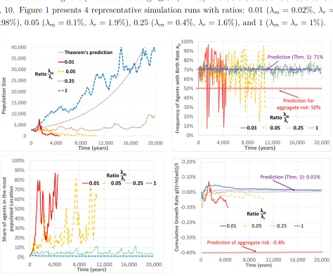
[image:12.612.71.545.171.564.2]local risk redrawing rate (while maintainingλm+λr= 2%): 0.01, 0.02, 0.05, 0.1, 0.25, 0.5, 1, 2, 4, 10. Figure 1 presents 4 representative simulation runs with ratios: 0.01 (λm = 0.02%, λr = 1.98%), 0.05 (λm = 0.1%, λr = 1.9%), 0.25 (λm = 0.4%, λr = 1.6%), and 1 (λm =λr= 1%).
Figure 1: Representative Simulation Runs for four Ratios of λm
λr
The top-left panel of Figure1shows the dynamics of the total population in each of the four simulation runs. The top-right panel shows how the frequency of agents that are endowed with a high local birth rate evolves. The bottom-left panel shows the percentage of agents that live in the most populated location (among the 300 locations). The bottom-right panel shows the
8
cumulative growth rate up to time t in each year (i.e., it shows g(t) = ln(wt(t))). The figure shows that when the ratio λm
λr is small (0.01 or 0.05), local risk has similar
properties to aggregate risk. The low rate of immigration implies that a couple of “successful” locations (which happen to have had a high local birth rate for a long time) concentrate most of the population. This causes the local risk, essentially, to be aggregate. The frequency of agents with a high local birth rate has large fluctuations, since a single change of the local birth rate of the most populated location has a large impact on this frequency. This is shown in the top-right panel. The cumulative growth rate (bottom-right panel) is initially positive, but after a couple of thousand years it becomes negative and starts converging to the negative growth predicted by aggregate risk, until the population becomes extinct (top-left panel).
By contrast, the figure shows that when the ratio λm
λr is 0.25 (resp., 1), then the predictions
of Theorem 1 become relatively (resp., very) accurate for the finite population. When the immigration rate is sufficiently high, a “successful” location spreads its offspring to many other locations, staving off extinction. The bottom-left panel shows that the frequency of agents living in the most populated location is at most 10% (resp., 2%). This implies that the share of agents with a high local birth rate has a relatively (resp., very) small fluctuations around Theorem1’s predicted value of about 71%, as can be seen in the top-right panel. The cumulative growth rate (bottom-right panel) converges to the positive value of 0.01%, as predicted in Theorem 1, as is shown in the top-left panel.
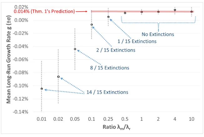
Figure2presents the mean long-run growth rate (and an interval of one standard deviation in each direction) obtained in the 15 simulation runs for each of the ten ratios of λm
λr. The
results show that when the ratio is 0.1 or smaller, then the mean growth rate is substantially less than its predicted value of 0.014%, and the population usually becomes extinct. The ratio of λm
λr = 0.25 is borderline: the mean growth rate (0.005%) is relatively close to what Theorem
1’s predicts, and the population becomes extinct only in a single simulation run. When the ratio of λm
λr is at least 0.5, Theorem 1 yields an excellent prediction: the mean growth rate is
very close to 0.014%, and the population does not become extinct in any simulation run.
6
Discussion
Age structure Recently, a different approach was applied byRobson & Samuelson(2019) to show that risk interdependence matters in a continuous-time setting (see also related results in
Figure 2: Mean Long-Run Growth Rate for each Ratio of λm
λr
The black points describe the mean growth rate of 15 simulation runs for each ratio of λm
λr . The
gray bars show intervals of one standard deviation on each side of the mean.
even without age structure, but still in a continuous-time setting. It would be interesting for future research to study the implications of local risk in age-structured populations.
Expected rate of reproduction Robatto & Szentes(2017, p. 418) summarize their paper by stating that when one regarding continuous environmental variations, natural selection would ensure that people’s “choices will be based only on the expected rate of reproduction.” We interpret the expected rate of reproduction simply as the expectation of a new draw of the birth rate. In a personal communication, Bal´azs Szentes suggested another interpretation of the expected rate of reproduction, according to which the expected rate of reproduction should be calculated as the average birth rate of all living agents at some distant time in the future. Under this interpretation, the expected rate of reproduction induced by local risk is higher than that induced by comparable aggregate or idiosyncratic risk. From this perspective, our paper then shows that, surprisingly, the relation between the two notions of expected birth rate is more complicated than the simple one-to-one relation in Robatto & Szentes’s model, whenever the birth rate has a local (or inherited) component.
which the species lives in a single large habitat. This result holds in a setup in which the birth rates are decreasing in the population’s density, and are deterministic. The present paper shows that connecting isolated small habitats with immigration increases the long-run growth rate. We adopt a complementary setup of the birth rate that does not depend on the population’s density, but does have a (local) stochastic component.
References
Burkey, Tormod Vaaland. 1999. Extinction in fragmented habitats predicted from stochas-tic birth–death processes with density dependence. Journal of Theoretical Biology, 199(4), 395–406.
Duffie, Darrell, & Sun, Yeneng. 2012. The exact law of large numbers for independent random matching. Journal of Economic Theory,147(3), 1105–1139.
Heller, Yuval. 2014. Overconfidence and diversification. American Economic Journal: Mi-croeconomics, 6(1), 134–153.
Lehmann, Laurent, & Balloux, François. 2007. Natural selection on fecundity variance in subdivided populations: Kin selection meets bet hedging. Genetics, 176(1), 361–377.
Lewontin, Richard C., & Cohen, Daniel. 1969. On population growth in a randomly varying environment. Proceedings of the National Academy of Sciences, 62(4), 1056–1060.
McNamara, John M. 1995. Implicit frequency dependence and kin selection in fluctuating environments. Evolutionary Ecology, 9(2), 185–203.
McNamara, John M., & Dall, Sasha R. X.2011. The evolution of unconditional strategies via the multiplier effect. Ecology Letters, 14(3), 237–243.
Robatto, Roberto, & Szentes, Balázs. 2017. On the biological foundation of risk prefe-rences. Journal of Economic Theory,172, 410–422.
Robson, Arthur J. 1996. A biological basis for expected and non-expected utility. Journal of Economic Theory, 68(2), 397–424.
Robson, Arthur J., & Samuelson, Larry. 2009. The evolution of time preference with aggregate uncertainty. American Economic Review, 99(5), 1925–1953.
Robson, Arthur J, & Samuelson, Larry. 2011. The evolutionary foundations of prefe-rences. Pages 221–310 of: Benhabib, Jess, Bisin, Alberto, & Jackson, Matthew
Robson, Arthur J., & Samuelson, Larry. 2019. Evolved attitudes to idiosyncratic and aggregate risk in age-structured populations. Journal of Eocnomic Theory, 181, 44–81.
Smith, James N. M., & Hellmann, Jessica J. 2002. Population persistence in fragmented landscapes. Trends in Ecology & Evolution, 17(9), 397–399.
A
Formal Proof
For each timet, letwh(t) be the number of agents with local birth ratexh at timet(henceforth,
xh-agents). Let αh(t) = wh(t)
w(t) be the share of xh-agents at time t. Let ¯b(t) the average birth
rate at timet: b¯(t) =P
kαk(t)·xk+µy+z(t). Letbh(t)be the average birth rate ofxh-agents
in time t: bh(t) =xh+µy+z(t). The mass of xh-agents at timet+ ∆tis given by (neglecting
terms of O(∆t)2 in all the following equations):
wh(t+ ∆t) =wh(t) + ∆t·((bh(t)−δ−λx)·wh(t) +w(t)·λx·q),
where∆t·bh(t)·wh(t)is the number of offspring that have been born in this brief period toxh
-agents,∆t·δ·wh(t)is the number ofxh-agents that have died in this brief period,∆t·λx·wh(t)
is the number of xh-agents that have changed their local birth rate in this brief period (either due to migration or due to their location having a new draw of its birth rate), and∆t·w(t)·λx·q
is the number of agents that have changed their local birth rate and obtained a realization of
xh for their new local risk in this brief period. The mass of agents at timet+ ∆t is given by
w(t+ ∆t) = w(t) + ∆t·¯b(t)−δ·w(t),
where ∆t·¯b(t)·w(t) is the mass of offspring born in this brief period, and ∆t·δ·w(t) is the mass of agents that died in this brief period. The share ofxh-agents at time t+ ∆t is given by:
αh(t+ ∆t) = wh(t+ ∆t)
w(t+ ∆t) =
αh(t) + ∆t·((bh(t)−δ−λx)αh(t) +λx·qx(xh))
1 + ∆t·b¯(t)−δ .
Multiplying by 1 + ∆t·b¯(t)−δ and rearranging the equation gives:
αh(t+ ∆t)−αh(t)
∆t = (bh(t)−δ−λx)·αh(t) +λx·q−
¯
b(t)−δ·αh(t+ ∆t),
dαh(t)
dt = (bh(t)−δ−λx)·αh(t) +λx·q−
¯
b(t)−δ·αh(t).
The expression on the right-hand side simplifies to
dαh(t)
dt = (1−αh(t))·αh(t)·(xh−xl) +λx·(q−αh(t)).
Letα∗
∈(q,1)be the unique positive number for which the right-hand side is equal to zero, where∆x:=xh −xl:
α∗
= ∆x−λx+
q
(∆x−λx)2+ 4·q·∆x·λx
2·∆x . (1)
It is immediate that:
dαh(t)
dt is
>0 αh(t)< α∗
= 0 αh(t) =α∗
<0 αh(t)> α∗
,
which implies global convergence to α∗
from any initial state, i.e., limt→∞αh(t) = α ∗
. This implies that the mean birth rate converges to
lim
t→∞
¯
b(t) = xl+α∗
·∆x+µy +z(t).
This, in turn, implies that the equivalent growth rate is given by:
g = lim
t→∞
logw(t)
t = limt→∞
¯
b(t)−δ=f(xl, xh, q, λx) +µy+µz−δ,
wheref(xl, xh, qx, λx)≡xl+α∗
·∆x. The limit of α∗
(λx) whenλx → ∞is given by:
lim
λx→∞α ∗
(λx) = lim
λx→∞
∆x−λx+λx·q1 + (2·q−1)·2· ∆x λx
2·∆x =
lim
λx→∞
∆x−λx+λx·1 + (2·q−1)· ∆x λx
2·∆x =
1 + (2·q−1) 2 =q,
and so
lim
λx→0
The limit of α∗
(λx) when λx →0 is given by:
limλx→0α ∗
(λx) = ∆x+ √
∆x2
2·∆x = 1,
and so
limλx→0f(xl, xh, qx, λx) = xh.
Next, we calculate the derivative of α∗
(λx) (1):
∂α∗
∂λx =
1 2·∆x
−
2·(∆x−λx) + 4·q·∆x
2·q(∆x−λx)2+ 4·q·∆x·λx −
1
.
We have to show that ∂α∗(λx)
∂λx is negative for any λx >0. This is true iff
q
(∆x−λx)2+ 4·q·∆x·λx >∆x·(2·q−1) +λx
After some algebra, this condition simplifies to
(∆x)2·1−(2·q−1)2>0,