Munich Personal RePEc Archive
New Hampshire Effect: Behavior in
Sequential and Simultaneous
Multi-Battle Contests
Mago, Shakun and Sheremeta, Roman
20 March 2018
Online at
https://mpra.ub.uni-muenchen.de/85337/
1
New Hampshire Effect:
Behavior in Sequential and Simultaneous Multi-Battle Contests
Shakun D. Mago a
Roman M. Sheremeta b,c,*
a Department of Economics, Robins School of Business, University of Richmond,
1 Gateway Road, Richmond, VA 23173, USA
b Weatherhead School of Management, Case Western Reserve University,
11119 Bellflower Road, Cleveland, OH 44106, USA
c Economic Science Institute, Chapman University
One University Drive, Orange, CA 92866
December 7, 2017
Abstract
Sequential multi-battle contests are predicted to induce lower expenditure than simultaneous contests. This prediction is a result of a “New Hampshire Effect” – a strategic advantage created by the winner of the first battle. Although our laboratory study provides evidence for the New Hampshire Effect, we find that sequential contests generate significantly higher (not lower) expenditure than simultaneous contests. This is mainly because in sequential contests, there is significant over-expenditure in all battles. We suggest sunk cost fallacy and utility of winning as two complementary explanations for this behavior and provide supporting evidence.
JEL Classifications: C72, C73, C91, D72
Keywords: election, sequential contests, simultaneous contests, experiments
* Corresponding author: Roman Sheremeta, [email protected]
2 1. Introduction
The nomination process for the U.S. presidential election consists of a series of nationwide
primary elections, beginning with the New Hampshire primary. The significance of this small New
England state became entrenched in the quadrennial election politics in 1952, when Estes Kefauver
defeated the incumbent President Harry Truman in the primary, leading Truman to abandon his
campaign. In 1988, all but one of George Bush’s Republican opponents withdrew soon after the
primary, and in 1992, number of Democratic Party candidates dwindled from five to two after the
primary (Busch and Mayer, 2004).1 Controlling for other factors, Mayer (2004) finds that a win in
the New Hampshire primary increases a candidate’s expected share of total primary votes by a
remarkable 26.6 percent.2
The perception that New Hampshire plays a pivotal and perhaps a disproportionately large
role in the presidential election (and thereby derives a wide array of political and economic benefits
from that position) led many states to move up the date of their primaries.3 ‘Frontloading’ is the
name given to a recent trend in the presidential nomination process in which more and more states
schedule their primaries near the beginning of the delegate selection process. Clustering of
primaries took a huge leap forward in 1988 with the formation of ‘Super Tuesday’ when 16 states
held their primaries on a single day in March. By 2008, 24 states held their primary on Super
1 Just as candidates who do poorly in the New Hampshire primary frequently drop out, the lesser-known, underfunded
candidates who do well in the primary suddenly become serious contenders to win the party nomination, garnering tremendous momentum both in terms of media coverage and campaign funding. In 1992, Bill Clinton, a little known governor of Arkansas did surprising well, and was labeled the “Comeback Kid” by the national media. In 2000, John McCain emerged as George Bush’s principal challenger only after an upset victory in New Hampshire, and a similar comeback was made by John Kerry in the 2004 primary.
2 In a multi-candidate race, even a second-place finish in New Hampshire primary increases a candidate’s final vote
by 17.2 percent (Mayer, 2004).
3 The total economic impact of 2000 primary on New Hampshire’s economy was estimated to be $264 million. The
3
Tuesday held in the first week of February. In 2004, James Roosevelt, co-chair of the Democratic
Party Rules Committee proclaimed: “We are moving towards a de facto national primary.”
For obvious reasons, with naturally-occurring data, it is difficult to examine the exact
impact of the two alternative electoral structures on both election outcomes and their economic
efficiency. For this reason, we use a controlled laboratory experiment to compare a sequential
contest, such as the current presidential primaries, to a simultaneous contest, as reflected in a
counterfactual national primary.4 Our theoretical framework is based on Klumpp and Polborn
(2006). In this political contest model, candidates have to win the majority of electoral districts in
order to obtain a prize – the party nomination. As in Tullock (1980) and Snyder (1989), candidates
can influence the probability of winning an electoral district by their choice of campaign
expenditure in that district. In case of a sequential contest, theory predicts that candidates should
spend disproportionately larger amounts in the earlier districts than in the later districts. This
difference in expenditure is attributed to the “New Hampshire Effect.” That is, the outcome of the
first election creates asymmetry between ex-ante symmetric candidates in terms of their incentive
to spend resources in the next district, which in turn, endogenously increases the probability that
the winner of the first district will win in subsequent districts and attain the final prize. For
example, in a sequential contest with three districts (battles), the winner of the first battle wins the
overall contest with probability of 0.875. Furthermore, the intense concentration of expenditure in
the initial battles entails that there is a 0.75 probability that the contest will end in only two battles.
In contrast, in case of a simultaneous contest, candidates are predicted to spend equal amounts of
4 Our experiment compares two extreme benchmarks: a completely sequential contest to a completely simultaneous
4
resources in all three battles. An important consequence of this temporal difference in contest
design is that the sequential contest is predicted to induce lower expenditure than the simultaneous
contest, which potentially could explain why political parties may choose the sequential electoral
structure of the primaries in order to minimize wasteful campaign expenditure.5
Our laboratory study of the three-battle contests provides evidence for the New Hampshire
Effect. We find that the strategic advantage created by the winner of the first battle makes it more
likely for him to win the entire contest. However, contrary to the theoretical predictions, we find
that sequential contests generate significantly higher (not lower) expenditure than simultaneous
contests. This is mainly because in sequential contests, there is significant over-expenditure in all
three battles. We suggest sunk cost fallacy and utility of winning as two complementary
explanations for this behavior and provide supporting evidence.
Analogies between our laboratory environment and the naturally-occurring political
contests are imperfect. Our design choices were made to facilitate analytical tractability and sharp
experimental investigation, and do not capture all the details of the real-world elections. For
instance, we assume that both contestants are symmetric and do not account for factors such as
name recognition, time of announcing candidacy, information aggregation, or the nature of
campaigns. We also ignore the carryover effect of winning (Schmitt et al., 2004), bandwagon effect
5 The contest model is complementary to the voters’ participation model (Morton and Williams, 1999; Battaglini et
5
(Callander, 2007) and the conditional promise of additional funding upon winning the primary
(Feigenbaum and Shelton, 2013). However, at least some of these factors do not detract from our
findings. For instance, theory predicts that the New Hampshire Effect holds even if players are
asymmetric in the sense that one is a better campaigner or has assured win in certain districts
(Klumpp and Polborn, 2006). In fact, the exogenous ex-ante asymmetry is further strengthened in
sequential contests by the endogenous ex-post asymmetry. Similarly, bandwagon theory and
carryover effect provide additional rationale for momentum to shift forward to earlier battles,
thereby reinforcing our results. Finally, sequential and simultaneous contests are not just restricted
to political contests, and can in fact be employed to study resource allocation problems in military
and systems defense (Clark and Konrad, 2007), research and development portfolio selection
(Clark and Konrad, 2008), and advertising (Friedman, 1958). By contrasting sequential and
simultaneous multi-battle contests in the simplest possible framework using laboratory data, which
is untainted from the various complicating factors that plague naturally-occurring data, we provide
a direct empirical test of the theoretical model of primary elections by Klumpp and Polborn (2006).
The rest of the paper is organized as follows. In Section 2, we provide a brief review of the
multi-battle contest literature, both theoretical and experimental. Section 3 presents our theoretical
framework and Section 4 describes the experimental design, procedures and hypotheses. Section
5 reports the results of our experiment and Section 6 concludes.
2. Literature Review
The theoretical literature on multi-battle contests originated with seminal work by
Fudenberg et al. (1983) and Snyder (1989).6 Fudenberg et al. (1983) model R&D competition as
6 One could also argue that the original formulation of a Colonel Blotto game by Borel (1921) is a starting point of
6
a sequential multi-battle contest, while Snyder (1989) models political campaigning as a
simultaneous multi-battle contest.7 For a comprehensive review of the theoretical literature on
multi-battle contests see Kovenock and Roberson (2012). Klumpp and Polborn (2006) directly
compare sequential and simultaneous multi-battle contests in a context of primary elections. They
show that the sequential contest creates a strategic advantage for the winner of the first battle, the
result they call a “New Hampshire Effect,” thus minimizing potentially wasteful expenditure in
future battles.
We conduct an experiment to test the predictions of the theoretical model by Klumpp and
Polborn (2006). While most of the existing experimental studies focus on single-battle contests,
recently there has been an increased interest in examining multi-battle contests (Avrahami and
Kareev, 2009; Arad and Rubinstein, 2012; Chowdhury et al., 2013; Mago and Sheremeta, 2017).
For a comprehensive review of this literature see Dechenaux et al. (2015). Experimental studies
on simultaneous multi-battle contests have examined how asymmetry in resources (Avrahami and
Kareev, 2009; Arad, 2012; Chowdhury et al., 2013), asymmetry in objectives (Kovenock et al.,
2010; Duffy and Matros, 2015; Holt et al., 2016; Montero et al., 2016), and asymmetry in battles
(Horta-Vallve and Llorente-Saguer, 2010; Avrahami et al., 2014) impact behavior in contests.
Experimental studies on sequential multi-battle contests have examined the impact of contest
structure (Deck and Sheremeta, 2012), carryover (Schmitt et al., 2004), fatigue (Ryvkin, 2011),
the length of the contest (Zizzo, 2002; Deck and Sheremeta, 2016), intermediate prizes and luck
(Mago et al., 2013; Gelder and Kovenock, 2017) on behavior in dynamic contests.8 Most of these
7 Building on these models, subsequent papers investigated the ramification of various factors such as the sequence
ordering of decisions, number of battles, asymmetry between players, effect of carryover, effect of uncertainty, the impact of discount factor and intermediate prizes (Harris and Vickers, 1985, 1987; Leininger, 1991; Baik and Lee, 2000; Szentes and Rosenthal, 2003; Roberson, 2006; Kvasov, 2007; Konrad and Kovenock, 2009).
8 Related to the studies on sequential multi-battle contests are the studies examining multi-battle elimination contests
7
studies find support for the comparative statics predictions (see the review by Dechenaux et al.,
2015), but often report significant over-expenditure of resources (also known as overbidding or
over-dissipation) relative to the Nash equilibrium prediction (see the reviews by Sheremeta, 2013,
2015).
Our study compares sequential and simultaneous multi-battle contests. Consistent with the
previous studies, we find significant over-expenditure relatively to the Nash equilibrium in both
contests. Our most surprising result is the reversal of the comparative statics prediction of Klumpp
and Polborn (2006) – we find that contrary to prediction, the sequential contest generates higher
expenditure than the simultaneous contest. This is surprising because, as mentioned above, almost
all contest experiments in the literature find strong support for the comparative statics predictions
even if the precise quantitative predictions are refuted. We suggest sunk cost fallacy and utility of
winning as possible explanations for this finding.
3. Theoretical Model
Consider two risk-neutral and equally-skilled players, 𝑋𝑋 and 𝑌𝑌, competing in a multi-battle
contest for an exogenously determined and commonly known prize v. There are 𝑛𝑛 battles in the
contest. Let 𝑥𝑥𝑖𝑖 and 𝑦𝑦𝑖𝑖 denote the amount of resource expenditure by players 𝑋𝑋 and 𝑌𝑌 in battle 𝑖𝑖.
Following Tullock (1980), the probabilities of winning battle 𝑖𝑖 by players 𝑋𝑋 and 𝑌𝑌 are defined by
a “lottery” contest success functions, such that a player’s probability of winning the battle depends
on his expenditure relative to the total expenditure:
𝑝𝑝𝑋𝑋𝑖𝑖(𝑥𝑥𝑖𝑖,𝑦𝑦𝑖𝑖) =𝑥𝑥𝑥𝑥𝑖𝑖
𝑖𝑖+𝑦𝑦𝑖𝑖 and 𝑝𝑝𝑌𝑌𝑖𝑖(𝑥𝑥𝑖𝑖,𝑦𝑦𝑖𝑖) =
𝑦𝑦𝑖𝑖
𝑥𝑥𝑖𝑖+𝑦𝑦𝑖𝑖 (1)
The player who wins a majority of the battles, i.e., at least (𝑛𝑛+1)/2 battles, wins the
8
𝑌𝑌) is equal to the value of the prize if he wins (zero otherwise) minus the total expenditure he has
spent during the contest:
𝜋𝜋𝑋𝑋 = �𝑣𝑣 − ∑ 𝑥𝑥𝑖𝑖 𝑛𝑛
𝑖𝑖=1 if 𝑋𝑋wins the contest
− ∑𝑛𝑛𝑖𝑖=1𝑥𝑥𝑖𝑖 otherwise (2)
The battles in the contest can proceed in two ways: sequentially or simultaneously. We
describe the theoretical predictions for both these cases with 𝑛𝑛= 3, although all the comparative
statics predictions hold for any 𝑛𝑛 ≥3 (Klumpp and Polborn, 2006). We chose 𝑛𝑛= 3 to simplify
the experimental environment and to facilitate greater subject comprehension.
3.1. Sequential Multi-Battle Contest
In the sequential multi-battle contest, players simultaneously choose expenditure levels 𝑥𝑥1
and 𝑦𝑦1 in battle 1. After determining the winner of battle 1, they move to battle 2 where they choose
expenditures 𝑥𝑥2 and 𝑦𝑦2. Players continue to compete until one player accumulates two victories.
The solution concept we consider is the subgame perfect Nash equilibrium. Using backward
induction, we begin our examination with the final and decisive battle 3. Note that if one of the
players has already won the previous two battles there is no need to compete in battle 3 and thus
expenditures are 𝑥𝑥3∗ =𝑦𝑦3∗ =0. However, if each player has won one of previous two battles then
the winner of the contest is determined by the result of battle 3. In such a case, player 𝑋𝑋’s expected
payoff (similarly for player 𝑌𝑌) is equal to the probability of player 𝑋𝑋 winning battle 3 𝑝𝑝𝑋𝑋3(𝑥𝑥3,𝑦𝑦3)
times the prize valuation 𝑣𝑣 minus cost of expenditure 𝑥𝑥3:
𝐸𝐸(𝜋𝜋𝑋𝑋3) =𝑝𝑝𝑋𝑋3(𝑥𝑥3,𝑦𝑦3)𝑣𝑣 − 𝑥𝑥3 =𝑥𝑥𝑥𝑥3
3+𝑦𝑦3𝑣𝑣 − 𝑥𝑥3 (3)
In the Nash equilibrium, battle 3 expenditures are 𝑥𝑥3∗ =𝑦𝑦3∗ =𝑣𝑣/4 and the expected payoffs
9
battle 1 and is leading the contest. Therefore, players are necessarily asymmetric, wherein player
𝑋𝑋 needs to win only one more battle to win the contest, while player 𝑌𝑌 needs to win two battles.
In this case, players 𝑋𝑋 and 𝑌𝑌 have the following expected payoffs:
𝐸𝐸(𝜋𝜋𝑋𝑋2) = 𝑥𝑥2
𝑥𝑥2+𝑦𝑦2𝑣𝑣+
𝑦𝑦2
𝑥𝑥2+𝑦𝑦2𝐸𝐸
∗(𝜋𝜋
3)− 𝑥𝑥2 and 𝐸𝐸(𝜋𝜋𝑌𝑌2) =𝑥𝑥2𝑦𝑦+𝑦𝑦2 2𝐸𝐸∗(𝜋𝜋3)− 𝑦𝑦2 (4)
Note that player 𝑋𝑋’s value of winning battle 2 is higher than that of player 𝑌𝑌. Consequently,
in battle 2 player 𝑋𝑋 chooses higher expenditure than player 𝑌𝑌, and is more likely to win the overall
contest. Klumpp and Polborn (2006) call this outcome the “New Hampshire Effect” – the outcome
of battle 1 has an asymmetric effect on expenditures of ex-ante symmetric players. In the Nash
equilibrium, battle 2 expenditures are 𝑥𝑥2∗ =9𝑣𝑣/64 and 𝑦𝑦2∗ =3𝑣𝑣/64 and the expected payoffs are
𝐸𝐸∗(𝜋𝜋
𝑋𝑋2) =43𝑣𝑣/64 and 𝐸𝐸∗(𝜋𝜋𝑌𝑌2) =𝑣𝑣/64. Finally, going back to battle 1, the players are symmetric
again. Both players need to accumulate two battle victories to win the contest. In this case, player
𝑋𝑋 (similarly, player 𝑌𝑌) maximizes the following expected payoff:
𝐸𝐸(𝜋𝜋𝑋𝑋1) = 𝑥𝑥1
𝑥𝑥1+𝑦𝑦1𝐸𝐸
∗(𝜋𝜋
𝑋𝑋2) +𝑥𝑥𝑦𝑦1
1+𝑦𝑦1𝐸𝐸
∗(𝜋𝜋
𝑌𝑌2) − 𝑥𝑥1 (5)
In the Nash equilibrium of this subgame, battle 1 expenditures are 𝑥𝑥1∗ =𝑦𝑦1∗ =21𝑣𝑣/128 and
the expected payoffs are 𝐸𝐸∗(𝜋𝜋𝑋𝑋1) =𝐸𝐸∗(𝜋𝜋𝑌𝑌1) =𝐸𝐸∗(𝜋𝜋1) =23𝑣𝑣/128. Both players have the same
expenditure profile because they have the same value for winning battle 1. Aggregating across all
three battles, the expected equilibrium expenditure by each player is 41𝑣𝑣/128.
3.2. Simultaneous Multi-Battle Contest
In the simultaneous multi-battle contest, players simultaneously choose expenditure levels
𝑥𝑥𝑖𝑖 and 𝑦𝑦𝑖𝑖 for all three battles 𝑖𝑖= 1, 2, 3. Then, the winner of each individual battle is determined
10
that each battle of the multi-battle contest is an ‘independent’ lottery contest. Therefore, player 𝑋𝑋
(similarly, player 𝑌𝑌) maximizes the following expected payoff:
𝐸𝐸(𝜋𝜋𝑋𝑋) =��3 3� �
𝑥𝑥 𝑥𝑥+𝑦𝑦�
3
+ �3 2� �
𝑥𝑥 𝑥𝑥+𝑦𝑦�
2
�𝑥𝑥+𝑦𝑦𝑦𝑦 �� 𝑣𝑣 −3𝑥𝑥=�� 𝑥𝑥
𝑥𝑥+𝑦𝑦� 3
+ 3𝑥𝑥2𝑦𝑦
(𝑥𝑥+𝑦𝑦)3� 𝑣𝑣 −3𝑥𝑥 (6)
In the unique Nash equilibrium, both players make the same expenditure in all battles, i.e.,
𝑥𝑥𝑖𝑖∗= 𝑦𝑦
𝑖𝑖∗ =𝑣𝑣/8 for all 𝑖𝑖.9 Aggregating across all three battles, the expected equilibrium
expenditure by each player is 48𝑣𝑣/128.
4. Experimental Environment
4.1. Experimental Design and Hypotheses
We employ two treatments: sequential and simultaneous. In the sequential treatment two
players compete in a sequential multi-battle contest, while in the simultaneous treatment two
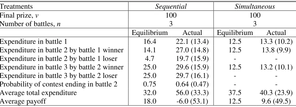
players compete in a simultaneous multi-battle contest. Table 1 summarizes the equilibrium
predictions in both treatments for 𝑣𝑣= 100 and 𝑛𝑛 =3. These predictions motivate the following
three hypotheses:
Hypothesis 1: Total expected expenditure in the sequential contest is lower compared to
the simultaneous contest.
The expected total expenditure by a player in the sequential contest is 32.4, and in the
simultaneous contest is 37.5.
Hypothesis 2: In the sequential contest, the winner of battle 1 is more likely to win battle
2 and the overall contest.
11
In the sequential contest, the outcome of battle 1 creates asymmetry between ex-ante
symmetric players. This asymmetry endogenously triggers differing expenditure levels in the
subsequent battles and generates momentum for the winner of battle 1, also known as the “New
Hampshire Effect.” Since it is less likely for the loser of battle 1 to win the contest, the absolute
level of expenditure falls sharply after the outcome of battle 1 is known. In battle 2, the winner of
battle 1 exerts three times more expenditure than the loser. As a result, sequential contest ends
after two battles with probability 0.75, and the winner of battle 1 wins the overall contest with
probability 0.875.
Hypothesis 3: In the simultaneous contest, expenditures are uniformly distributed across
all three battles.
Since all three battles are identical in the simultaneous contest, both players make the same
expenditure of 12.5 in each battle. This is in sharp contrast to the sequential contest where
expenditures are predicted to be more intensely concentrated in the first battle.10
4.2. Experimental Procedures
A total of 144 subjects participated in 12 sessions (12 subjects per session). All subjects
were undergraduate students at Chapman University and inexperienced in this decision-making
environment.11 No one participated in more than one session. The experimental sessions were run
using computer software z-Tree (Fischbacher, 2007). Throughout the session, no communication
between subjects was permitted, and all choices and information were transmitted via computer
10 In the sequential contest, the total expected expenditure by both players in battle 1 is 32.8; in battle 2 is 18.8; and
since battle 3 is likely to occur with probability 0.25, the unconditional expected expenditure in battle 3 is 25.
11 48% of our subjects identified as males and 52% as females. The average age of the participants was 19.63 and
12
terminals. At the beginning of each session, subjects received an initial endowment of $20 to cover
any potential losses.
Each experimental session corresponded to 20 periods of play in one of the two treatments.
Thus, 6 sessions featured the sequential treatment and 6 sessions featured the simultaneous
treatment, generating a total of 1440 observations for each treatment (6 sessions × 12 subjects ×
20 periods). Subjects were given the instructions, available in the Appendix A, at the beginning of
the experiment, and these were read aloud by the experimenter. Before the start of the experiment,
subjects completed a computerized multiple choice quiz to verify their understanding of the
instructions.12 The experiment started only after all subjects completed the quiz and explanations
were provided for any incorrect answers. In every period, subjects were randomly and
anonymously placed into 6 groups with 2 players in each group. To keep the terminology neutral,
in the instructions we describe the task as one of making bids in boxes and the player who wins 2
boxes gets the prize of 100 experimental francs. We gave detailed explanations and numerical
examples for the mechanisms underlying the contest structures, and how winners are determined
in each battle (i.e., the lottery rule). Subjects were informed that increasing their bid would increase
their chance of winning; and that regardless of who wins the prize, all subjects would have to pay
their bids. In the simultaneous treatment subjects were asked to make bids in three battles
simultaneously. They were not allowed to bid more than 100 francs in any battle and money spent
on bidding was subtracted from the initial endowment of $20.13 After subjects submitted their bids,
12 Subjects also made 15 choices in simple lotteries, similar to Holt and Laury (2002), at the beginning of the
experiment. These were used to elicit their risk aversion preferences, and subjects were paid for one randomly selected choice. We did not find any interesting patterns or correlations between risk attitudes and behavior in contests. So, we omit any discussion from the article.
13 100 francs is substantially higher than the highest possible equilibrium bid, but we decided not to constrain
13
the computer displayed own bids, opponent’s bids, the winner of each battle, the overall winner
and own final payoff. In the sequential treatment subjects made their bidding decision sequentially,
either in two or three rounds (with bids not exceeding 100 francs in any round). At the end of each
round, the computer displayed own bid, opponent’s bid, and the winner of the battle in that round.
The period ended when one of the subjects in the group won two rounds. At the end of each period,
subjects were randomly re-grouped to form a new two-person group.
At the end of the experiment, 2 out of 20 periods were randomly selected for payment.14
The sum of the earnings for these 2 periods was exchanged at rate of 25 experimental francs = US
$1. On average, the experimental sessions lasted for about 60 minutes, and subjects earned $21
which was paid anonymously and in cash.
5. Results
5.1. General Results
Table 2 presents the mean expenditure and payoff in both sequential and simultaneous
contests. The average total expenditure is 56.0 in the sequential contest and 40.3 in the
simultaneous contest. While the observed expenditure in the simultaneous contest is not
significantly different from the equilibrium predictions (40.3 versus 37.5; Wilcoxon signed-rank
test, p-value = 0.24, n = 6), the observed expenditure in the sequential contest is significantly
higher than predicted (56.0 versus 32.0; Wilcoxon signed-rank test, p-value = 0.02, n = 6). We
also corroborate the conclusions from these conservative nonparametric tests by estimating
multivariate panel regression models.15
14 We chose to select only 2 periods for payment in order to avoid intra-experimental income effects (McKee, 1989).
In addition, subjects were paid for their lottery choice from the risk elicitation procedure.
15 We have checked the robustness of these results by estimating a mixed-effects panel model for each treatment (see
14
Over-expenditure in contests is a commonly observed phenomenon (Sheremeta, 2013,
2015; Dechenaux et al., 2015), and therefore, the result that total expenditure in the simultaneous
contest conforms to the theoretical predictions may seem surprising. However, as we discuss later,
instead of following the equilibrium strategy of allocating their resources to all three battles,
subjects use the incomplete coverage strategy by focusing their expenditure on just two battles.
Expenditure in these two battles average at 16.3, which exceeds the equilibrium prediction of 12.5.
Therefore, one could speculate that we would also observe over-expenditure in the simultaneous
multi-battle contest if subjects did not use a non-equilibrium strategy of incomplete coverage of
battles. We discuss this in more detail in Section 5.3.
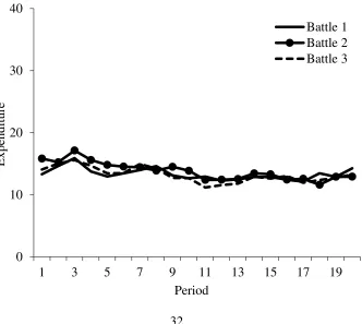
The experiment lasted for 20 periods and it is relevant to examine how expenditure evolves
over the length of the experiment. Figures 1 and 2 show that expenditure decreases over time in
the sequential and simultaneous contests. In the sequential contest, the average total expenditure
drops from 62.9 in the first half of the experiment to 49.0 in the second half. In the simultaneous
contest, it drops from 42.9 in the first half to 37.8 in the second half. Panel regressions confirm
that these declines are statistically significant (p-values < 0.01).16 Overall, our result that
over-expenditure decreases with repetition in the direction of equilibrium play is consistent with
previous experimental findings on single-battle contests (Davis and Reilly, 1998; Sheremeta and
Zhang, 2010; Price and Sheremeta, 2011, 2015; Chowdhury et al., 2014; Mago et al., 2016).
dependent variable in the regression is the total expenditure and the independent variables are a constant and a period trend. The model included a mixed-effects error structure with a 3-way nested model (observations nested within a session and then within a subject) to account for the multiple decisions made by each subject and random re-matching within a session. A standard Wald test, conducted on estimates of regression models, shows that expenditure in the sequential contest is significantly higher than predicted (p-value < 0.01) and for the simultaneous contest it is not different from the prediction (p-value = 0.60). Hypothesis testing with a few clusters (sessions) can result in over-rejection of the null hypothesis. To address this concern, we also conducted regressions based on Cameron et al. (2008) wild cluster approach. The results remain the same – expenditure in the sequential contest is significantly higher than predicted and for the simultaneous contest it is not different from the prediction.
15
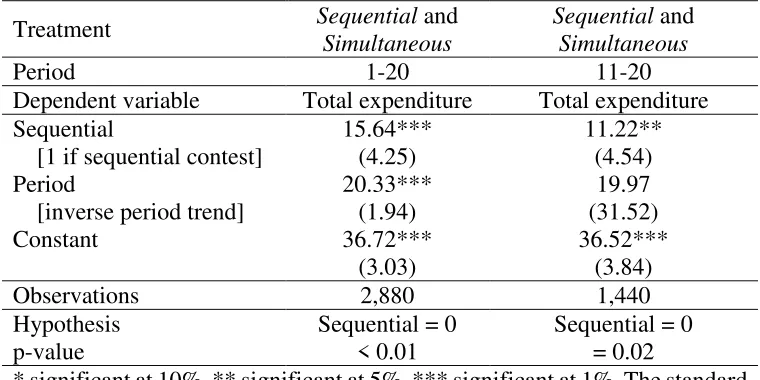
A comparison across the two treatments informs our Hypothesis 1 that the average total
expenditure is lower in the sequential contest relative to the simultaneous contest (32.0 versus
37.5). Contrary to this prediction, however, we find that the average total expenditure in the
sequential contest is higher than in the simultaneous contest (56.0 versus 40.3; Wilcoxon
rank-sum test, p-value = 0.01, n1 = 6, n2 = 6). This is also true when we restrict our attention only to the
second half of the experiment (49.0 versus 37.8; Wilcoxon rank-sum test, p-value = 0.05, n1 = 6,
n2 = 6).17 It is important to emphasize that the magnitude of the difference between the two
treatments is quite substantial in size. The sequential contest generates almost 40% higher
expenditure than the simultaneous contest, instead of the predicted 20% lower expenditure. As a
result of this over-expenditure, the observed average payoff in the sequential contest is negative
and lower than prediction (-6.0 versus 18.0). On the other hand, the average payoff in the
simultaneous contest is positive and very close to prediction (9.6 versus 12.5).
Finding 1: Average total expenditure is significantly higher in the sequential contest than
in the simultaneous contest (evidence against Hypothesis 1).
Next, we take a closer look at the individual battle behavior in both sequential and
simultaneous contests.
5.2. Sequential Contests
One of our central predictions is that the sequential contest generates the New Hampshire
Effect, so that the winner of battle 1 is more likely to win battle 2 and the overall contest
(Hypothesis 2). For our parameters, the winner of battle 1 is predicted to win the overall contest
17 Mixed-effects panel regressions collaborate the results of the non-parametric statistical tests (see Table B2 in
16
with probability 0.875. In the experiment, we find that the winner of battle 1 wins the overall
contest with probability 0.83, and this qualitative result persist through all 20 periods of the
experiment, as evident in Figure 3. It is important to note that a best of three coin‐toss model would
also generate a probability of 0.75 that the winner of battle 1 wins the overall contest. However,
both a binomial test of proportions and a conservative non-parametric test indicate that the
observed probability of winning is significantly higher than the prediction from the coin‐toss
model (0.83 versus 0.75; test of proportions, p-value < 0.01; Wilcoxon signed-rank test, p-value =
0.02, n = 6). Thus, consistent with the New Hampshire Effect, we find that the winner of the battle
1 is more likely to win the overall contest.
Another prediction emerging from the New Hampshire Effect entails that winning battle 1
creates asymmetry, leading the winner of battle 1 to spend more in battle 2 than the loser of battle
1. More specifically, for our parameters, theory predicts that the winner of battle 1 should spend
14.1 in battle 2 and the loser of battle 1 should spend 4.7 in battle 2 (see Table 1). Consistent with
this prediction, we find that the average expenditure in battle 2 by battle 1 winner is significantly
higher than the average expenditure in battle 2 by battle 1 loser (27.0 versus 19.7; Wilcoxon
rank-sum test, p-value = 0.02, n1 = 6, n2 = 6).18
Finding 2: In the sequential contest, the winner of battle 1 wins battle 2 and the overall
contest more often than the loser of battle 1 (evidence for Hypothesis 2).
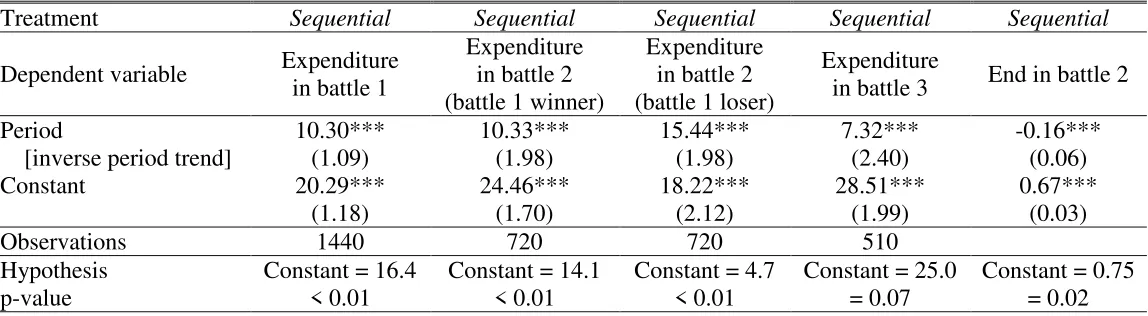
Although we find significant support for the New Hampshire Effect, we also find important
deviations from the theory. First, relative to the theoretical benchmarks, we find over-expenditure
in all battles. The expenditure in battle 1 is significantly higher than predicted (22.1 versus 16.4;
18 A mixed-effects panel regression collaborates the results of the non-parametric statistical tests (see Table B3 in
17
Wilcoxon signed-rank test, p-value = 0.02, n = 6). The same is true for the expenditure in battle 2
by battle 1 winner (27.0 versus 14.1; Wilcoxon signed-rank test, p-value = 0.02, n = 6), the
expenditure in battle 2 by battle 1 loser (19.7 versus 4.7; Wilcoxon signed-rank test, p-value =
0.02, n = 6), and the expenditure in battle 3 (29.6 versus 25.0; Wilcoxon signed-rank test, p-value
= 0.04, n = 6).19 Our observation of over-expenditure in all three battles is inconsistent with the
theoretical predictions of the model, but it can explain why the sequential contests generate much
a higher total expenditure than the simultaneous contests (Finding 1).
Second, contrary to the predictions, expenditure in battle 2 is greater than in battle 1.
Specifically, the theory predicts that the expenditure of battle 1 winner should decrease from 16.4
in battle 1 to 14.1 in battle 2. Instead, the data show that battle 1 winners do not decrease their
battle 2 expenditure (25.1 versus 27.0; Wilcoxon signed-rank test, p-value = 0.24, n = 6), with
84% of expenditure in battle 2 being higher than the equilibrium prediction of 14.1, as shown in
Figure 4. Similarly, contrary to the predicted decrease in expenditure from 16.4 in battle 1 to 4.7
in battle 2, battle 1 losers also do not decrease their battle 2 expenditure (19.1 versus 19.7;
Wilcoxon signed-rank test, p-value = 0.91, n = 6), with 81% of expenditure in battle 2 being higher
than the equilibrium prediction of 4.7, as shown in Figure 4.
Finally, aggressive play by both players explains why the sequential contest lasts longer
than expected. Contrary to the theoretical prediction that the sequential contest should end in battle
2 with probability 0.75, we find that on average the contest ends in battle 2 with probability 0.65.20
However, there is some evidence of learning since the likelihood of battle 2 being the decisive one
is increasing with the repetition of the experiment (see Figure 3). For example, in the first half of
19 The non-parametric statistical tests are also corroborated by mixed-effect panel regressions (see Table B4 in
Appendix B). Regressions based on Cameron et al. (2008) wild cluster approach produce similar results.
18
the experiment 60% of the contests conclude after two battles, and this proportion increased to
68% in the second half.
Finding 3: In the sequential contest, over-expenditure is observed in all three battles.
Contrary to the theoretical prediction, both battle 1 winner and battle 1 loser do not decrease their
expenditure in battle 2 relative to battle 1. As a result, the probability of contest ending in two
battles is lower than predicted.
Significant over-expenditure is consistent with previous findings of contest experiments
(Dechenaux et al., 2015; Sheremeta, 2017) and various explanations have been offered in the
literature (Sheremeta, 2013, 2015).21 We will focus on two explanations: sunk cost and utility of
winning. These factors are naturally linked to the multi-stage sequential contests and can explain
the observed over-expenditure in these contests; but in addition they also offer an insight into the
difference across sequential and simultaneous contests.
5.2.1. Sunk Cost Fallacy
The payoff maximization problem underlying the multi-battle sequential contest
equilibrium regards the expenditure in previous battles as sunk cost, and therefore ignores them.
However, the sequential nature of the contest can create an irrational regard for sunk cost, or in
other words, subjects can fall prey to the sunk cost fallacy (Staw, 1976). Evidence from various
behavioral studies find that cognitive dissonance can induce people who have sunk resources into
an unprofitable activity to irrationally revise their beliefs about the profitability of an additional
expenditure, in order to avoid the unpleasant acknowledgment that they made a mistake (Friedman
21 Explanations for over-expenditure in single-battle contests include non-monetary utility of winning (Sheremeta,
19
et al., 2007; Baliga and Ely, 2011; Just and Wansink, 2011; Augenblick, 2016). In our experiment,
subjects who get to battle 2 have already made some expenditure in battle 1. If the sunk cost
hypothesis is true, it should entail that subjects who spend more resources in battle 1 are also more
likely to spend more in battle 2 – to increase their chance of winning the prize and recoup some of
their expenditure. Indeed, we find a positive and significant relationship between the expenditure
in battle 2 and battle 1 (p-value < 0.01).22 However, this positive relationship also could arise
because of the presence of a subset or “type” of subjects who tend to spend more in all battles of
the sequential contest. Therefore, to provide direct empirical evidence for the sunk cost hypothesis
in our experimental environment, we collected additional data from a modified version of the
sequential contest.
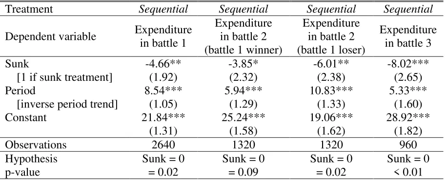
We ran 5 sessions of a modified version of the sequential contest at Chapman University.
The 60 subjects who participated in these additional sessions faced rules that were essentially the
same as in the original sequential contest, with the only difference that the subjects did not make
any expenditure in battle 1 and the winner of that battle was determined randomly by a computer.
This feature allows us to see how subjects behave in battle 2 without prior sunk cost expenditure.
Our hypothesis is that if subjects fall prey to sunk cost fallacy then expenditure in the latter battles
of the modified contests would be less than in the original sequential contest. Indeed, we find
strong support for our hypothesis (and thereby, the sunk cost explanation). In battle 2, expenditure
in the modified sequential contest is 25% lower than in the original sequential contest (18.7 versus
23.3; Wilcoxon rank-sum test, p-value = 0.06, n1 = 5, n2 = 6). This is also true when we separate
our sample by battle 1 winner (22.1 versus 27.0; Wilcoxon rank-sum test, p-value = 0.06, n1 = 5,
n2 = 6) and battle 1 loser (15.2 versus 19.7; Wilcoxon rank-sum test, p-value = 0.04, n1 = 5, n2 =
20
6).23 However, relative to the theoretical predictions, the expenditure in battle 2 is still significantly
higher for battle 1 winner (22.1 versus 14.1; Wilcoxon signed-rank test, p-value = 0.04, n = 5) and
for battle 1 loser (15.2 versus 4.7; Wilcoxon signed-rank test, p-value = 0.04, n = 5).
Extending this sunk cost argument to battle 3, it follows that since subjects make lower
expenditure in battle 2 we should also observe lower expenditure in battle 3 of the modified
sequential contest. In support of this hypothesis, we find that battle 3 expenditure in the modified
sequential contest is 36% lower than in the original sequential contest (21.5 versus 29.7; Wilcoxon
rank-sum test, p-value = 0.01, n1 = 5, n2 = 6).24 Moreover, in the modified sequential contest, the
expenditure in battle 3 is not statistically different from the theoretical predictions (21.5 versus
25.0; Wilcoxon signed-rank test, p-value = 0.13, n = 5).
Therefore, we find direct empirical evidence supporting the sunk cost explanation for
significant over-expenditure in the sequential multi-battle contest. This irrational regard for sunk
cost can also explain why the sequential contests generate higher total expenditure than the
simultaneous contests (Finding 1). Although the number of battles is identical in both simultaneous
and sequential contest, the temporal sequencing of the sequential contest results in a sunk cost
fallacy while this effect is absent in the simultaneous contest.
5.2.2. Utility of Winning
Cox et al. (1988) were among the first to suggest the utility of winning as an explanation
for overbidding in auctions, and Goeree et al. (2002) used an empirical strategy to identify the
23 The non-parametric statistical tests are also collaborated by mixed-effect panel regressions (see Table B5 in
Appendix B). In estimating these regressions, we used a battle 2 expenditure as the dependent variable and a treatment dummy-variable, a period trend, and a constant as the independent variables. Regressions based on Cameron et al. (2008) wild cluster approach produce similar results.
21
utility of winning. In a contest framework, Sheremeta (2010b) proposed a method of directly
measuring the utility of winning in an incentive compatible way. Since then, numerous
experimental studies have employed non-monetary utility of winning as an explanation for
over-expenditure in contests (Sheremeta, 2013, 2015; Cason et al., 2011, 2012; Price and Sheremeta,
2011, 2015; Mago et al., 2016).
We employ the non-monetary utility of winning to explain some patterns in our data that
cannot be explained by the sunk cost fallacy. Specifically, in the sequential contest, we find that
the reduced probability of the contest ending in battle 2 and the resulting over-expenditure is
largely driven by the increased expenditure in battle 2, by both battle 1 winner and battle 1 loser
(Finding 3). Since this increased expenditure is not grounded in standard equilibrium explanation
and may not be completely accounted for by the sunk cost fallacy, we postulate that subjects may
derive additional non-monetary utility from winning itself. 25
Based on the assumption that subjects care only about their monetary prize, standard
equilibrium theory predicts that battle 1 loser will suffer from a dramatic decrease in his
continuation value for the next battle, and accordingly spend less in battle 2; given this, the winner
of battle 1 will also reduce his expenditure in battle 2. However, if we incorporate winning as a
component in the subject’s utility function, the decline in continuation value is not so dramatic for
either players. Following similar theoretical models presented in Parco et al. (2005), Amaldoss
and Rapoport (2009), and Sheremeta (2010b, 2013), suppose the non-monetary utility takes an
additive form, i.e., in addition to the value of the prize 𝑣𝑣, individuals also have a non-monetary
25 As evidenced in the prior discussion, sunk cost fallacy cannot explain all the deviations from the theory. Even in
22
utility of winning 𝑤𝑤, where 0≤ 𝑤𝑤 ≤ 𝑣𝑣. Then instead of (3), the updated expected payoff in battle
3 becomes:
𝐸𝐸′(𝜋𝜋𝑋𝑋3) = 𝑥𝑥3
𝑥𝑥3+𝑦𝑦3(𝑣𝑣+𝑤𝑤)− 𝑥𝑥3, (7)
Similarly, instead of (4), the updated expected payoffs in battle 2 become:
𝐸𝐸′(𝜋𝜋𝑋𝑋2) = 𝑥𝑥2
𝑥𝑥2+𝑦𝑦2(𝑣𝑣+𝑤𝑤) +
𝑦𝑦2
𝑥𝑥2+𝑦𝑦2𝐸𝐸
′∗(𝜋𝜋
3)− 𝑥𝑥2 and 𝐸𝐸′(𝜋𝜋𝑌𝑌2) =𝑥𝑥2𝑦𝑦+𝑦𝑦2 2(𝐸𝐸′∗(𝜋𝜋3) +𝑤𝑤)− 𝑦𝑦2 (8)
Finally, instead of (5), the updated payoff in battle 1 becomes:
𝐸𝐸′(𝜋𝜋𝑋𝑋1) = 𝑥𝑥1
𝑥𝑥1+𝑦𝑦1(𝐸𝐸
′∗(𝜋𝜋
𝑋𝑋2) +𝑤𝑤) +𝑥𝑥1𝑦𝑦+𝑦𝑦1 1𝐸𝐸′∗(𝜋𝜋𝑌𝑌2) − 𝑥𝑥1. (9)
Although we cannot obtain a closed form solution analytically, we can solve this model
numerically. Figure 5 shows expenditures in the sequential contest in all three battles as a function
of the utility of winning 𝑤𝑤, for 𝑤𝑤 ∈ [0,100]. It is clear that the utility of winning gives incentive
to both players to engage in higher spending. Specifically, upon accounting for 𝑤𝑤, both winner
and loser of battle 1 make higher than predicted expenditures in battle 2 for 𝑤𝑤 ∈(0,100]; and
despite this over-dissipation, the expenditure in battle 2 by battle 1 winner is higher than by battle
1 loser for 𝑤𝑤 ∈ [0,100). This predicted pattern of expenditure is consistent with our Finding 2.
Furthermore, the utility of winning provides an equilibrium explanation for why the loser
of battle 1 does not decrease his/her expenditure in battle 2 as much as predicted (Finding 3). From
Figure 5 it is evident that as 𝑤𝑤 increases, the gap in expenditure in battle 2 by winner and loser of
battle 1, and the corresponding New Hampshire Effect, decreases. In fact, when utility of winning
is equal to prize of the contest (𝑣𝑣 =𝑤𝑤 = 100) the equilibrium expenditure of the winner is same
as that of the loser.
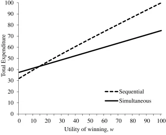
Utility of winning may also provide insight into why expenditure is significantly higher in
sequential contests compared to simultaneous contests (Finding 1). Both Parco et al. (2005) and
23
Although the number of battles is identical in both simultaneous and sequential contest, in the
sequential contest subjects can receive non-monetary utility of winning up to two times (when
each battle winner is announced) while in the simultaneous contest such utility is received only
once (when the overall winner is announced). Figure 6 shows total expenditure in sequential and
simultaneous contests as a function of the utility of winning 𝑤𝑤, for 𝑤𝑤 ∈[0,100]. It is evident that
the sequential contest generates higher total expenditure than the simultaneous contest for 𝑤𝑤 ∈
[15,100] (i.e., higher than 15% of the prize value 𝑣𝑣= 100). The lower bound for 𝑤𝑤 is fairly
conservative, given the results of Sheremeta (2010a, 2010b) and Price and Sheremeta (2010,
2015), where 𝑤𝑤 is estimated to be around 50% of the prize value.
5.3. Simultaneous Contests
For the simultaneous contest, theory predicts that subjects allocate expenditure equally
across all the three battles (Hypothesis 3). Our data reveals that although the average expenditure
in all three battles is close to the predicted level of 12.5 (Table 2), none of the subjects who
participated in the simultaneous contest employ a uniform expenditure strategy. Most subjects vary
their expenditure between battles, with the difference from the mean expenditure across all three
battles averaging at a steep 12.1. Figure 7 displays the average difference from the mean
expenditure across all three battles in a given period. A lower magnitude of dispersion implies a
more uniform expenditure strategy and obviously, in equilibrium, the magnitude of dispersion
should be zero. We find that although there is some evidence that the dispersion of expenditure
across the three battles decreases in the first five periods of the experiment; on the whole, the
average difference in expenditure between battles remains positive and significant over the entire
24
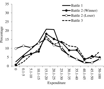
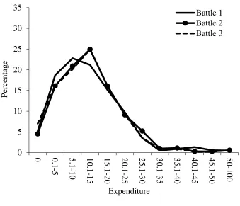
Figure 8 displays the distribution of expenditure within each battle over all 20 periods of
the simultaneous contest. Two things stand out. First, despite the large variance, the overall
distribution of expenditure is remarkably similar in the three battles indicating no preferential bias
between battles.26 Second, subjects’ expenditures are distributed over the entire strategy space,
which is clearly inconsistent with play at a unique pure strategy Nash equilibrium. While a large
majority of the expenditure is centered close to the equilibrium prediction of 12.5, there is also
substantial variation in expenditure.
Finding 4: Subjects in the simultaneous contest do not employ a uniform expenditure
strategy. There is substantial dispersion in expenditure both between-battles in a given period and
within-battles over time.
This dispersion in expenditure (both between and within battles) alludes to a strategy akin
to “guerilla warfare.” To win the overall contest, a player needs to win a minimum of two battles.
She does not derive any additional utility from winning all three battles. This suggests that players
can randomly select and focus their expenditure on just two battles. We find that the average
minimum expenditure in a battle is 7.7, almost half the prediction of 12.5. Indeed, 24% of time,
expenditure in one of the battles is less than or equal to 1. Similarly, expenditure in the remaining
two battles averages at 16.3, and exceeds the equilibrium prediction more 62% of the time.
Although contrary to the theoretical prediction, focusing on the minimal set of battles which are
sufficient for victory has an intuitive appeal and such behavior has been observed in other
multi-battle contest experiments (see the review by Sheremeta, 2017).27
26 That is, there is no allocation bias such as that observed in Colonel Blotto games (Chowdhury et al., 2013), where
players who read and write from left to right horizontally in their native language tend to allocate greater expenditure to the battles on the left.
27 It is important to emphasize, however, that the “guerilla warfare” strategy is not an equilibrium strategy. In fact, in
25 6. Conclusion
In this study we use a laboratory experiment to compare sequential and simultaneous
contests, where candidates have to win the majority of battles in order to obtain a prize. Candidates
influence the probability of winning a battle by their choice of expenditure in that battle. We find
that, contrary to prediction, sequential contests generate significantly higher expenditure than
simultaneous contests. This is mainly because in sequential contests, there is significant
over-expenditure in all three battles. We suggest sunk cost fallacy and utility of winning as two
complementary explanations for this behavior and provide supporting evidence.
Our findings have implications both for policy makers and social scientists. In particular,
the finding that sequential contests induce higher expenditure (and thus more inefficiency) than
simultaneous contests is both interesting and puzzling. Previous theoretical and empirical research
on sequential and simultaneous voting provides mixed evidence in favor of sequential system
(Morton and Williams, 1999, 2000; Klumpp and Polborn, 2006). Battaglini et al. (2007), for
example, find that a sequential voting rule is more efficient but less equitable than simultaneous
voting in some information environments. We show that, on the contrary, simultaneous contest
dominates sequential contest because it generates substantially lower expenditure. Thus, we
provide evidence that attempts such as ‘Frontloading’ and ‘Super Tuesday’ to make presidential
nomination process more like the simultaneous contest may indeed lead to a more efficient and
significantly less costly electoral process. Furthermore, our result that sunk costs result in higher
expenditure in the sequential costs may have important implications for the organizational
structure of the primaries. The choice of New Hampshire, which represent 0.4 percent of the U.S.
26
as possible. Similarly, utility of winning may be one of the explanations why candidates with later
finishes continue to seek the nomination.
Our theoretical construct is a prototype model of a strategic multi-dimensional resource
allocation game (Kovenock and Roberson, 2012). Although our experimental design is built
around the theoretical model of Klumpp and Polborn (2006), who compare sequential and
simultaneous multi-battle contests in the context of primary elections, our design can also be used
to analyze problems in various fields such as military and systems defense (Hausken, 2008),
advertising resource allocation (Friedman, 1958), and research and development portfolio
selection (Clark and Konrad, 2008).
Our experimental design considers the simplest setting of two symmetric players in a
three-battle contest. While our experimental framework captures some of the most salient features of
sequential and simultaneous contests, we have set aside empirically relevant issues, such as
candidate strength differences, state‐specific advantages, and endogenous donations, which limits
the external validity of our results. Extending our design to account for these issues remains a
promising avenue for future research. For instance, given the observed deviations from predictions,
it would be interesting to study how behavior evolves in case of more battles and/or asymmetric
27 References
Altmann, S., Falk, A. & Wibral, M. (2012). Promotions and incentives: The case of multistage elimination tournaments. Journal of Labor Economics, 30, 149-174.
Amegashie, J.A., Cadsby, C.B., & Song, Y. (2007). Competitive burnout: Theory and experimental evidence. Games and Economic Behavior, 59, 213-239.
Arad, A. & Rubinstein, A. (2012). Multi-dimensional iterative reasoning in action: The case of the Colonel Blotto game. Journal of Economic Behavior and Organization, 84, 571-585.
Arad, A. (2012). The Tennis Coach problem: A game-theoretic and experimental study. The B.E. Journal of Theoretical Economics, 12, 10.
Augenblick, N. (2016). The sunk-cost fallacy in penny auctions. Review of Economic Studies, 83, 58-86.
Avrahami, J., & Kareev, Y. (2009). Do the weak stand a chance? Distribution of resources in a competitive environment. Cognitive Science, 33, 940-950.
Baik, K. & Lee, S. (2000).Two-stage rent-seeking contests with carryovers. Public Choice, 103, 285-296.
Baliga, S., & Ely, J.C. (2011). Mnemonomics: The sunk cost fallacy as a memory kludge. American Economic Journal: Microeconomics, 3, 35-67.
Battaglini, M., Morton, R.B., & Palfrey, T.R. (2007). Efficiency, equity and timing of voting mechanisms. American Political Science Review, 101, 409-424.
Borel, E. (1921). La theorie du jeu les equations integrales a noyau symetrique. Comptes Rendus del Academie. 173, 1304-1308; English translation by Savage, L. (1953). The theory of play and integral equations with skew symmetric kernels. Econometrica, 21, 97-100.
Busch, A., & Mayer, W. (2004). The front-loading problem. In: Mayer, W. (Eds.), The making of the presidential candidate. Rowman and Littlefied Publishers, Inc, USA, 83-132.
Callander, S. (2007). Bandwagons and momentum in sequential voting. Review of Economic Studies, 74, 653-684
Cameron, A.C., Gelbach, J.B., & Miller, D.L. (2008). Bootstrap-based improvements for inference with clustered errors. Review of Economics and Statistics, 90, 414-427.
Cason, T.N., Masters, W.A. & Sheremeta, R.M. (2011). Winner-take-all and proportional-prize contests: Theory and experimental results. Working Paper.
Cason, T.N., Sheremeta, R.M., & Zhang, J. (2012). Communication and efficiency in competitive coordination games. Games and Economic Behavior, 76, 26-43.
Chowdhury, S.M., Kovenock, D. & Sheremeta, R.M. (2013). An experimental investigation of Colonel Blotto games. Economic Theory, 52, 833-861.
Chowdhury, S.M., Sheremeta, R.M., Turocy, T.L. (2014). Overbidding and overspreading in rent-seeking experiments: Cost structure and prize allocation rules. Games and Economic Behavior. 87, 224-238.
Clark, D.J., & Konrad, K.A. (2007). Asymmetric conflict weakest link against best shot. Journal of Conflict Resolution, 51, 457-469.
Clark, D.J., & Konrad, K.A. (2008). Fragmented property rights and incentives for R&D. Management Science, 54, 969-981.
Cox, J.C., Smith, V.L., & Walker, J.M. (1988). Theory and individual behavior of first-price auctions. Journal of Risk and Uncertainty, 1, 61-99.
28
Dechenaux, E., Kovenock, D. & Sheremeta, R.M. (2015). A Survey of experimental research on contests, all-pay auctions and tournaments. Experimental Economics, 18, 609-669.
Deck, C. & Sheremeta, R.M. (2012). Fight or flight? Defending against sequential attacks in the Game of Siege. Journal of Conflict Resolution, 56, 1069-1088.
Deck, C. & Sheremeta, R.M. (2016). Tug-of-war in the laboratory. Working Paper.
Duffy, J., & Matros, A. (2015). Stochastic asymmetric Blotto games: Some new results. Economics Letters, 134, 4-8.
Feigenbaum, J.J., & Shelton, C.A. (2013). The vicious cycle: Fundraising and perceived viability in US presidential primaries. Quarterly Journal of Political Science, 8, 1-40.
Fischbacher, U. (2007). z-Tree: Zurich toolbox for ready-made economic experiments. Experimental Economics, 10, 171-178.
Friedman, D., Pommerenke, K., Lukose, R., Milam, G. & Huberman, B. (2007) Searching for the sunk cost fallacy. Experimental Economics, 10, 79-104.
Friedman, L. (1958). Game-theory models in the allocation of advertising expenditure. Operations Research, 6, 699-709.
Fudenberg, D., Gilbert, R., Stiglitz, J., & Tirole, J. (1983). Preemption, leapfrogging and competition in patent races. European Economic Review, 22, 3-31.
Gelder, A., & Kovenock, D. (2017). Dynamic behavior and player types in majoritarian multi-battle contests. Games and Economic Behavior, 104, 444-455.
Goeree, J.K., Holt, C.A., & Palfrey, T.R. (2002). Quantal response equilibrium and overbidding in private-value auctions. Journal of Economic Theory, 104, 247-272.
Harris, C., & Vickers, J. (1985). Perfect equilibrium in a model of a race. Review of Economic Studies, 52, 193-209.
Harris, C., & Vickers, J. (1987). Racing with uncertainty. Review of Economic Studies, 54, 1-21. Hausken, K. (2008). Strategic defense and attack for series and parallel reliability systems.
European Journal of Operational Research, 186, 856-881.
Höchtl, W., Kerschbamer, R., Stracke, R. & Sunde, U. (2015). Incentives vs. selection in promotion tournaments: Can a designer kill two birds with one stone? Managerial and Decision Economics, 36, 275-285.
Holt, C.A. & Laury, S.K. (2002). Risk aversion and incentive effects. American Economic Review, 92, 1644-1655.
Holt, C.A., Kydd, A., Razzolini, L., & Sheremeta, R. (2016). The paradox of misaligned profiling theory and experimental evidence. Journal of Conflict Resolution, 60, 482-500.
Hortala-Vallve, R. & Llorente-Saguer, A. (2010). A simple mechanism for resolving conflict. Games and Economic Behavior, 70, 375-391.
Just, D.R., & Wansink, B. (2011). The flat-rate pricing paradox: Conflicting effects of “all-you-can-eat” buffet pricing. Review of Economics and Statistics, 93, 193-200.
Klumpp, T., & Polborn, M.K. (2006). Primaries and the New Hampshire effect. Journal of Public Economics, 90, 1073-1114.
Konrad, K.A., & Kovenock, D. (2009). Multi-battle contests. Games Economic Behavior, 66, 256-274.
Kovenock, D. & Roberson, B (2012). Conflicts with multiple battlefields. In Garfinkel, M.R., Skaperdas, S. (Eds.), Oxford Handbook of the Economics of Peace and Conflict. New York: Oxford University Press, pp. 503-531.
29
Kvasov, D. (2007). Contests with limited resources. Journal of Economic Theory, 136, 738-748. Leininger, W. (1991). Patent competition, rent dissipation, and the persistence of monopoly: the
role of research budgets. Journal of Economic Theory, 53, 146-172.
Mago, S.D. & Sheremeta, R.M. (2017). Multi-battle contests: An experimental study. Southern Economic Journal, forthcoming.
Mago, S.D., Savikhin, A.C. & Sheremeta, R.M. (2015). Facing your opponents: Social identification and information feedback in contests. Journal of Conflict Resolution, 60, 459-481.
Mago, S.D., Sheremeta, R.M. & Yates, A. (2013). Best-of-three contest experiments: Strategic versus psychological momentum. International Journal of Industrial Organization, 31, 287-296.
Mayer, W. (2004). The basic dynamics of contemporary nomination process. In: Mayer, W. (Eds.), The making of the presidential candidate. Rowman and Littlefied Publishers, Inc, USA, 83-132.
McKee, M. (1989). Intra-experimental income effects and risk aversion. Economic Letters, 30, 109-115.
Montero, M., Possajennikov, A., Sefton, M., & Turocy, T.L. (2016). Majoritarian Blotto contests with asymmetric battlefields: An experiment on Apex games. Economic Theory, 61, 55-89. Morton, R.B., & Williams, K.C. (1999). Information asymmetries and simultaneous versus
sequential voting. American Political Science Review, 93, 51-67.
Morton, R.B., & Williams, K.C. (2000). Learning by voting: Sequential choices in presidential primaries and other elections. Ann Arbor, MI: University of Michigan Press.
Parco J., Rapoport A., & Amaldoss W. (2005). Two-stage contests with budget constraints: An experimental study. Journal of Mathematical Psychology, 49, 320-338.
Price, C.R. & Sheremeta, R.M. (2011). Endowment effects in contests. Economics Letters, 111, 217-219.
Price, C.R. & Sheremeta, R.M. (2015). Endowment origin, demographic effects and individual preferences in contests. Journal of Economics and Management Strategy, 24, 597-619.
Roberson, B. (2006). The Colonel Blotto game. Economic Theory, 29, 1-24.
Ryvkin, D. (2011). Fatigue in dynamic tournaments. Journal of Economics and Management Strategy, 20, 1011-1041.
Schmitt, P., Shupp, R. Swope, K., & Cadigan, J. (2004). Multi-period rent-seeking contests with carryover: Theory and experimental evidence. Economics of Governance, 10, 247-259. Sheremeta, R.M. (2010a). Expenditures and information disclosure in two-stage political contests.
Journal of Conflict Resolution, 54, 771-798.
Sheremeta, R.M. (2010b). Experimental comparison of multi-stage and one-stage contests. Games and Economic Behavior, 68, 731-747.
Sheremeta, R.M. (2011). Contest design: An experimental investigation. Economic Inquiry, 49, 573-590.
Sheremeta, R.M. (2013). Overbidding and heterogeneous behavior in contest experiments. Journal of Economic Surveys, 27, 491-514.
Sheremeta, R.M. (2015). Behavioral dimensions of contests. In Congleton, R.D., Hillman, A.L., (Eds.), Companion to the Political Economy of Rent Seeking, London: Edward Elgar, pp. 150-164.
30
Sheremeta, R.M. (2017). Experimental research on contests. Working Paper.
Sheremeta, R.M., & Zhang, J. (2010). Can groups solve the problem of over-bidding in contests? Social Choice and Welfare, 35, 175-197.
Shupp, R., Sheremeta, R.M., Schmidt, D., & Walker, J. (2013). Resource allocation contests: Experimental evidence. Journal of Economic Psychology, 39, 257-267.
Snyder, J. (1989). Election goals and the allocation of campaign resources. Econometrica, 57, 630-660.
Staw, B.M. (1976). Knee-deep in the big muddy: A study of escalating commitment to a chosen course of action. Organizational Behavior and Human Performance, 16, 27-44.
Szentes, B., & Rosenthal, R.W. (2003). Beyond chopsticks: Symmetric equilibria in majority auction games. Games and Economic Behavior, 45, 278-295.
Tullock, G. (1980). Efficient rent seeking. In James M. Buchanan, Robert D. Tollison, Gordon Tullock, (Eds.), Toward a theory of the rent-seeking society. College Station, TX: Texas A&M University Press, pp. 97-112.
31
Table 1: Equilibrium Predictions in Sequential and Simultaneous Contests
Treatments Sequential Simultaneous
Final prize, v 100 100
Number of battles, n 3 3
Equilibrium Equilibrium
Expenditure in battle 1 16.4 12.5
Expenditure in battle 2 by battle 1 winner 14.1 12.5
Expenditure in battle 2 by battle 1 loser 4.7 -
Expenditure in battle 3 25.0 12.5
Probability of contest ending in battle 2 0.75 -
Expected total expenditure 32.0 37.5
Expected payoff 18.0 12.5
Table 2: Average Statistics
Treatments Sequential Simultaneous
Final prize, v 100 100
Number of battles, n 3 3
Equilibrium Actual Equilibrium Actual
Expenditure in battle 1 16.4 22.1 (13.4) 12.5 13.3 (10.2)
Expenditure in battle 2 by battle 1 winner 14.1 27.0 (14.8) 12.5 13.8 (9.9)
Expenditure in battle 2 by battle 1 loser 4.7 19.7 (15.9) - -
Expenditure in battle 3 by battle 2 winner 25.0 29.6 (15.9) 12.5 13.2 (10.1)
Expenditure in battle 3 by battle 2 loser 25.0 29.7 (16.1) - -
Probability of contest ending in battle 2 0.75 0.64 (0.47) - -
Average total expenditure 32.0 56.0 (33.3) 37.5 40.3 (23.9)
Average payoff 18.0 -6.0 (53.1) 12.5 9.6 (49.5)
[image:32.612.71.547.336.509.2]32
Figure 1: Average Expenditure over 20 Periods in the Sequential Contest
Figure 2: Average Expenditure over 20 Periods in the Simultaneous Contest 0
10 20 30 40 50
1 3 5 7 9 11 13 15 17 19
E
x
pe
ndi
tur
e
Period
Battle 1
Battle 2 (Winner) Battle 2 (Loser) Battle 3
0 10 20 30 40
1 3 5 7 9 11 13 15 17 19
E
x
pe
ndi
tur
e
Period
[image:33.612.144.476.441.738.2]33
Figure 3: Probability of Ending and Winning the Sequential Contest
Figure 4: Distribution of Expenditure in the Sequential Contest 0 0.2 0.4 0.6 0.8 1
1 3 5 7 9 11 13 15 17 19
P ro b ab ility Period
End in Battle 2
Win by a Battle 1 Winner
0 5 10 15 20 25 30 35 0 0.1-5 5.1-10 10.1-15 15.1-20 20.1-25 25.1-30 30.1-35 35.1-40 40.1-45 45.1-50 50-100 P er cen tag e Expenditure Battle 1
[image:34.612.140.476.439.726.2]34
Figure 5: Expenditure in the Sequential Contest as a Function of the Utility of Winning
Figure 6: Total Expenditure in Sequential and Simultaneous Contests as a Function of the Utility of Winning
0 10 20 30 40 50
0 10 20 30 40 50 60 70 80 90 100
E
x
pe
ndi
tur
e
Utility of winning, w
Battle 1
Battle 2 (Winner) Battle 2 (Loser) Battle 3
0 10 20 30 40 50 60 70 80 90 100
0 10 20 30 40 50 60 70 80 90 100
T
ot
al
E
x
pe
ndi
tur
e
Utility of winning, w
[image:35.612.136.473.445.719.2]35
Figure 7: Average Difference from the Mean Expenditure across Three Battles in the
Simultaneous Contest
Figure 8: Distribution of Expenditure in the Simultaneous Contest 0
5 10 15 20
1 3 5 7 9 11 13 15 17 19
[image:36.612.138.477.438.729.2]