Interpretable Semantic Vectors from a Joint Model of Brain and Text Based Meaning

Interpretable Semantic Vectors from a Joint Model of Brain- and

Text-Based Meaning

Alona Fyshe1_{, Partha P. Talukdar}1_{, Brian Murphy}2_{, Tom M. Mitchell}1 1_{Machine Learning Department, Carnegie Mellon University} 2_{School of Electronics, Electrical Engineering and Computer Science}

Queen’s University Belfast

[afyshe,partha.talukdar,tom.mitchell]@cs.cmu.edu [email protected]

Abstract

Vector space models (VSMs) represent word meanings as points in a high dimen-sional space. VSMs are typically created using a large text corpora, and so repre-sent word semantics as observed in text. We present a new algorithm (JNNSE) that can incorporate a measure of semantics not previously used to create VSMs: brain activation data recorded while people read words. The resulting model takes advan-tage of the complementary strengths and weaknesses of corpus and brain activation data to give a more complete representa-tion of semantics. Evaluarepresenta-tions show that the model 1) matches a behavioral mea-sure of semantics more closely, 2) can be used to predict corpus data for unseen words and 3) has predictive power that generalizes across brain imaging technolo-gies and across subjects. We believe that the model is thus a more faithful represen-tation of mental vocabularies.

1 Introduction

Vector Space Models (VSMs) represent lexical meaning by assigning each word a point in high di-mensional space. Beyond their use in NLP appli-cations, they are of interest to cognitive scientists as an objective and data-driven method to discover word meanings (Landauer and Dumais, 1997).

Typically, VSMs are created by collecting word usage statistics from large amounts of text data and applying some dimensionality reduction technique like Singular Value Decomposition (SVD). The basic assumption is that semantics drives a per-son’s language production behavior, and as a result co-occurrence patterns in written text indirectly encode word meaning. The raw co-occurrence statistics are unwieldy, but in the compressed

VSM the distance between any two words is con-ceived to represent their mutual semantic similar-ity (Sahlgren, 2006; Turney and Pantel, 2010), as perceived and judged by speakers. This space then reflects the “semantic ground truth” of shared lex-ical meanings in a language community’s vocab-ulary. However corpus-based VSMs have been criticized as being noisy or incomplete representa-tions of meaning (Glenberg and Robertson, 2000). For example, multiple word senses collide in the same vector, and noise from mis-parsed sentences or spam documents can interfere with the final se-mantic representation.

When a person is reading or writing, the se-mantic content of each word will be necessarily activated in the mind, and so in patterns of ac-tivity over individual neurons. In principle then, brain activity could replace corpus data as input to a VSM, and contemporary imaging techniques allow us to attempt this. Functional Magnetic Res-onance Imaging (fMRI) and Magnetoencephalog-raphy (MEG) are two brain activation recording technologies that measure neuronal activation in aggregate, and have been shown to have a pre-dictive relationship with models of word mean-ing (Mitchell et al., 2008; Palatucci et al., 2009; Sudre et al., 2012; Murphy et al., 2012b).1

If brain activation data encodes semantics, we theorized that including brain data in a model of semantics could result in a model more consistent with semantic ground truth. However, the inclu-sion of brain data will only improve a text-based model if brain data contains semantic information not readily available in the corpus. In addition, if a semantic test involves another subject’s brain activation data, performance can improve only if the additional semantic information is consistent across brains. Of course, brains differ in shape, size and in connectivity, so additional information encoded in one brain might not translate to

an-1_{For more details on fMRI and MEG, see Section 4.2}

other. Furthermore, different brain imaging tech-nologies measure very different correlates of neu-ronal activity. Due to these differences, it is possi-ble that one subject’s brain activation data cannot improve a model’s performance on another sub-ject’s brain data, or for brain data collected using a different recording technology. Indeed, inter-subject models of brain activation is an open re-search area (Conroy et al., 2013), as is learning the relationship between recording technologies (En-gell et al., 2012; Hall et al., 2013). Brain data can also be corrupted by many types of noise (e.g. recording room interference, movement artifacts), another possible hindrance to the use of brain data in VSMs.

VSMs are interesting from both engineering and scientific standpoints. In this work we fo-cus on the scientific question: Can the inclusion of brain data improve semantic representations learned from corpus data? What can we learn from such a model? From an engineering perspective, brain activation data will likely never replace text data. Brain activation recordings are both expen-sive and time consuming to collect, whereas tex-tual data is vast and much of it is free to download. However, from a scientific perspective, combining text and brain data could lead to more consistent semantic models, in turn leading to a better un-derstanding of semantics and semantic modeling generally.

In this paper, we leverage both kinds of data to build a hybrid VSM using a new matrix factor-ization method (JNNSE). Our hypothesis is that the noise of brain and corpus derived statistics will be largely orthogonal, and so the two data sources will have complementary strengths as in-put to VSMs. If this hypothesis is correct, we should find that the resulting VSM is more suc-cessful in modeling word semantics as encoded in human judgements, as well as separate corpus and brain data that was not used in the derivation of the model. We will show that our method:

1. creates a VSM that is more correlated to an independent measure of word semantics. 2. produces word vectors that are more

pre-dictable from the brain activity of different people, even when brain data is collected with a different recording technology. 3. predicts corpus representations of withheld

words more accurately than a model that does not combine data sources.

4. directly maps semantic concepts onto the brain by jointly learning neural representa-tions.

Together, these results suggest that corpus and brain activation data measure semantics in com-patible and complimentary ways. Our results are evidence that a joint model of brain- and text-based semantics may be closer to seman-tic ground truth than text-only models. Our findings also indicate that there is additional se-mantic information available in brain activation data that is not present in corpus data, and that there are elements of semantics currently lack-ing in text-based VSMs. We have made avail-able the top performing VSMs created with brain

and text data (http://www.cs.cmu.edu/

˜afyshe/papers/acl2014/).

In the following sections we will review NNSE, and our extension, JNNSE. We will describe the data used and the experiments to support our posi-tion that brain data is a valuable source of semantic information that compliments text data.

2 Non-Negative Sparse Embedding

Non-Negative Sparse Embedding (NNSE) (Mur-phy et al., 2012a) is an algorithm that produces a latent representation using matrix factorization. Standard NNSE begins with a matrixX ∈ Rw×c

made of c corpus statistics for w words. NNSE solves the following objective function:

argmin

A,D w X

i=1

_{Xi,:−Ai,:×D}2_+λA 1

(1) subject to:Di,:DTi,:≤1,∀1≤i≤` (2)

Ai,j ≥0, 1≤i≤w, 1≤j ≤` (3)

The solution will find a matrixA ∈ Rw×` _{that is}

sparse, non-negative, and represents word seman-tics in an`-dimensional latent space. D ∈ R`×c

gives the encoding of corpus statistics in the la-tent space. Together, they factor the original cor-pus statistics matrix X in a way that minimizes the reconstruction error. TheL1constraint

The sparse and non-negative representation in A produces a more interpretable semantic space, where interpretability is quantified with a behav-ioral task (Chang et al., 2009; Murphy et al., 2012a). To illustrate the interpretability of NNSE, we describe a word by selecting the word’s top scoring dimensions, and selecting the top scoring words in those dimensions. For example, the word chair has the following top scoring dimensions:

1. chairs, seating, couches; 2. mattress, futon, mattresses; 3. supervisor, coordinator, advisor.

These dimensions cover two of the distinct mean-ings of the word chair (furniture and person of power).

NNSE’s sparsity constraint dictates that each word can have a non-zero score in only a few di-mensions, which aligns well to previous feature elicitation experiments in psychology. In feature elicitation, participants are asked to name the char-acteristics (features) of an object. The number of characteristics named is usually small (McRae et al., 2005), which supports the requirement of spar-sity in the learned latent space.

3 Joint Non-Negative Sparse Embedding

We extend NNSEs to incorporate an additional source of data for a subset of the words in X, and call the approach Joint Non-Negative Sparse Embeddings (JNNSEs). The JNNSE algorithm is general enough to incorporate any new infor-mation about the a word w, but for this study we will focus on brain activation recordings of a human subject reading single words. We will incorporate either fMRI or MEG data, and call the resulting models JNNSE(fMRI+Text) and JNNSE(MEG+Text) and refer to them generally as JNNSE(Brain+Text). For clarity, from here on, we will refer to NNSE as NNSE(Text), or NNSE(Brain) depending on the single source of input data used.

Let us order the rows of the corpus data X so that the first1. . . w0_{rows have both corpus}

statis-tics and brain activation recordings. Each brain activation recording is a row in the brain data ma-trixY ∈Rw0_×v

wherevis the number of features derived from the recording. For MEG recordings, v=sensors×time points= 306×150. For fMRI v=grey-matter voxels='20,000depending on the brain anatomy of each individual subject. The

new objective function is:

argmin

A,D(c)_,D(b) w X

i=1

_{Xi,:−Ai,:×D}(c)2₊

w0

X

i=1

_{Yi,:−Ai,:×D}(b)2_+λA 1

(4) subject to: D(_i,c_:)D_i,(c_:)T ≤1,∀1≤i≤` (5) D<sub>i,</sub>(b<sub>:</sub>)D<sub>i,</sub>(b<sub>:</sub>)T ≤1,∀1≤i≤` (6) Ai,j ≥0, 1≤i≤w, 1≤j≤`

(7) We have introduced an additional constraint on the rows 1. . . w0_{, requiring that some of the learned}

representations inAalso reconstruct the brain ac-tivation recordings (Y) through representations in D(b) _{∈ R}`×v_{. Let us useA}0 _{to refer to the}

brain-constrained rows of A. Words that are close in “brain space” must have similar representations in A0_{, which can further percolate to affect the}

rep-resentations of other words in Avia closeness in “corpus space”.

With A or D fixed, the objective function for NNSE(Text) and JNNSE(Brain+Text) is convex. However, we are solving forAandD, so the prob-lem is non-convex. To solve for this objective, we use the online algorithm of Section 3 from Mairal et al. (Mairal et al., 2010). This algorithm is guaranteed to converge, and in practice we found that JNNSE(Brain+Text) converged as quickly as NNSE(Text) for the same`. We used the SPAMS package2 _{to solve, and set λ = 0.025. This}

al-gorithm was a very easy extension to NNSE(Text) and required very little additional tuning.

We also consider learning shared representa-tions in the case where dataX andY contain the effects of knowndisjoint features. For example, when a person reads a word, the recorded brain activation data Y will contain the physiological response to viewing the stimulus, which is unre-lated to the semantics of the word. These sig-nals can be attributed to, for example, the num-ber of letters in the word and the numnum-ber of white pixels on the screen (Sudre et al., 2012). To ac-count for such effects in the data, we augment A0 _{with a set of n fixed, manually defined}

fea-tures (e.g. word length) to create A0

percept ∈

Rw×(`+n)<sub>.D</sub>(b)<sub>∈R</sub>(`+n)×v_{is used withA}0

to reconstruct the brain data Y. More gener-ally, one could instead allocate a certain num-ber of latent features specific to X or Y, both of which could be learned, as explored in some re-lated work (Gupta et al., 2013). We use 11

per-ceptualfeatures that characterize the non-semantic

features of the word stimulus (for a list, see sup-plementary material athttp://www.cs.cmu. edu/˜afyshe/papers/acl2014/).

The JNNSE algorithm is advantageous in that it can handle partially paired data. That is, the algorithm does not require that every row in X also have a row in Y. Fully paired data is a re-quirement of many other approaches (White et al., 2012; Jia and Darrell, 2010). Our approach al-lows us to leverage the semantic information in corpus data even for words without brain activa-tion recordings.

JNNSE(Brain+Text) does not require brain data to be mapped to a common average brain, which is often the case when one wants to generalize be-tween human subjects. Such mappings can blur and distort data, making it less useful for subse-quent prediction steps. We avoid these mappings, and instead use the fact that similar words elicit similar brain activation within a subject. In the JNNSE algorithm, it is this closeness in “brain space” that guides the creation of the latent space A. Leveraging intra-subject distance measures to study inter-subject encodings has been studied previously (Kriegeskorte et al., 2008a; Raizada and Connolly, 2012), and has even been used across species (humans and primates) (Kriegesko-rte et al., 2008b).

Though we restrict ourselves to using one sub-ject per JNNSE(Brain+Text) model, the JNNSE algorithm could easily be extended to include data from multiple brain imaging experiments by adding a new squared loss term for additional brain data.

3.1 Related Work

Perhaps the most well known related approach to joining data sources is Canonical Correlation Analysis (CCA) (Hotelling, 1936), which has been applied to brain activation data in the past (Rus-tandi et al., 2009). CCA seeks two linear trans-formations that maximally correlate two data sets in the transformed form. CCA requires that the data sources be paired (all rows in the corpus data must have a corresponding brain data), as corre-lation between points is integral to the objective.

To apply CCA to our data we would need to dis-card the vast majority of our corpus data, and use only the 60 rows of X with corresponding rows in Y. While CCA holds the input data fixed and maximally correlates the transformed form, we hold the transformed form fixed and seek a solu-tion that maximally correlates the reconstrucsolu-tion (AD(c)_orA0_D(b)_{) with the data (XandY}

respec-tively). This shift in error compensation is what allows our data to be only partially paired. While a Bayesian formulation of CCA can handle miss-ing data, our model has missmiss-ing data for>97%of the fullw×(v+c)brain and corpus data matrix. To our knowledge, this extreme amount of missing data has not been explored with Bayesian CCA.

One could also use a topic model style formula-tion to represent this semantic representaformula-tion task. Supervised topic models (Blei and McAuliffe, 2007) use a latent topic to generate two observed outputs: words in a document and a categorical la-bel for the document. The same idea could be ap-plied here: the latent semantic representation gen-erates the observed brain activity and corpus statis-tics. Generative and discriminative models both have their own strengths and weaknesses, gener-ative models being particularly strong when data sources are limited (Ng and Jordan, 2002). Our task is an interesting blend of data-limited and data-rich problem scenarios.

In the past, various pieces of additional informa-tion have been incorporated into semantic models. For example, models with behavioral data (Sil-berer and Lapata, 2012) and models with visual information (Bruni et al., 2011; Silberer et al., 2013) have both shown to improve semantic rep-resentations. Other works have correlated VSMs built with text or images with brain activation data (Murphy et al., 2012b; Anderson et al., 2013). To our knowledge, this work is the first to integrate brain activation data into the construction of the VSM.

4 Data

4.1 Corpus Data

The corpus statistics used here are the download-able vectors from Fyshe et al. (2013)3_{. They}

are compiled from a 16 billion word subset of ClueWeb09 (Callan and Hoy, 2009) and contain two types of corpus features: dependency and doc-ument features, found to be complimentary for

3_{http://www.cs.cmu.edu/˜afyshe/papers/}

most tasks. Dependency statistics were derived by dependency parsing the corpus and compil-ing counts for all dependencies incident on the word. Document statistics are word-document co-occurrence counts. Count thresholding was applied to reduce noise, and positive pointwise-mutual-information (PPMI) (Church and Hanks, 1990) was applied to the counts. SVD was ap-plied to the document and dependency statistics and the top 1000 dimensions of each type were retained. We selected the rows corresponding to noun-tagged words (approx. 17000 words).

4.2 Brain Activation Data

We have MEG and fMRI data at our disposal. MEG measures the magnetic field caused by many thousands of neurons firing together, and has good time resolution (1000 Hz) but poor spatial reso-lution. fMRI measures the change in blood oxy-genation that results from differential neural ac-tivity, and has good spatial resolution but poor time resolution (0.5-1 Hz). We have fMRI data and MEG data for 18 subjects (9 in each imaging modality) viewing 60 concrete nouns (Mitchell et al., 2008; Sudre et al., 2012). The 60 words span 12 word categories (animals, buildings, tools, in-sects, body parts, furniture, building parts, uten-sils, vehicles, objects, clothing, food). Each of the 60 words was presented with a line drawing, so word ambiguity is not an issue. For both record-ing modalities, all trials for a particular word were averaged together to create one training instance per word, with 60 training instances in all for each subject and imaging modality. More preprocess-ing details appear in the supplementary material.

5 Experimental Results

Here we explore several variations of JNNSE and NNSE formulations. For a comparison of the models used, see Table 1.

5.1 Correlation to Behavioral Data

To test if our joint model of Brain+Text is closer to semantic ground truth we compared the latent representationAlearned via JNNSE(Brain+Text) or NNSE(Text) to an independent behavioral mea-sure of semantics. We collected behavioral data for the 60 nouns in the form of answers to 218 semantic questions. Answers were gathered with Mechanical Turk. The full list of questions ap-pear in the supplementary material. Some exam-ple questions are:“Is it alive?”, and “Can it bend?”. Mechanical Turk users were asked to respond to

each question for each word on a scale of 1-5. At least 3 respondents answered each question and the median score was used. This gives us a se-mantic representation of each of the 60 words in a 218-dimensional behavioral space. Because we required answers to each of the questions for all words, we do not have the problems of sparsity that exist for feature production norms from other studies (McRae et al., 2005). In addition, our swers are ratings, rather than binary yes/no an-swers.

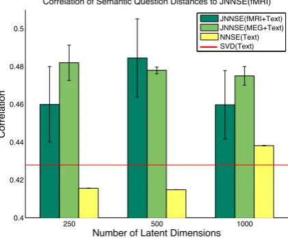
For a given value of`we solve the NNSE(Text) and JNNSE(Brain+Text) objective function as de-tailed in Equation 1 and 4 respectively. We com-pared JNNSE(Brain+Text) and NNSE(Text) mod-els by measuring the correlation of all pairwise distances in JNNSE(Brain+Text) and NNSE(Text) space to the pairwise distances in the 218-dimensional semantic space. Distances were calculated using normalized Euclidean distance (equivalent in rank-ordering to cosine distance, but more suitable for sparse vectors). Figure 1 shows the results of this correlation test. The er-ror bars for the JNNSE(Brain+Text) models rep-resent a 95% confidence interval calculated using the standard error of the mean (SEM) over the 9 person-specific JNNSE(Brain+Text) models. Be-cause there is only one NNSE(Text) model for each dimension setting, no SEM can be calculated, but it suffices to show that the NNSE(Text) corre-lation does not fall into the 95% confidence inter-val of the JNNSE(Brain+Text) models. The SVD matrix for the original corpus data has correlation 0.4279 to the behavioral data, also below the 95% confidence interval for all JNNSE models. The re-sults show that a model that incorporates brain ac-tivation data is more faithful to a behavioral mea-sure of semantics.

5.2 Word Prediction from Brain Activation

We now show that the JNNSE(Brain+Text) vec-tors are more consistent with independent sam-ples of brain activity collected from different sub-jects, even when recorded using different record-ing technologies. As previously mentioned, be-cause there is a large degree of variation between brains and because MEG and fMRI measure very different correlates of neuronal activity, this type of generalization has proven to be very challeng-ing and is an open research question in the neuro-science community.

Table 1: A Comparison of the models explored in this paper, and the data upon which they operate.

Model Name Section(s) Text Data Brain Data Withheld Data

NNSE(Text) 2, 5 X x

-NNSE(Brain) 2, 5.2.1, 5.3 x X

-JNNSE(Brain+Text) 3, 5 X X

-JNNSE(Brain+Text): Dropout task 5.2.2 X X subset of brain data

JNNSE(Brain+Text): Predict corpus 5.3 X X subset of text data

250 500 1000

0.4 0.42 0.44 0.46 0.48 0.5

Correlation of Semantic Question Distances to JNNSE(fMRI)

Number of Latent Dimensions

Correlation

JNNSE(fMRI+Text) JNNSE(MEG+Text) NNSE(Text) SVD(Text)

Figure 1: Correlation of JNNSE(Brain+Text) and NNSE(Text) models with the distances in a se-mantic space constructed from behavioral data. Error bars indicate SEM.

NNSE(Text) algorithm can be used as a VSM, which we use for the task of word prediction from fMRI or MEG recordings. A JNNSE(Brain+Text) created with a particular human subject’s data is never used in the prediction framework with that same subject. For example, if we use fMRI data from subject 1 to create a JNNSE(fMRI+Text), we will test it with the remaining 8 fMRI subjects, but all 9 MEG subjects (fMRI and MEG subjects are disjoint).

Let us call the VSM learned with JNNSE(Brain+Text) or NNSE(Text) the

se-mantic vectors. We can train a weight matrixW

that predicts the semantic vectoraof a word from that word’s brain activation vector x: a = Wx. W can be learned with a variety of methods, we will useL2 regularized regression. One can also

train regressors that predict the brain activation data from the semantic vector: x = Wa, but we have found this to give lower predictive accuracy. Note that we must re-train our weight matrix W for each subject (instead of re-using D(b) _from

Equation 4) because testing always occurs on a different subject, and the brain activation data is not inter-subject aligned.

We train ` independent L2 regularized

regres-sors to predict the `-dimensional vectors a =

{a1. . . a`}. The predictions are concatenated

to produce a predicted semantic vector: ˆa =

{ˆa1, . . . ,ˆa`}. We assess word prediction

perfor-mance by testing if the model can differentiate be-tween two unseen words, a task named2 vs. 2

pre-diction(Mitchell et al., 2008; Sudre et al., 2012).

We choose the assignment of the two held out se-mantic vectors (a(1)_,a(2)_{) to predicted semantic}

vectors (ˆa(1)_,ˆa(2)_{) that minimizes the sum of the}

two normalized Euclidean distances. 2 vs. 2 ac-curacy is the percentage of tests where the correct assignment is chosen.

The 60 nouns fall into 12 word categories. Words in the same word category (e.g. screw-driver and hammer) are closer in semantic space than words in different word categories, which makes some 2 vs. 2 tests more difficult than oth-ers. We choose 150 random pairs of words (with each word represented equally) to estimate the dif-ficulty of a typical word pair, without having to test all 60₂ word pairs. The same 150 random pairs are used for all subjects and all VSMs. Ex-pected chance performance on the 2 vs. 2 test is 50%.

250 500 1000 64

66 68 70 72 74

Number of Latent Dimensions

2 vs. 2 Accuracy

2 vs. 2 Acc. for JNNSE and NNSE, tested on fMRI data

JNNSE(fMRI+Text) JNNSE(MEG+Text) NNSE(Text) SVD(Text)

Figure 2: Average 2 vs. 2 accuracy for

NNSE(Text) and JNNSE(Brain+Text), tested on fMRI data. Models created with one subject’s fMRI data were not used to compute 2 vs. 2 ac-curacy for that same subject.

250 500 1000

66 68 70 72 74 76 78 80 82

Number of Latent Dimensions

2 vs. 2 Accuracy

2 vs. 2 Acc. for JNNSE and NNSE, tested on MEG data

JNNSE(fMRI+Text) JNNSE(MEG+Text) NNSE(Text) SVD(Text)

Figure 3: Average 2 vs. 2 accuracy for

NNSE(Text) and JNNSE(Brain+Text), tested on MEG data. Models created with one subject’s MEG data were not used to compute 2 vs. 2 ac-curacy for that same subject.

NNSE(Text) performance decreases as the number of latent dimension increases. This im-plies that without the regularizing effect of brain activation data, the extra NNSE(Text) dimensions are being used to overfit to the corpus data, or possibly to fit semantic properties not detectable with current brain imaging technologies. How-ever, when brain activation data is included, in-creasing the number of latent dimensions strictly increases performance for JNNSE(fMRI+Text). JNNSE(MEG+Text) has peak performance with 500 latent dimensions, with ∼ 1% decrease in performance at 1000 latent dimensions. In previ-ous work, the ability to decode words from brain activation data was found to improve with added latent dimensions (Murphy et al., 2012a). Our results may differ because our words are POS tagged, and we included only nouns for the final NNSE(Text) model. We found that with the orig-inalλ = 0.05 setting from Murphy et al. (Mur-phy et al., 2012a) produced vectors that were too sparse; four of the 60 test words had all-zero vec-tors (JNNSE(Brain+Text) models did have any all-zero vectors). To improve the NNSE(Text) vectors for a fair comparison, we reducedλ= 0.025, un-der which NNSE(Text) did not produce any all-zero vectors for the 60 words.

Our results show that brain activation data con-tributes additional information, which leads to an increase in performance for the task of word pre-diction from brain activation data. This suggests

that corpus-only models may not capture all rel-evant semantic information. This conflicts with previous studies which found that semantic vec-tors culled from corpus statistics contain all of the semantic information required to predict brain ac-tivation (Bullinaria and Levy, 2013).

5.2.1 Prediction from a Brain-only Model

5.2.2 Effect on Rows Without Brain Data

It is possible that some JNNSE(Brain+Text) di-mensions are being used exclusively to fit brain activation data, and not the semantics represented in both brain and corpus data. If a particular dimension j is solely used for brain data, the sparsity constraint will favor solutions that sets A_(i,j) = 0 fori > w0 _{(no brain data constraint),}

andA_(i,j) > 0 for some0 ≤ i ≤ w0 _{(brain data}

constrained). We found that there were no such dimensions in the JNNSE(Brain+Text). In fact for

the ` = 1000 JNNSE(Brain+Text), all latent

di-mensions had greater than ∼ 25% non-zero en-tries, which implies that all dimensions are being shared between the two data inputs (corpus and brain activation), and are used to reconstruct both. To test that the brain activation data is truly in-fluencing rows ofAnot constrained by brain acti-vation data, we performed adropouttest. We split the original 60 words into two 30 word groups (as evenly as possible across word categories). We trained JNNSE(fMRI+Text) with 30 words, and tested word prediction with the remaining 8 sub-jects and the other 30 words. Thus, the training and testing word sets are disjoint. Because of the reduced size of the training data, we did see a drop in performance, but JNNSE(fMRI+Text) vectors still gave word prediction performance 7% higher than NNSE(Text) vectors. Full results appear in the supplementary material.

5.3 Predicting Corpus Data

Here we ask: can an accurate latent representa-tion of a word be constructed using only brain activation data? This task simulates the scenario where there is no reliable corpus representation of a word, but brain data is available. This scenario may occur for seldom-used words that fall below the thresholds used for the compilation of corpus statistics. It could also be useful for acronym to-kens (lol, omg) found in social media contexts where the meaning of the token is actually a full sentence.

We trained a JNNSE(fMRI+Text) with brain data for all 60 words, but withhold the corpus data for 30 of the 60 words (as evenly distributed as possible amongst the 12 word categories). The brain activation data for the 30 withheld words will allow us to create latent representations in A for withheld words. Simultaneously, we will learn a mapping from the latent representation to the corpus data (D(c)_{). This task cannot be}

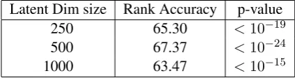
per-Table 2: Mean rank accuracy over 30 words using corpus representations predicted by a JNNSE(MEG+Text) model trained with some rows of the corpus data withheld. Significance is calculated using Fisher’s method to combine p-values for each of the subject-dependent models.

Latent Dim size Rank Accuracy p-value

250 65.30 <10−19

500 67.37 <10−24

1000 63.47 <10−15

formed with a NNSE(Text) model because one cannot learn a latent representation of a word with-out data of some kind. This further emphasizes the impact of brain imaging data, which will allow us to generalize to previously unseen words in corpus space.

We use the latent representations inAfor each of the words without corpus data and the mapping to corpus space D(c) _{to predict the withheld}

cor-pus data inX. We then rank the withheld rows of Xby their distance to the predicted row ofXand calculate the mean rank accuracy of the held out words. Results in Table 2 show that we can recre-ate the withheld corpus data using brain activation data. Peak mean rank accuracy (67.37) is attained

at` = 500 latent dimensions. This result shows

that neural semantic representations can create a latent representation that is faithful to unseen cor-pus statistics, providing further evidence that the two data sources share a strong common element. How much power is the remaining corpus data supplying in scenarios where we withhold cor-pus data? To answer this question, we trained an NNSE(Brain) model on 30 words of brain activa-tion, and then trained a regressor to predict cor-pus data from those latent brain-only representa-tions. We use the trained regressor to predict the corpus data for the remaining 30 words. Peak per-formance is attained at` = 10latent dimensions, giving mean rank accuracy of62.37, significantly worse than the model that includes both corpus and brain activation data (67.37).

5.4 Mapping Semantics onto the Brain

Because our method incorporates brain data into an interpretable semantic model, we can directly map semantic concepts onto the brain. To do this, we examined the mappings from the latent space to the brain space viaD(b)_{. We found that}

mod-!"#$%&'()

(a)D(b) _{matrix, subject P3, dimension with top words} bath-room, balcony, kitchen. MNI coordinates z=-12 (left) and z=-18 (right). Fusiform is associated with shelter words.

!"#$%&'$()*+

!(&%&'$()*+

(b)D(b) _{matrix; subject P1; dimension with top words ankle,} elbow, knee. MNI coordinates z=60 (left) and z=54 (right). Pre-and post-central areas are activated for body part words.

!"#$% &'(#)*+"#,$%

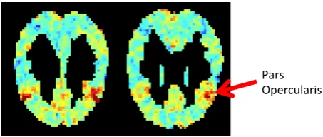
(c)D(b)_{matrix; subject P1; dimension with top scoring words} buffet, brunch, lunch. MNI coordinates z=30 (left) and z=24 (right). Pars opercularis is believed to be part of the gustatory cortex, which responds to food related words.

Figure 4: The mappings (D(b)_{) from latent}

se-mantic space (A) to brain space (Y) for fMRI and words from three semantic categories. Shown are representations of the fMRI slices such that the back of the head is at the top of the image, the front of the head is at the bottom.

els where the perceptual features had been scaled down (divided by a constant factor), which en-courages more of the data to be explained by the semantic features in A. Figure 4 shows the mappings (D(b)_{) for dimensions related to}

shel-ter, food and body parts. The red areas align with areas of the brain previously known to be activated by the corresponding concepts (Mitchell et al., 2008; Just et al., 2010). Our model has learned these mappings in an unsupervised setting by relating semantic knowledge gleaned from word usage to patterns of activation in the brain. This illustrates how the interpretability of

JNNSE can allow one to explore semantics in the human brain. The mappings for one subject are available for download (http://www.cs. cmu.edu/˜afyshe/papers/acl2014/).

6 Future Work and Conclusion

We are interested in pursuing many future projects inspired by the success of this model. We would like to extend the JNNSE algorithm to incorporate data from multiple subjects, multiple modalities and multiple experiments with non-overlapping words. Including behavioral data and image data is another possibility.

We have explored a model of semantics that in-corporates text and brain activation data. Though the number of words for which we have brain acti-vation data is comparatively small, we have shown that including even this small amount of data has a positive impact on the learned latent representa-tions, including for words without brain data. We have provided evidence that the latent representa-tions are closer to the neural representation of se-mantics, and possibly, closer to semantic ground truth. Our results reveal that there are aspects of semantics not currently represented in text-based VSMs, indicating that there may be room for im-provement in either the data or algorithms used to create VSMs. Our findings also indicate that using the brain as a semantic test can separate models that capture this additional semantic information from those that do not. Thus, the brain is an im-portant source of both training and testing data.

Acknowledgments

This work was supported in part by NIH un-der award 5R01HD075328-02, by DARPA unun-der award FA8750-13-2-0005, and by a fellowship to Alona Fyshe from the Multimodal Neuroimag-ing TrainNeuroimag-ing Program funded by NIH awards T90DA022761 and R90DA023420.

References

Andrew J Anderson, Elia Bruni, Ulisse Bordignon, Massimo Poesio, and Marco Baroni. 2013. Of words , eyes and brains : Correlating image-based distributional semantic models with neural

represen-tations of concepts. InProceedings of the

Confer-ence on Empirical Methods on Natural Language Processing.

David M Blei and Jon D. McAuliffe. 2007. Supervised

topic models. In Advances in Neural Information

Elia Bruni, Giang Binh Tran, and Marco Baroni. 2011. Distributional semantics from text and images. In

Proceedings of the EMNLP 2011 Geometrical Mod-els for Natural Language Semantics (GEMS). John A Bullinaria and Joseph P Levy. 2013. Limiting

factors for mapping corpus-based semantic

repre-sentations to brain activity. PloS one, 8(3):e57191,

January.

Jamie Callan and Mark Hoy. 2009. The ClueWeb09 Dataset.

Jonathan Chang, Jordan Boyd-Graber, Sean Gerrish, Chong Wang, and David M Blei. 2009. Reading Tea Leaves : How Humans Interpret Topic Models. InAdvances in Neural Information Processing

Sys-tems, pages 1–9.

Kenneth Ward Church and Patrick Hanks. 1990. Word association norms, mutual information, and

lexicog-raphy.Computational linguistics, 16(1):22–29.

Bryan R Conroy, Benjamin D Singer, J Swaroop Gun-tupalli, Peter J Ramadge, and James V Haxby. 2013. Inter-subject alignment of human cortical anatomy

using functional connectivity. NeuroImage, 81:400–

11, November.

Andrew D Engell, Scott Huettel, and Gregory Mc-Carthy. 2012. The fMRI BOLD signal tracks elec-trophysiological spectral perturbations, not

event-related potentials. NeuroImage, 59(3):2600–6,

February.

Alona Fyshe, Partha Talukdar, Brian Murphy, and Tom Mitchell. 2013. Documents and Dependencies : an Exploration of Vector Space Models for Semantic

Composition. InComputational Natural Language

Learning, Sofia, Bulgaria.

Arthur M Glenberg and David a Robertson. 2000. Symbol Grounding and Meaning: A Compari-son of High-Dimensional and Embodied Theories

of Meaning. Journal of Memory and Language,

43(3):379–401, October.

Sunil Kumar Gupta, Dinh Phung, Brett Adams, and Svetha Venkatesh. 2013. Regularized nonnegative

shared subspace learning. Data Mining and

Knowl-edge Discovery, 26(1):57–97.

Emma L Hall, Siˆan E Robson, Peter G Morris, and Matthew J Brookes. 2013. The relationship

be-tween MEG and fMRI.NeuroImage, November.

Harold Hotelling. 1936. Relations between two sets of

variates. Biometrika, 28(3/4):321–377.

Yangqing Jia and Trevor Darrell. 2010. Factorized

La-tent Spaces with Structured Sparsity. InAdvances in

Neural Information Processing Systems, volume 23. Marcel Adam Just, Vladimir L Cherkassky, Sandesh Aryal, and Tom M Mitchell. 2010. A neuroseman-tic theory of concrete noun representation based on

the underlying brain codes. PloS one, 5(1):e8622,

January.

Nikolaus Kriegeskorte, Marieke Mur, and Peter Ban-dettini. 2008a. Representational similarity analysis - connecting the branches of systems neuroscience.

Frontiers in systems neuroscience, 2(November):4, January.

Nikolaus Kriegeskorte, Marieke Mur, Douglas A Ruff, Roozbeh Kiani, Jerzy Bodurka, Hossein Esteky, Keiji Tanaka, and Peter A Bandettin. 2008b. Match-ing Categorical Object Representations in Inferior

Temporal Cortex of Man and Monkey. Neuron,

60(6):1126–1141.

TK Landauer and ST Dumais. 1997. A solution to Plato’s problem: The latent semantic analysis the-ory of acquisition, induction, and representation of

knowledge. Psychological review, 1(2):211–240.

Julien Mairal, Francis Bach, J Ponce, and Guillermo Sapiro. 2010. Online learning for matrix

factor-ization and sparse coding. The Journal of Machine

Learning Research, 11:19–60.

Ken McRae, George S Cree, Mark S Seidenberg, and Chris McNorgan. 2005. Semantic feature produc-tion norms for a large set of living and nonliving

things. Behavior research methods, 37(4):547–59,

November.

Tom M Mitchell, Svetlana V Shinkareva, Andrew Carl-son, Kai-Min Chang, Vicente L Malave, Robert A

Mason, and Marcel Adam Just. 2008.

Pre-dicting human brain activity associated with the

meanings of nouns. Science (New York, N.Y.),

320(5880):1191–5, May.

Brian Murphy, Partha Talukdar, and Tom Mitchell. 2012a. Learning Effective and Interpretable Se-mantic Models using Non-Negative Sparse

Embed-ding. In Proceedings of Conference on

Computa-tional Linguistics (COLING).

Brian Murphy, Partha Talukdar, and Tom Mitchell. 2012b. Selecting Corpus-Semantic Models for

Neu-rolinguistic Decoding. In First Joint Conference

on Lexical and Computational Semantics (*SEM), pages 114–123, Montreal, Quebec, Canada.

Andrew Y. Ng and Michael I. Jordan. 2002. On dis-criminative vs. generative classifiers: A

compari-son of logistic regression and naive bayes. In

Ad-vances in neural information processing systems, volume 14.

Mark Palatucci, Geoffrey Hinton, Dean Pomerleau, and Tom M Mitchell. 2009. Zero-Shot Learning

with Semantic Output Codes. Advances in Neural

Information Processing Systems, 22:1410–1418.

Rajeev D S Raizada and Andrew C Connolly. 2012. What Makes Different People’s Representations Alike : Neural Similarity Space Solves the Problem

of Across-subject fMRI Decoding. Journal of

Indrayana Rustandi, Marcel Adam Just, and Tom M

Mitchell. 2009. Integrating Multiple-Study

Multiple-Subject fMRI Datasets Using Canonical

Correlation Analysis. InMICCAI 2009 Workshop:

Statistical modeling and detection issues in intra-and inter-subject functional MRI data analysis.

Magnus Sahlgren. 2006. The Word-Space Model

Us-ing distributional analysis to represent syntagmatic and paradigmatic relations between words. Doctor of philosophy, Stockholm University.

Carina Silberer and Mirella Lapata. 2012. Grounded

models of semantic representation. InProceedings

of the 2012 Joint Conference on Empirical Methods in Natural Language Processing and Computational Natural Language Learning, pages 1423–1433. Carina Silberer, Vittorio Ferrari, and Mirella Lapata.

2013. Models of Semantic Representation with

Vi-sual Attributes. In Association for Computational

Linguistics 2013, Sofia, Bulgaria.

Gustavo Sudre, Dean Pomerleau, Mark Palatucci, Leila Wehbe, Alona Fyshe, Riitta Salmelin, and Tom Mitchell. 2012. Tracking Neural Coding of Per-ceptual and Semantic Features of Concrete Nouns.

NeuroImage, 62(1):463–451, May.

Peter D Turney and Patrick Pantel. 2010. From Fre-quency to Meaning : Vector Space Models of

Se-mantics. Journal of Artificial Intelligence Research,

37:141–188.

Martha White, Yaoliang Yu, Xinhua Zhang, and Dale Schuurmans. 2012. Convex multi-view subspace

learning. In Advances in Neural Information