Multiple days ahead value at risk and expected shortfall forecasting for stock indices, commodities and exchange rates: inter day versus intra day data

(1)

Munich Personal RePEc Archive

Multiple-days-ahead value-at-risk and

expected shortfall forecasting for stock

indices, commodities and exchange rates:

inter-day versus intra-day data

Degiannakis, Stavros and Potamia, Artemis

Department of Economic and Regional Development, Panteion

University, Greece

1 January 2017

Online at

https://mpra.ub.uni-muenchen.de/96278/

(2)

Multiple-days-ahead value-at-risk and expected shortfall forecasting for stock indices, commodities and exchange rates: Inter-day versus Intra-day data

Abstract

In order to provide reliable Value-at-Risk (VaR) and Expected Shortfall (ES) forecasts, this paper attempts to investigate whether an inter-day or an intra-day model provides accurate predictions. We investigate the performance of inter-day and intra-day volatility models by estimating the AR(1)-GARCH(1,1)-skT and the AR(1)-HAR-RV-skT frameworks, respectively. This paper is based on the recommendations of the Basel Committee on Banking Supervision. Regarding the forecasting performances, the exploitation of intra-day information does not appear to improve the accuracy of the and forecasts for the 10-steps-ahead and 20-steps-ahead for the 95%, 97.5% and 99% significance levels. On the contrary, the GARCH specification, based on the inter-day information set, is the superior model for forecasting the multiple-days-ahead and measurements. The intra-day volatility model is not as appropriate as it was expected to be for each of the different asset classes; stock indices, commodities and exchange rates.

The multi-period and forecasts are estimated for a range of datasets (stock indices, commodities, foreign exchange rates) in order to provide risk managers and financial institutions with information relating the performance of the inter-day and intra-day volatility models across various markets. The inter-day specification predicts and measures adequately at a 95% confidence level. Regarding the 97.5% confidence level that has been recently proposed in the revised 2013 version of Basel III, the GARCH-skT specification provides accurate forecasts of the risk measures for stock indices and exchange rates, but not for commodities (i.e. Silver and Gold). In the case of the 99% confidence level, we do not achieve sufficiently accurate and forecasts for all the assets.

Keywords: Basel II, Basel III, Value-at-Risk, Expected Shortfall, volatility forecasting, intra-day data, multi-period-ahead, forecasting accuracy, risk modelling.

(3)

1. Introduction and review of the literature

Risk management has now become a standard prerequisite for all financial institutions. Value-at-Risk (VaR) is the main risk management tool used to compute the risk of financial assets accurately. More specifically, VaR refers to the worst outcome of a portfolio that is likely to occur at a given confidence level over a specified period, and it focuses on market risk; see Angelidis and Degiannakis (2007). There are three methods of calculating VaR; the first category refers to the major representatives of parametric family, which are the Autoregressive Conditional Heteroskedasticity (ARCH) models. The second category, non-parametric

modeling, relies on actual prices without assuming any specific distribution, and the main

representative of this category is the historical simulation. The last category is the

semi-parametric family that combines the two aforementioned frameworks. With regard to the

appropriate methods of model evaluation, there are two main ones: the evaluation of the statistical properties of VaR forecasts, and the construction of a loss function that measures the distance between the predicted VaR and the actual portfolio outcome.

It is also significant that the VaR measurement has been adopted by bank regulators. Specifically, according to the Basel Committee on Banking Supervision (1995a,1995b, 2009), the VaR methodology can be used by financial institutions to calculate capital charges in accordance with their financial risk. These institutions could determine their daily capital charge by following the three prerequisites: a) The 99% confidence level must be usedto make sure that institutions hold enough capital to ensure a safe and efficient market able to withstand any foreseeable problems. b) The minimum holding period must be set to 10 trading days, so that investors are able to liquidate their positions due to price changes. c) Banks could calculate VaR

by implementing internal models.

In general, the Basel’s II VaR quantitative requirements include: a) daily-basis estimation, b) confidence level set of 99%, c) minimum sample extension of a one year with quarterly or more frequent updates, d) no specific models prescribed, for instance, banks are free to adopt their own schemes, e) regular backtesting program for validation purposes.

(4)

One of the most important issues in finance is the choice of one benchmark volatility model to forecast the risk that an investor faces. Since Engle’s (1982) seminal paper, many other researchers have tried to find the most appropriate risk model that predicts future variability of asset returns by employing various specifications based on ARCH models, using data of different financial markets. Hence, their results are confusing and conflicting, because there is no model that is deemed adequate for all financial datasets, distributions, sample frequencies and applications. In addition, most of the empirical works are based on daily returns. Some of the most quintessential studies in the literature are presented in the following paragraphs.

Giot and Laurent (2003a), who proposed the asymmetric power of ARCH with skewed Student-t distributed innovations or the APARCH-skT model, estimated the daily VaR for stock portfolios. The findings conducted from this research performed better results for the skewed Student-t distribution than the pure, symmetric one. Although Giot and Laurent (2003b) kept the same distributional assumption, they chose another dataset, that of six commodities. They also claimed that more complex models (e.g. APARCH) performed better overall. Brooks and Persand (2003) concluded that the models which do not allow for asymmetries underestimate the true VaR.

Degiannakis (2004) suggested the fractionally integrated APARCH (FIAPARCH) model and stated that the FIAPARCH with skewed Student-t distributed innovations produces the most accurate one-day-ahead VaR predictions among three European stock indices (CAC40, DAX30 and FTSE100). Degiannakis et al. (2013) investigated a set of 20 stock indices worldwide and provided evidence that the fractional integration in the conditional variance model does not improve the accuracy of the VaR forecasts relative to the short memory GARCH specification. Additionally, other researchers, such as Angelidis et al. (2004) and McMillan and Kambouroudis (2009) proposed different volatility structures to estimate the daily VaR, but yet again without reaching a consensus and a common conclusion. They argued that the choice of the best performing model depends on the equity index. Hansen and Lunde (2005a) investigated DM-$ exchange rates and IBM stock returns and concluded that there is no evidence that the GARCH(1,1) model is outperformed by other models when the models are evaluated using the exchange rate data. This cannot be explained by the SPA test, as the ARCH(1) model is clearly rejected and found to be inferior to other models. In the analysis of IBM stock returns they found conclusive evidence that the GARCH(1,1) is inferior, and suggested that out-of-sample performance requires a specification that can accommodate a leverage effect.

(5)

Laurent (2004) compared the APARCH-skT model with an ARFIMAX specification, in their attempt to capture VaR for stock indices and exchange rates as well. They conclude that the use of an intra-day dataset did not improve the performance of the inter-day VaR model, a fact analyzed in depth in this paper, looking not only at stocks as is the norm, but also at an extended dataset consisting of stock indices, commodities and exchange rates. Another important study that strengthens the results of the present study is that of Giot (2005), who estimated VaR at intra-day time horizons of 15 and 30 minutes. He proposed that the GARCH model with skewed Student-t distributed innovations had the best overall performance and that there were no significant differences between daily and intra-day VaR models once the intra-day seasonality in volatility was taken into account.

Although there is a plethora of forecasting models, the financial institutions have to abide by the recommendations of the Basel Committee on Banking Supervision. We have chosen the AR(1)-GARCH(1,1) model, a short memory model, which we compare to the Heterogeneous Autoregressive Realized Volatility, AR(1)-HAR-RV, model based on intra-day high frequency data. The distribution of the two models is the skewed Student-t (skT). Regarding the frequency of these forecasts, we have used 10-days-ahead and 20-days-ahead

and forecasts1 for both models, at the 95%, 97.5% and 99% confidence level. Therefore, we will be able to study the VaR and ES forecasts at the confidence level of 97.5%, as was recently proposed in Basel III, revised in 2013, and compare them with the risk measures at the confidence level of 99%, as it has been proposed in Basel II. In support of our choice of GARCH(1,1), many researchers including Bollerslev (1986), Engle (2004), Giot and Laurent (2004) have pointed out that it has been shown to produce accurate VaR forecasts, among all the inter-day models, across a variety of markets and under different distributional assumptions. Some of the studies also concluded that the use of a skewed instead of a symmetrical distribution at a GARCH specification for the standardized residuals produces superior VaR forecasts, i.e. Giot and Laurent (2003a), Angelidis et al. (2004) and Degiannakis et al. (2014).

The HAR-RV model offers many advantages. First of all, the model retains a structure that enables the realized volatility estimates to be aggregated on different scales in order to find the realized volatility measures of the integrated volatility over different periods: daily, weekly and monthly. This is a strong advantage and the reason is simple. Typically, a financial market is comprised of participants with a large spectrum of dealing frequency. On one end of the dealing spectrum there are dealers, market makers and intraday speculators who are interested in forecasting intraday frequency data, on a daily or weekly basis. On the other end, there are central banks, commercial organization and pension fund investors, who, in their attempt to employ currency hedging, need to forecast high frequency data in a long-run period of at least a

1

(6)

month. Each such participant has a different reaction to the news related to his/her investment horizon. The basic idea is that agents with different time horizons perceive, react and cause different types of volatility components, as Corsi (2002) has mentioned. Simplifying a little, the model of HAR-RV can easily identify three primary volatility components: the short-term with daily or higher trading frequency, the medium-term typically made up of portfolio managers who rebalance their positions weekly, and the long-term with a characteristic time of one month or more. Moreover, HAR can be estimated easily, as it is a multiple regression model. Surprisingly, although it does not formally belong to the class of long-memory models, the HAR-RV model is able to reproduce the same memory persistence observed in volatility (see Corsi, 2009).

The purpose of this research is to investigate the predictive ability of these models in multi-period forecasting horizons (being in line with the Basel Committee suggestion for a minimum period of 10 trading days) across a variety of markets; stocks, commodities and exchange rates. There is not an extensive literature on VaR and ES forecasting based on intra-day data2. Moreover, the majority of the studies dealing with intra-day volatility measures focus either on one-day-ahead VaR forecasts3, or on the analysis of a limited dataset4.

To summarize, for 10-days-ahead and 20-days-ahead forecasts of risk measures, the inter-day GARCH model is superior. On the other hand, the intra-inter-day model suffers from excessive

VaR violations, implying an underestimation of market risk. Undoubtedly, the inter-day GARCH specification is a safe model to adequately predict market risk measures at a 95% confidence level. The multi period-ahead VaR and ES forecasts are more accurate at the confidence level of 97.5% (as suggested in the revised version of Basel III in 2013) than at the confidence level of 99% (proposed in Basel II). Finally, a new innovative inference has emerged; the choice of the GARCH-skT has been shown to produce reasonable multiple-days-ahead and forecasts under the skewed Student-t distribution, and most importantly, across a variety of asset classes.

The structure of the paper is as follows: Section 2 describes the VaR and ES forecasting frameworks through an ARCH process (inter-day modeling). Section 3 presents the construction of the and multiple-days-ahead forecasts under a HAR specification (intra-day modeling). Section 4 describes the evaluation methods of and forecasts. Section 5 gives a description of the daily log-returns and the intra-day based realized volatility measures. Section 6 investigates the empirical results of the analysis. Section 7 concludes the paper, providing the final outcomes of this research.

2_{The most representative studies of intra-day based}_VaR_{modelling are Giot and Laurent (2004),}

Koopman et al. (2005), Beltratti and Morana (2005), Angelidis and Degiannakis (2008), Martens et al.

(2009), Louzis et al., (2013).

3

I.e. Krzemienowski and Szymczyk (2016), Nadarajah et al. (2016), Su (2015), Watanabe (2012).

4

(7)

2. Multiple-days-ahead and forecasts under an ARCH specification (inter-day modelling)

As part of the literature on risk management and forecasting, ARCH models are used to characterize and model the financial time series. In 2003, Robert F. Engle was awarded the Nobel Prize for his pioneering work on ARCH volatility modeling. Let

refer to the continuously compounded return series, where is the closing price of the trading day t. The return series follows the stochastic process:

(1)

where denotes the conditional mean, given the information available, ,

is the ARCH process with unconditional variance and conditional variance

, is the density function of , is a positive measurable functional form (i.e. the ARCH volatility dynamic structure) and θ is the vector of the unknown parameters.

Because the distribution of asset returns is not symmetric, parametric VaR models faced difficulties in correctly modeling the tails of the distribution of returns. As a result, Angelidis and Degiannakis (2005), Giot and Laurent (2003a) and Lambert and Laurent (2001), among others, proposed the use of the skewed Student-t Distribution, so as to take into account the fat and platykurtic tails of the log-returns.

The τ-days-ahead for a long trading position at level of confidence is expressed as:

(2)

Although the VaR gives important information about potential loss, it does not indicate information about expected loss. Thus, Artzner et.al. (1997), Artzner et al. (1999) and Delbaen (2002) introduced the ES risk measure.

ES is the expected value of loss, given that a VaR violation occurs, or in other words the conditional expectation of loss that takes into account losses beyond the VaR level.

The τ-days-ahead for a long trading position is expressed as:

. (3)

Moreover, ES is a coherent risk measure, which satisfies the properties of sub-additivity, homogeneity, monotonicity and risk-free condition.

(8)

conditional mean is specified as a 1st order autoregressive process in order to allow for the non-synchronous trading effect5 (see Degiannakis et al., 2013, Lo and MacKinlay, 1990). Furthermore, we utilize the density function of skewed Student-t in order to take into account the fat tails and the asymmetry of the returns. The skewed Student-t distribution was extended to the GARCH framework by Lambert and Laurent (2000, 2001), who based their work on that of Hansen (1994). Consequently, a Monte Carlo algorithm for computing

under the AR(1)-GARCH(1,1)-skT model is presented, based on Xekalaki and Degiannakis (2010) and Christoffersen (2003):

(4)

where g and ν are the asymmetry and tail parameters of the distribution,

_and _{. The}

denotes the density function of the Student-t distribution6.

The Monte Carlo simulation algorithm for computing the τ-days-ahead

forecasts based on the AR(1)-GARCH(1,1)-skT model is obtained as following:

One – day – ahead

Step 1: Compute the one-day-ahead conditional standard deviation:

.

(5)

Step 2: Generate random numbers,

from the skewed Student-t distribution, where

MC=5000 denotes the number of draws.

Step 3: Simulate the one-trading day ahead log-returns in accordance to the AR(1) progress:

, for . (6) τ-day-ahead7

5

The non-synchronous trading effect, first analyzed by Fisher (1966), expresses the autocorrelation presented in financial time series due to the fact that the values have been recorded at time intervals of one length but were recorded at time intervals of another, not necessarily regular, length.

6

Thus, for example,

. For more details, the reader

(9)

Step τ.1: Generate random numbers, from the skewed Student-t distribution.

Step τ.2: Create the forecast standard deviation of trading day t+τ:

.

(7)

Step τ.3: Simulate the unpredictable component: . Step τ.4: Create the hypothetical returns of time t+τ, as:

, for . (8)

Step τ: Calculate the τ-days-ahead and as:

, and (9)

(10)

3. Multiple-days-ahead and forecasts under a HAR specification (intra-day modeling)

The availability of ultra-high frequency data rekindled the interest of many researchers in risk forecasting. This is illustrated by the fact that the squared daily returns are an unbiased but noisy estimator of volatility. Many researchers employ ultra-high frequency data in order to extract more information, which enables them to forecast daily VaR accurately. Andersen and Bollerslev (1998) showed that daily realized volatility may be constructed simply by summing up intra-day squared log-returns. Additionally, the contribution of Corsi (2009), who introduced the Heterogeneous Autoregressive for Realized Volatility (HAR-RV) model, is depicted as one of the quintessential processes. The HAR-RV model is an autoregressive structure of the realized volatilities over different time intervals. The HAR-RV model for the logarithmic

transformation of the annualized realized volatility , is defined as:

(11)

where . The accounts for the volatility perception from inter-day and intra-day

traders, whereas the accounts for medium term trading strategies. Moreover, the

encompasses the perception of volatility for investment strategies with monthly or even longer time horizons. The heterogeneity is the reason of the volatility variations through different time intervals.

7

(10)

The AR(1)-HAR-RV-skT model is defined as an AR(1) process for the daily

log-returns, + . The unpredictable component , is designed to follow the skewed Student-t distribution conditional on the most recently available information set, or

. Moreover, the unpredictable component is

decomposed as . Hence, the AR(1)-HAR-RV-skT model is defined as:

(12)

(13)

(14)

The Monte Carlo simulation algorithm for computing the forecasts based on the AR(1)-HAR-RV-skT model is illustrated:

One – day – ahead

Step 1: Compute the one-day-ahead realized volatility according to equation (13). Note that denotes the average of i) actual values for points in time prior to t and ii) predicted values for points in time subsequent time t. The same case holds for .

Step 2: Generate MC=5000 random numbers, , from the skewed Student-t distribution.

Step 3: The value of the unpredictable component is .

Step 4: Simulate the one-trading day ahead log-returns in accordance to the AR(1) progress:

, for . (15) τ– days – ahead8

Step τ.1: Compute the τ-day-ahead realized volatility as:

(16 )

Step τ.2: Generate

from the skewed Student-t distribution.

Step τ.3: Simulate the -trading days ahead log-returns:

, for . (17)

Step τ: Calculate the τ-days-ahead and as:

8

(11)

(18)

.

(19)

4. Evaluate multiple-days-ahead and Forecasts

The VaR measure must neither overestimate nor underestimate the expected loss, as in both cases the financial institution allocates the wrong amount of capital. The simplest method to measure the accuracy of the risk models is to record the total number of violations. However, there are statistical techniques for evaluating VaR models. The quintessential ones are the methods of Kupiec (1995) and Christoffersen (1998), called backtesting procedures.

4.1.First Stage Evaluation

The test most widely used was developed by Kupiec (1995). It examines the hypothesis of whether the average number of violations is statistically equal to the excepted one. The appropriate likelihood ratio statistic is:

,

(20)

where is the number of days over a period that a violation occurred and as a result the portfolio loss was larger than the VaR estimate9, and ρ is the expected ratio of violations. The risk model will be rejected if it generates too many or too few violations:

(21)

According to Kupiec (1995), the number of violations follows a binominal distribution

and the hypotheses tested are:

,

. (22)

Christoffersen (1998) examined concurrently if the VaR failure process is independently distributed or not. The hypotheses presented on the second backtesting criterion are defined as:

,

.

(23)

The is the corresponding probability and i, j=1 denotes that a violation has

occurred, whereas i, j=0 indicates the opposite. The likelihood ratio statistics for the independence is described in the following:

. (24) The main advantage of using the above two backtesting tests is the fact that the managers could easily reject a VaR model that generates too many or too few clustered

9

(12)

violations. However, their drawback is that these two backtesting procedures cannot classify the models based only on the p-values of these tests.

4.2.Second Stage Evaluation

The limitation of backtesting tests leads to the excessive need of the second stage of evaluation forecasting. Lopez (1999) proposed a forecast evaluation framework which is focused on a loss function measuring the accuracy of VaR forecasts on the basis of the distance between the observed returns and the forecasted VaR values, given that a violation occurred. Through the Lopez (1999) approach, a VaR model is penalized when an exception takes place. Nevertheless, as Angelidis and Degiannakis (2007) noted, the returns should better be compared with ES

instead of VaR, since VaR does not imply indications concerning the size of the expected loss. So we employ a loss function that measures the squared distance between actual daily returns and the forecasts as:

(25)

The preferable model is the one that minimizes the average loss, , called the Mean Predictive Squared Error (MPSE).

Predictive accuracy is further explored with the Diebold and Mariano (1995) test10. We investigate whether the loss functions of the two models are statistically different. Let us define _and _{as the loss functions from the AR(1)-GARCH(1,1)-skT and}

AR(1)-HAR-RV-skT models, respectively. The null hypothesis that these two models are of equivalent predictive ability is tested against the alternative hypothesis that the AR(1)-GARCH(1,1)-skT model is of superior predictive ability:

.

(26)

The Diebold and Mariano statistic is computed as the test statistic of the constant coefficient

from regressing on a constant with heteroskedastic and auto correlated

consistent standard errors, or

.

5. Inter-Day and Intra-Day Data

In this paper, we use three types of financial asset classes; stock indices, commodities and foreign exchange rates. The 3 stock indices are the Standard and Poor's 500 from the US stock market (S&P500) with 3901 observations, the Europe Stock 50 (EurostoXX50) with 3949

10

(13)

observations, and the Financial Times Stock Exchange 100 from London stock market (FTSE100) with 3912 observations. The 3 commodities are Copper (HG) with 3897 observations, Silver (SV) with 3897 observations and Gold (GC), also with 3897 observations. The 3 foreign exchange rates are the Euro Exchange Rate based on the US Dollar (EUR/USD) with 3898 observations, the British Pound Exchange Rate based on the US Dollar (GBP/USD) with 3899 observations and finally, the Canadian Dollar Exchange Rate based on the US Dollar (CAD/USD) with 3899 observations11.

The data from the nine asset prices cover a range of fifteen years, spanning the period from 3 January, 2000 to 5 August, 2015 and were conditioned to remove any non-trading days. To avoid outliers that would result from half trading days, we removed days that stock markets were not active for more than six and a half hours between 9:30 a.m. and 4:00 p.m. Furthermore, inactive trading days were excluded when stock markets were closed for the whole day, such as weekends and public or local holidays; for instance, the day after Thanksgiving and days around Christmas.

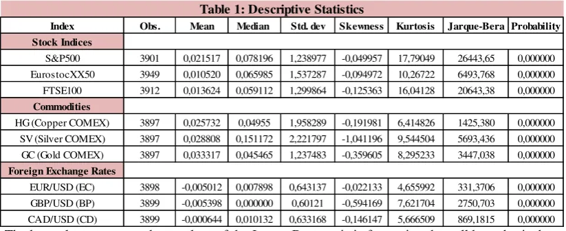
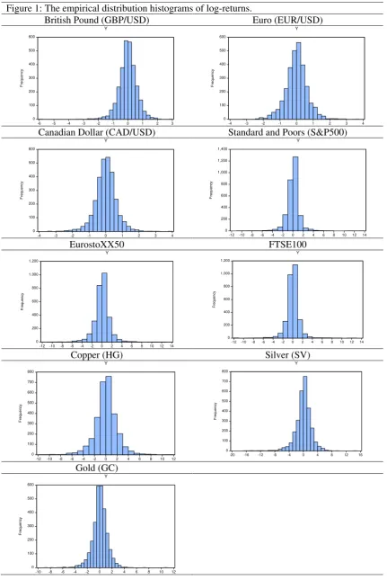
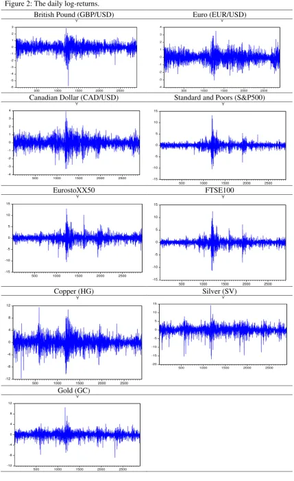
Descriptive statistics for the daily log-returns for the selected stock indices, commodities and exchange rates are presented in Table 1. All of the returns distributions are platykurtic, due to the fact that the kurtosis is a large positive value for all the nine assets. Figure 1 plots the distribution histograms of log-returns. All the asset classes are negatively skewed. The Jarque-Bera results indicate that none of the log-returns series follow a Gaussian distribution. It is clear that in almost all the graphs depicted in Figure 2 the same periods of intense volatility clustering are found. The major cluster of volatility encompasses the observations around the year of 2008 in which Lehman Brothers collapsed.

{INSERT TABLE 1} {INSERT FIGURES 1-2}

Let us define as the intra-day asset price on trading day t which has been partitioned in m

equidistance points within the trading day. The realized volatility is computed according to Hansen and Lunde (2005b) in order to scale the intra-day realized volatility with the volatility during the time that the market is closed:

. (27)

11

(14)

The term is the intra-day realized volatility, whereas

the term takes into consideration the overnight volatility. The

intra-day sampling frequency is selected based on the criterion of minimizing the intra-intra-day auto-covariance12 that approximates the measurement errors due to microstructure frictions. The

parameters and are estimated such as , as

, where is the actual but

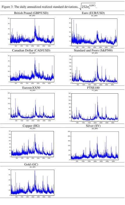
unobservable volatility; the integrated volatility13. Figure 3 plots the annualized realized standard

deviations, , for the stock indices, commodities and exchange rates, whereas the

descriptive statistics of are presented in the Table 2. The kurtosis is highly positive

for all the asset classes referring to leptokurtic distributions. Moreover, all the are

positively skewed. The descriptive statistics of the stock indices are qualitatively similar to those presented in the literature, i.e. Degiannakis and Floros (2016) have illustrated the descriptive information for 17 European and USA stock indices. Compared to stock indices, commodities are characterized by higher values of volatility, whereas exchange rates by much lower values of volatility. For example, the average daily annualized volatility of silver is 27.8% with a standard

deviation of 15.9%, which is higher than the 22.7% average of EurostoXX50 with

a standard deviation of 12.8%. On the other hand, the EUR/USD exchange rate has an average daily annualized volatility of 9.6% with a standard deviation of 4.1%.

{INSERT FIGURE 3} {INSERT TABLE 2} 6. Empirical Analysis

Τhe predictive accuracy of the AR(1)-GARCH(1,1)-skT and the AR(1)-HAR-RV-skT models is investigated, concerning the 95%, 97.5% and the 99% confidence levels. Based on the total number of T observations (trading days), the rolling window approach with a fixed window length of trading days is utilized. Hence, the models are re-estimated every trading day

t

, for days. The results for the 10-trading-days-ahead forecasts at the 95%

12

The expected value of intra-day auto covariance equals to zero; see i.e. Andersen et al. (2006). The auto-covariance is computed as , for denoting the intra-day log-returns.

13

(15)

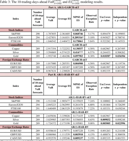
confidence level are presented in Table 3, across the 3 asset classes. Table 3 presents the average

values of and , the mean predicted squared error for , the observed

exception rate and the p-values of Kupiec and Christoffersen backtesting tests. Figure 4

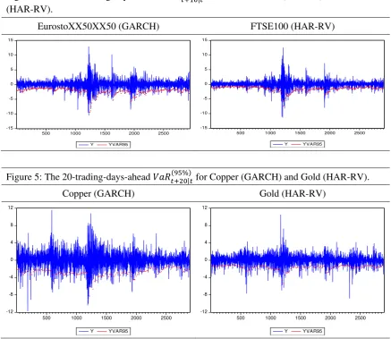
illustrates, indicatively, the log-returns and the for EurostoXX50 and FTSE100. The

relative graphs for the other assets are available from the authors on request.

For the 10-trading-days-ahead forecasting horizon, the HAR-RV-skT model does not outperform the GARCH-skT specification. The GARCH-skT model framework is slightly preferable since the observed exception rates are much closer to the expected ones. The p-values of the Kupiec test are highly acceptable in all the cases except for Gold (for both models) and Silver (for the HAR-RV-skT model). Additionally, the independence test does not reject the hypothesis that the violations are independently distributed for both model frameworks at any reasonable level of significance for all the assets except for the Gold.

Moreover, the MPSE loss function (for the predicted ) of the GARCH-skT

model is lower than that of the HAR-RV-skT model in 7 out of 9 cases. However, the statistical comparison of the predictive accuracy according to the Diebold Mariano test indicates that only

in the case of EurostoXX50 and Silver the forecasts of the GARCH-skT model are

statistically more accurate than those of the HAR-RV-skT model14. Overall, less accurate risk forecasts are estimated for Gold.

{INSERT TABLE 3} {INSERT FIGURE 4}

For the longer time horizon of 20-days-ahead, at the 95% confidence level, the results are presented in Table 4. The forecasting performance of the GARCH-skT model has not deteriorated compared to the case of 10-days-ahead predictions. On the contrary, the HAR-RV-skT model seems to provide less accurate forecasts in this time horizon, as there are more rejections of the backtesting test of Kupiec. The Kupiec statistic for the GARCH-skT model suggests that the observed exception rate is statistically equal to the expected failure rate for all the assets. However, the Kupiec test for the HAR-RV-skT model rejects the null hypothesis at a 5% level of significance in four cases; specifically, for the EurostoXX50, FTSE100, Silver and Gold. Additionally, the independence test does not reject the hypothesis that the violations are independently distributed for both model frameworks at any reasonable level of significance for all the assets. The only exception is that of the EurostoXX50, for the risk forecasts provided by the intra-day realized volatility model.

14

(16)

Turning to the estimates for the quadratic loss function that measures the squared

distance between actual returns and expected loss in the event of a violation (MPSE

loss function for forecast), the GARCH-skT model produces lower values in 6 out of 9

cases. The Diebold Mariano test provides evidence that only in the case of Silver, the

forecasts of the GARCH-skT model are statistically more accurate compared to those of the HAR-RV-skT model. Hence, the GARCH-skT specification seems to be preferable to that of the

HAR-RV-skT, as the former satisfies most of the prerequisites concerning the and

forecasting. Figure 5 illustrates, indicatively, the log-returns and the for

Copper and Gold15.

{INSERT TABLE 4} {INSERT FIGURE 5}

The results for the and measures are similar to the 95% results and

they are presented in Table 5. Overall, the daily conditional volatility model outperforms the

intra-day realized volatility model. The GARCH-skT model provides accurate

forecasts (as the p-values of the unconditional coverage test are higher than the 0.05 value) for all the indices except for the Silver and the Gold commodities. On the other hand, the

HAR-RV-skT model produces more violations than expected, not only for Silver and Gold, but

also for the FTSE100 index. Turning to the estimates of the MPSE loss function for the

, the GARCH-skT model has a lower MPSE loss function compared to that of the HAR-RV-skT model in 7 out of 9 cases. Concerning the FTSE100, Silver and Gold, the

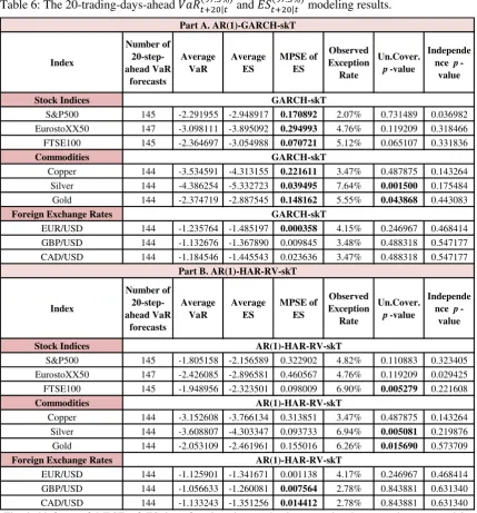
forecasts from the GARCH-skT model are statistically more accurate compared to those from the HAR-RV-skT model. Table 6 illustrates the information regarding the

and forecasts. Both models provide accurate forecasts for all the indices except for Silver and Gold, and the GARCH-skT model has a lower MPSE loss

function for the compared to that of the HAR-RV-skT model in 7 out of 9 cases

(although for all the assets, the forecasts from both models are statistically equal).

{INSERT TABLES 5-6}

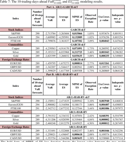
The results for the and measures are presented in Table 7. Overall,

the daily conditional volatility model outperforms the intra-day realized volatility model. But,

the GARCH-skT model provides accurate forecasts (as the p-values of the

unconditional coverage test are higher than the 0.05 value) in only 5 cases. On the other hand,

15

(17)

the HAR-RV-skT model produces more violations than expected in 7 out of 9 cases.

Turning to the estimates of the MPSE loss function for the , the GARCH-skT model has

a lower MPSE loss function compared to that of the HAR-RV-skT model in 7 out of 9 cases.

Finally, according to Table 8, qualitatively similar findings are provided for the and

forecasts as in the case of the 10-days-ahead predictions. {INSERT TABLES 7-8}

Even nowadays, the majority of the studies, i.e. Krzemienowski and Szymczyk (2016), Nadarajah et al. (2016), Su (2015), Watanabe (2012) investigate the one-day-ahead forecasting performance, but as it was mentioned before, the minimum holding period must be set to 10 trading days. To conclude, after checking the 10-steps-ahead and 20-steps-ahead forecasts of risk measures from GARCH-skT and HAR-RV-skT models, we can infer that the results for the risk models are not very clear across different asset classes. Hence, it is difficult for risk modelers to propose a clear-cut conclusion, concerning which model is the most accurate and reliable to adequately forecast the losses of a specific portfolio. After a careful examination, we observe that for the 95% confidence level, the daily conditional volatility model provides adequate and forecasts for medium-term and long-term periods, such as 10-days and 20-days-ahead16. The only exception is the case of Gold. Turning to the 97.5% confidence level, the GARCH-skT model provides adequate and forecasts for 7 of the cases but not for two of the commodities; Silver and Gold. The picture is more complicated in the case of the 99% confidence level, which is much more difficult to forecast accurately. At the 99% confidence level, although the GARCH-skT model outperforms the intra-day realized volatility model, we do not achieve sufficiently accurate forecasts of risk measures for all the assets.

Hence, our empirical findings recommend risk modelling at a confidence level of 97.5%. Among the changes in the regulatory treatment of financial institutions' trading book positions, the Basel Committee has proposed the replacement of 99% VaR by 97.5% ES. Kellner and Rösch (2016) provide evidence that under correctly specified models (i.e. models allowing for skewness and heavy tails) the level of capitalization would be higher when using 97.5% ES instead of the 99% VaR.

The satisfactory forecasting performance of the skewed Student-t distribution is in line with the findings of the literature. Previous studies, i.e. Giot and Laurent (2003a), Angelidis et al. (2004) and Degiannakis et al. (2014), have also provided strong empirical evidence of the successful application of the skewed Student-t distribution in forecasting risk measures.

16_{The Füss}_{et al.}

(2016) stated that the GARCH-type VaR outperforms the other VaR’s for most of the hedge-fund-style indices. On the contrary, Christoffersen and Diebold (2000) noted that while VaR

(18)

Recently, Braione and Scholtes (2016) showed the importance of allowing for heavy-tails and skewness in the distributional assumption with the skew Student-t outperforming the others across all tests and confidence levels.

The underperformance of the intra-day volatility model is in line with the findings of Angelidis and Degiannakis (2008), Giot and Laurent (2004). On the other hand, Huang and Lee (2013) noted that that the high-frequency intraday information has excellent forecasting performance when compared to low-frequency daily information, but their analysis is limited to S&P500 and for one-day forecasting horizon. Louzis et al. (2013) found that intra-day based volatility measures can produce statistically accurate multi-step VaR forecasts, but they have limited their analysis to S&P500 stock index as well.

7. Conclusions

A common question that has triggered a lot of interest in the financial literature concerns which model is most appropriate to forecast the asset returns volatility, particularly as the forecasting time horizon extends. It is well-known that investors are mainly interested in calculating and forecasting volatility. In this direction, the issue of choosing one superior model among all the potential models for all cases is complicated enough, because research results are confusing and conflicting. This is due to the fact that there is no specific model that is deemed adequate for all financial datasets, sample frequencies and applications.

Τhis paper examined whether an intra-day or an inter-day model generates the most accurate risk forecasts for different datasets, among the 3 different asset categories; stock indices (S&P500, EurostoXX50, FTSE100), commodities (Copper, Silver, Gold) and foreign exchange rates of dollar (EUR/USD, GBP/USD, CAD/USD). We employed the GARCH-skT and the HAR-RV-skT models, both under the skewed Student-t distribution. The data used capture a time horizon from January 2000 to August 2015.

(19)

model, there were many rejections of the null hypotheses of the Kupiec’s and Christoffersen’s tests as well as less accurate ES forecasts.

To summarize, the results indicate firstly that investors should be extremely careful when they use one model for all cases; there is not a unique risk model for all the cases. Secondly, from the empirical analysis, a new innovative inference has emerged; the choice of the GARCH-skT has been shown to produce reasonable multiple-days-ahead and forecasts under the skewed Student-t distribution, and most importantly, across a variety of markets; stocks, commodities and exchange rates. Finally, as the literature indicates, the use of a skewed instead of a symmetrical distribution for the standardized residuals produces accurate

and forecasts. As a consequence, the effect of the intra-day noise in the daily basis datasets is still an open area of study and requires further investigation. Undoubtedly, the GARCH-skT specification is a safe model that predicts and adequately at a 95% confidence level. The conditional volatility model provides adequate and forecasts for medium-term and long-term periods. Regarding the 97.5% confidence level, suggested in the revised 2013 version of Basel III, the GARCH-skT specification provides accurate forecasts of the risk measures for stock indices and exchange rates, but not for commodities (i.e. Silver and Gold). In the case of a 99% confidence level, although the GARCH-skT model outperforms the HAR-RV-skT model, we do not achieve sufficiently accurate forecasts for all the assets. Hence, the multi period-ahead VaR and ES forecasts are more accurate at the confidence level of 97.5% (as suggested in the revised version of Basel III in 2013) than at the confidence level of 99% (proposed in Basel II).

References

Andersen, T. G. and Bollerslev, T. (1998). Answering the skeptics: Yes, standard volatility models do provide accurate forecasts. International Economic Review, 39(4),885-905. Andersen, T., Bollerslev, T., Christoffersen, P. and Diebold, F.X. (2006). Volatility and

Correlation Forecasting. In (eds.) Elliott, G. Granger, C.W.J. and Timmermann, A.

Handbook of Economic Forecasting, North Holland Press, Amsterdam.

Angelidis, T. and Degiannakis, S. (2005). Modeling Risk for Long and Short Trading Positions. Journal of Risk Finance, 6(3), 226-238.

Angelidis, T. and Degiannakis, S. (2007). Backtesting VaR models: A two-stage procedure. Journal of Risk Model Validation, 1(2), 1-22.

Angelidis, T. and Degiannakis, S. (2008). Volatility forecasting: Intra-day versus inter-day models. Journal of International Financial Markets, Institutions and Money, 18(5), 449-465.

(20)

Artzner, P., Delbaen, F., Eber, J.-M. and Heath, D. (1997). Thinking Coherently. Risk, 10, 68-71.

Artzner, P., Delbaen, F., Eber, J.-M. and Heath, D. (1999). Coherent Measures of Risk.

Mathematical Finance, 9, 203-228.

Basel Committee on Banking Supervision. (1995a). An Internal Model-Based Approach to Market Risk Capital Requirements. BIS, Basel, Switzerland.

Basel Committee on Banking Supervision. (1995b). Planned Supplement to the Capital Accord to incorporate Market Risks. BIS, Basel, Switzerland.

Basel Committee on Banking Supervision (2009). Revisions to the Basel II Market Risk Framework. BIS, Basel, Switzerland.

Basel Committee on Banking Supervision (2010). Basel III: A global regulatory framework for more resilient banks and banking systems. BIS, Basel, Switzerland.

Basel Committee on Banking Supervision (2013). Fundamental review of the trading book: A revised market risk framework, BIS, Basel, Switzerland.

Beltratti A, Morana C. (2005). Statistical benefits of value-at-risk with long memory. Journal of Risk, 7, 21–45.

Bollerslev, T. (1986). Generalized autoregressive conditional heteroskedasticity. Journal of

Econometrics, 31(3), 307-327.

Braione, M. and Scholtes, N.K. (2016). Forecasting Value-at-Risk under Different Distributional Assumptions. Econometrics, 4(1), 3-30.

Brooks, C., and Persand, G. (2003).The effect of asymmetries on stock index return Value-at-Risk estimates. The Journal of Risk Finance, 4(2), 29-42.

Christoffersen, P. F. (1998). Evaluating interval forecasts. International Economic Review, 39(4), 841-862.

Christoffersen, P. F. (2003). Elements of Financial Risk Management. Academic Press, New York.

Christoffersen P.F. and Diebold, F.X. (2000). How relevant is volatility forecasting for financial risk management? Review of Economics and Statistics, 82, 1–11.

Corsi, F. (2002). A Simple Long Memory Model of Realized Volatility. University of Southern Switzerland, Technical Report.

Corsi, F. (2009). A simple long memory model of realized volatility. Journal of Financial

Econometrics, 7, 174–196.

Degiannakis, S. (2004). Volatility forecasting: evidence from a fractional integrated asymmetric power ARCH skewed-t model. Applied Financial Economics, 14(18), 1333-1342. Degiannakis, S. and Floros, C. (2016). Intra-day realized volatility for European and USA

(21)

Degiannakis, S., Dent, P. and Floros, C. (2013). Forecasting Value-at-Risk and Expected Shortfall using Fractionally Integrated Models of Conditional Volatility: International Evidence, International Review of Financial Analysis, 27, 21-33.

Degiannakis, S., Dent, P. and Floros, C. (2014). A Monte Carlo Simulation Approach to Forecasting Multi-period Value-at-Risk and Expected Shortfall Using the FIGARCH-skT Specification. The Manchester School, 82(1), 71-102.

Delbaen, F. (2002). Coherent Risk Measures on General Probability Spaces. In (eds.) Sandmann, K. and Schnbucher, P.J., Advances in Finance and Stochastics, Essays in Honour of Dieter Sondermann, Springer, 1-38.

Diebold, F.X. and Mariano, R. (1995). Comparing Predictive Accuracy, Journal of Business

and Economic Statistics, 13(3), 253-263.

Engle, R. F. (1982). Autoregressive conditional heteroscedasticity with estimates of the variance of United Kingdom inflation. Econometrica, 50(4), 987-1007.

Engle, R. (2004). Risk and volatility: Econometric models and financial practice. American

Economic Review, 94(3), 405-420.

Fisher, L. (1966). Some New Stock Market Indices. Journal of Business, 39, 191-225.

Füss, R., Kaiser, D.G. and Adams, Z. (2016). Value at Risk, GARCH Modelling and the Forecasting of Hedge Fund Return Volatility. Derivatives and Hedge Funds, 91-117. Palgrave Macmillan, UK.

Giot, P. (2005). Market risk models for intraday data. The European Journal of Finance, 11(4), 309-324.

Giot, P. and Laurent, S. (2003a). Value-at-risk for long and short trading positions. Journal of

Applied Econometrics, 18(6), 641-663.

Giot, P., and Laurent, S. (2003b).Market risk in commodity markets: a VaR approach. Energy

Economics, 25(5), 435-457.

Giot, P. and Laurent, S. (2004). Modeling daily value-at-risk using realized volatility and ARCH type models. Journal of Empirical Finance, 11(3), 379-398.

Hansen B.E. (1994). Autoregressive conditional density estimation. International Economic

Review 35, 705–730.

Hansen, P.R. (2005). A test for superior predictive ability. Journal of Business and Economic Statistics, 23, 365–380.

Hansen, P.R. and Lunde, A., (2005a). A forecast comparison of volatility models: does anything beat a GARCH (1, 1)?. Journal of Applied Econometrics, 20(7), 873-889.

Hansen, P.R. and Lunde, A. (2005b). A Realized Variance for the Whole Day Based on Intermittent High-Frequency Data. Journal of Financial Econometrics. 3(4), 525-554. Hansen, P.R., Lunde, A. and Nason, J.M. (2011). The model confidence set, Econometrica,

(22)

Huang, H. and Lee, T.H. (2013). Forecasting value-at-risk using high-frequency information.

Econometrics, 1(1), 127-140.

Kellner, R. and Rösch, D. (2016). Quantifying market risk with Value-at-Risk or Expected Shortfall?–Consequences for capital requirements and model risk. Journal of Economic

Dynamics and Control, 68, 45-63.

Kinateder, H. (2016) Basel II versus III – A Comparative Assessment of Minimum Capital Requirements for Internal Model Approaches. Journal of Risk , 18, 25-45.

Koopman, S.J., Jungbacker, B. and Hol, E. (2005). Forecasting daily variability of the S&P 100 stock index using historical, realised and implied volatility measurements. Journal

of Empirical Finance, 12(3), 445-475.

Krzemienowski, A. and Szymczyk, S. (2016). Portfolio optimization with a copula-based extension of conditional value-at-risk. Annals of Operations Research, 237(1-2), 219-236.

Kupiec, P. H. (1995). Techniques for verifying the accuracy of risk measurement models. Journal of Derivatives, 3(2), 73-84.

Lambert, P. and Laurent, S. (2001). Modeling Financial Time Series Using GARCH-Type Models and a Skewed Student Density. Universite de Liege, Mimeo.

Lopez, J. A. (1999). Methods for evaluating value-at-risk estimates. Economic Review, 4(3), 3-17.

Lo, A., and MacKinlay, A.C. (1990). An econometric analysis of non-synchronous trading.

Journal of Econometrics, 45, 181–212.

Louzis, D.P., Xanthopoulos‐Sisinis, S. and Refenes, A.P. (2013). The Role of High‐Frequency Intra‐daily Data, Daily Range and Implied Volatility in Multi‐period Value‐at‐Risk Forecasting. Journal of Forecasting, 32(6), 561-576.

Martens M, van Dijk D, Pooter M. (2009). Forecasting S&P500 volatility: long memory, level shifts, leverage effects, day of the week seasonality and macroeconomic announcements.

International Journal of Forecasting, 25, 282–303.

McMillan, D. G. and Kambouroudis, D. (2009). Are RiskMetrics forecasts good enough? Evidence from 31 stock markets. International Review of Financial Analysis, 18(3), 117-124.

Nadarajah, S., Chan, S. and Afuecheta, E. (2016). Tabulations for value at risk and expected shortfall. Communications in Statistics-Theory and Methods, forthcoming.

Su, J.B. (2015). Value-at-risk estimates of the stock indices in developed and emerging markets including the spillover effects of currency market. Economic Modelling, 46, 204-224. Watanabe T. (2012). Quantile forecasts of financial returns using Realized GARCH models.

(23)

(24)

[image:24.595.90.502.127.295.2]

Tables and Figures

Table 1: Descriptive statistics of the daily log returns.

Index Obs. Mean Median Std. dev Skewness Kurtosis Jarque-Bera Probability Stock Indices

S&P500 3901 0,021517 0,078196 1,238977 -0,049957 17,79049 26443,65 0,000000 EurostocXX50 3949 0,010520 0,065985 1,537287 -0,094972 10,26722 6493,768 0,000000 FTSE100 3912 0,013624 0,059112 1,299864 -0,125363 16,04128 20643,38 0,000000 Commodities

HG (Copper COMEX) 3897 0,025732 0,04955 1,958289 -0,191981 6,414826 1425,380 0,000000 SV (Silver COMEX) 3897 0,028808 0,151172 2,221797 -1,041196 9,544504 5693,436 0,000000 GC (Gold COMEX) 3897 0,033317 0,045465 1,237483 -0,359605 8,295233 3447,038 0,000000 Foreign Exchange Rates

EUR/USD (EC) 3898 -0,005012 0,007898 0,643137 -0,022133 4,655992 331,3706 0,000000 GBP/USD (BP) 3899 -0,005398 0,000000 0,60121 -0,594169 7,621704 2750,703 0,000000 CAD/USD (CD) 3899 -0,000644 0,010132 0,633168 -0,146147 5,666509 869,1815 0,000000

Table 1: Descriptive Statistics

[image:24.595.138.486.363.541.2]

-The last column presents the p-values of the Jarque-Bera statistic for testing the null hypothesis that the log-returns series are normally distributed.

Table 2: Descriptive statistics of the annualized realized volatility .

Index Obs. Mean Median Std. dev Skewness Kurtosis Stock Indices

S&P500 3901 17.0 14.1 11.2 3.4 22.6

EurostocXX50 3949 22.7 19.3 12.8 2.8 16.4

FTSE100 3912 17.6 15.0 10.7 3.1 20.3

Commodities

HG (Copper COMEX) 3897 25.0 21.9 13.6 2.4 12.7 SV (Silver COMEX) 3897 27.8 24.6 15.9 2.7 17.6 GC (Gold COMEX) 3897 16.6 14.8 8.6 2.6 15.5 Foreign Exchange Rates

EUR/USD (EC) 3898 9.6 8.9 4.1 2.1 13.6

GBP/USD (BP) 3899 8.5 7.7 4.2 2.5 13.3

CAD/USD (CD) 3899 8.7 8.0 4.3 1.9 10.2

(25)

[image:25.595.91.519.77.545.2]

Table 3: The 10-trading-days-ahead and modeling results.

Index

Number of

10-step-ahead VaR forecasts

Average

VaR Average ES

MPSE of ES

Observed Exception

Rate

Un.Cover. p-value

Independenc e p-value

Stock Indices

S&P500 290 -1.787855 -2.361605 0.068746 5.17% 0.894479 0.199893 EurostoXX50 294 -2.427851 -3.161031 0.209316* 5.10% 0.945827 0.788741 FTSE100 291 -1.846542 -2.440472 0.178061 5.84% 0.522282 0.145521

Commodities

Copper 289 -2.917354 -3.722252 0.130557 4.50% 0.682967 0.267495 Silver 289 -3.594869 -4.574125 0.414*** 6.57% 0.244433 0.506262 Gold 289 -1.952748 -2.484206 0.097983 8.30% 0.018587 0.036584 Foreign Exchange Rates

EUR/USD 289 -1.017000 -1.285351 0.004900 4.50% 0.682967 0.119736 GBP/USD 289 -0.937435 -1.185187 0.007209 4.50% 0.681997 0.267495 CAD/USD 289 -0.967634 -1.230028 0.012442 5.19% 0.892335 0.801553

Index

Number of

10-step-ahead VaR forecasts

Average

MPSE of ES

Observed Exception

Rate

Un.Cover. p-value

Independenc e p-value

Stock Indices

S&P500 290 -1.512188 -1.905477 0.155025 7.24% 0.100002 0.246049 EurostoXX50 294 -2.045223 -2.562995 0.261478 6.80% 0.181864 0.726299 FTSE100 291 -1.640489 -2.063329 0.193879 7.22% 0.103331 0.630244

Commodities

Copper 289 -2.655036 -3.339026 0.171435 4.50% 0.682967 0.604540 Silver 289 -3.029985 -3.807393 0.536055 8.65% 0.009832 0.898248 Gold 289 -1.724372 -2.173198 0.105001 9.00% 0.005005 0.022996 Foreign Exchange Rates

EUR/USD 289 -0.938610 -1.179771 0.007220 5.19% 0.891263 0.214108 GBP/USD 289 -0.886966 -1.111539 0.003910 4.15% 0.488874 0.306938 CAD/USD 289 -0.952570 -1.195246 0.009237 5.19% 0.892335 0.801553

Part B. AR(1)-HAR-RV-skT

AR(1)-HAR-RV-skT

AR(1)-HAR-RV

AR(1)-HAR-RV Part A. AR(1)-GARCH-skT

GARCH-skT

-The bold fonts of MPSE of ES loss function denote the lowest value between the two model frameworks.

- The asterisks (*,**,***) in MPSE of ES values indicates that according to the Diebold and Mariano statistic the alternative hypothesis that the AR(1)-GARCH(1,1)-skT model is of superior predictive ability is accepted at 1%,5% and 10% significance level, respectively.

(26)

Table 4: The 20-trading-days-ahead and modeling results. Index Number of 20-step-ahead VaR forecasts Average

MPSE of ES Observed Exception Rate Un.Cover. p-value Independe nce p

-value

Stock Indices

S&P500 145 -1.829135 -2.478850 0.259767 5.52% 0.77922 0.439753 EurostoXX50 147 -2.518926 -3.344469 0.367677 5.44% 0.81496 0.433228 FTSE100 145 -1.899795 -2.582968 0.181323 6.90% 0.32645 0.155397

Commodities

Copper 144 -2.916934 -3.756540 0.294519 4.17% 0.625218 0.225305 Silver 144 -3.626941 -4.649445 0.0552*** 8.33% 0.096048 0.137871 Gold 144 -1.971987 -2.530160 0.198717 8.33% 0.096048 0.993925

Foreign Exchange Rates

EUR/USD 144 -1.024463 -1.299905 0.002834 6.94% 0.319503 0.219876 GBP/USD 144 -0.941968 -1.196488 0.017590 4.17% 0.624566 0.468414 CAD/USD 144 -0.980165 -1.256920 0.028583 5.56% 0.777733 0.330049

Index Number of 20-step-ahead VaR forecasts Average

MPSE of ES Observed Exception Rate Un.Cover. p-value Independe nce p

-value

Stock Indices

S&P500 145 -1.504066 -1.895696 0.378001 6.21% 0.520418 0.569563 EurostoXX50 147 -2.034986 -2.556575 0.516498 7.48% 0.003450 0.003450

FTSE100 145 -1.629913 -2.046791 0.138419 8.97% 0.049006 0.437259

Commodities

Copper 144 -2.632820 -3.308422 0.392020 6.25% 0.518486 0.573709 Silver 144 -3.016907 -3.788454 0.183810 10.42% 0.009253 0.060497 Gold 144 -1.712957 -2.159939 0.205898 10.42% 0.009253 0.589252

EUR/USD 144 -0.943720 -1.186161 0.002974 6.25% 0.518486 0.271359 GBP/USD 144 -0.884976 -1.110776 0.013882 4.17% 0.624566 0.468414 CAD/USD 144 -0.949854 -1.193339 0.019583 6.25% 0.519129 0.271359

AR(1)-HAR-RV

AR(1)-HAR-RV Part A. AR(1)-GARCH-skT

GARCH-skT

(27)

Table 5: The 10-trading-days-ahead and modeling results. Index Number of 10-step-ahead VaR forecasts Average VaR Average ES MPSE of ES Observed Exception Rate Un.Cover. p-value Independ ence p

-value

Stock Indices

S&P500 290 -2.192824 -2.753454 0.036799 3.45% 0.328057 0.397130

EurostoXX50 294 -2.951333 -3.658311 0.170825 3.40% 0.352163 0.400488

FTSE100 291 -2.261826 -2.830068 0.1299** 4.12% 0.104629 0.308685

Commodities

Copper 289 -3.527295 -4.258437 0.104294 3.11% 0.524335 0.446020

Silver 289 -4.339416 -5.249662 0.3006** 5.19% 0.010532 0.801553

Gold 289 -2.356182 -2.845725 0.05781* 4.84% 0.023891 0.231556

EUR/USD 289 -1.21994 -1.464450 0.002374 3.80% 0.188799 0.058193

GBP/USD 289 -1.122077 -1.344835 0.002675 3.11% 0.524973 0.446020

CAD/USD 289 -1.167093 -1.408604 0.008090 3.11% 0.524973 0.268707

Index Number of 10-step-ahead VaR forecasts Average VaR Average ES MPSE of ES Observed Exception Rate Un.Cover. p-value Independ ence p

-value

Stock Indices

S&P500 290 -1.811620 -2.168892 0.122851 4.14% 0.102218 0.307813

EurostoXX50 294 -2.437388 -2.907500 0.220939 4.42% 0.057680 0.271813

FTSE100 291 -1.965353 -2.344358 0.161455 5.15% 0.011037 0.796385

Commodities

Copper 289 -3.180947 -3.793101 0.136560 3.11% 0.524335 0.446020

Silver 289 -3.632417 -4.332523 0.411749 6.23% 0.000634 0.898276

Gold 289 -2.064945 -2.469107 0.072253 6.92% 0.000074 0.083891

EUR/USD 289 -1.123763 -1.337883 0.003950 4.15% 0.101568 0.085180

GBP/USD 289 -1.056135 -1.258188 0.001848 3.47% 0.327071 0.396282

CAD/USD 289 -1.135762 -1.355835 0.005627 3.81% 0.189142 0.423481

AR(1)-HAR-RV-skT Part A. AR(1)-GARCH-skT

GARCH-skT

(28)

[image:28.595.90.520.79.541.2]

Table 6: The 20-trading-days-ahead and modeling results. Index Number of 20-step-ahead VaR forecasts Average VaR Average ES MPSE of ES Observed Exception Rate Un.Cover. p-value Independe nce p

-value

Stock Indices

S&P500 145 -2.291955 -2.948917 0.170892 2.07% 0.731489 0.036982

EurostoXX50 147 -3.098111 -3.895092 0.294993 4.76% 0.119209 0.318466

FTSE100 145 -2.364697 -3.054988 0.070721 5.12% 0.065107 0.331836

Commodities

Copper 144 -3.534591 -4.313155 0.221611 3.47% 0.487875 0.143264

Silver 144 -4.386254 -5.332723 0.039495 7.64% 0.001500 0.175484

Gold 144 -2.374719 -2.887545 0.148162 5.55% 0.043868 0.443083

EUR/USD 144 -1.235764 -1.485197 0.000358 4.15% 0.246967 0.468414

GBP/USD 144 -1.132676 -1.367890 0.009845 3.48% 0.488318 0.547177

CAD/USD 144 -1.184546 -1.445543 0.023636 3.47% 0.488318 0.547177

Index Number of 20-step-ahead VaR forecasts Average VaR Average ES MPSE of ES Observed Exception Rate Un.Cover. p-value Independe nce p