Munich Personal RePEc Archive
Should we drop covariate cells with
attrition problems?
Ferman, Bruno and Ponczek, Vladimir
Sao Paulo School of Economics
7 August 2017
Online at
https://mpra.ub.uni-muenchen.de/80686/
Should we drop covariate cells with attrition problems?
Bruno Ferman
∗Vladimir Ponczek
†Sao Paulo School of Economics - FGV
First Draft: August, 2017
Please click here for the most recent version
Abstract
It is well known that sample attrition can lead to inconsistent treatment effect estimators even in ran-domized control trials. Standard solutions to attrition problems either rely on strong assumptions on the attrition mechanisms or consider the estimation of bounds, which may be uninformative if attrition prob-lems are severe. In this paper, we analyze strategies of focusing the analysis on subsets of the data with lessobserved attrition problems. We show that these strategies are asymptotically valid when the number of observations in each covariate cell goes to infinity. However, they can lead to important distortions when the number of observations per covariate cell is finite.
Keywords: impact evaluation, attrition, partial identification
1
Introduction
It is well known that sample attrition can lead to inconsistent treatment effect estimators even in randomized
control trials. Existing alternatives may either rely on strong assumptions on the sample selection
mech-anisms or give up on point identification and estimate bounds to the effects.1 While strategies based on
estimating bounds may circumvent the problem of imposing strong assumptions on the selection mechanism,
they often generate bounds that are too wide, leading to uninformative conclusions. Given that existing
alternatives may require strong assumptions or lead to uninformative bounds, researchers might be tempted
to discard covariate cells in which the observed attrition problem is more severe and focus the analysis on
specific covariate cells in which the attrition problem appears less relevant.
In this paper, we consider the consequences of three strategies to deal with attrition by selecting covariate
cells with lower observed attrition problems: (i) keeping only cells with no observed attrition, (ii) keeping
only cells with no observed differential attrition, and (iii) keeping cells with low observed attrition problems
and estimating bounds for the treatment effects. We provide conditions under which these strategies are
asymptotically valid when the number of observations per covariate cell goes to infinity, even if attrition
is correlated with potential outcomes. Importantly, these strategies provide information on the average
treatment effect for the covariate cells with lower attrition problems. However, while we loose in terms of
external validity, our strategies may provide consistent estimators (in case of strategies (i) and (ii)) or more
informative bounds (in case of strategy (iii)) for the average treatment effects for a well defined population.
If the number of observations per covariate cell is small, however, these strategies may lead to important
distortions. Because we discard covariate cells based onobserved attrition rates, it might be that we end up
considering covariate cells with highpopulation attrition probabilities that turned out to have lowobserved
attrition rates in a given realization. In this case, if attrition is correlated with potential outcomes, then
a comparison between treatment and control observations in covariate cells with low observed attrition
rates would lead to biased estimators, as treatment and control groups would be selected based on different
unobservables. We show in Monte Carlo (MC) simulations that the bias of the treatment effects estimator
using strategies (i) and (ii) is similar to the bias of a naive estimator that compares treated and control
selected observations when there are few observations per covariate cell, and that it converges to zero when
the number of observations per covariate cell increases. We also show that confidence intervals based on
1
See, for example,Rubin(1976),Heckman(1979),Heckman(1990),Ahn and Powell(1993),Andrews and Schafgans(1998), and Das et al.(2003) for conditions under which we can achieve point identification, andHorowitz and Manski (2000), Lee
strategy (iii) may lead to undercoverage when there are few observations per covariate cell, and that this
problem is more severe when we have many covariate cells that should not be selected. When the number
of observations per covariate cell increases, these confidence intervals converge to have the correct coverage
rates, and become tighter than confidence intervals based on all covariate cells.
These strategies of discarding covariate cells with observed attrition problems are related to the argument
in King et al.(2007) andBruhn and McKenzie(2009) that an advantage of pairwise randomization is that
it providespartial protection in case of attrition. As they argue, if we have attrition related to the variables
used in the stratification, then one could consider only pairs with no attrition, and there would be no bias
on the treated/control comparison of the remaining pairs.2 However, note that dropping broken pairs is
the extreme case in which strategy (i) is used with only two observations per cell, so the estimator will
be biased if sample selection is related to potential outcomes. Our results show that, in order to provide
protection in case of attrition even when we allow for correlation between attrition and potential outcomes,
then one should actually stratify on large blocks, so that realized attrition rates are more informative about
the population attrition probabilities in each covariate cell. In this case, we could focus the analysis on a
set of strata with lower attrition problems, yielding either consistent estimators (in case of strategies (i) and
(ii)) or tighter bounds (in case of strategy (iii)). Pairwise stratification would be the extreme case in which
these strategies would fail, as one would try to infer about attrition probabilities for a treated or for a control
observation in a given covariate cell based on a single observation.
In an empirical application of the third strategy we assess the wage effects of the Job Corps program,
one of the largest federally funded job training programs in the U.S., which was also studied inLee(2009).
We stratify the sample based on gender and age and estimate the bounds for younger men, who displays a
significantly lower differential attrition relative to the other groups. Our estimation leads to bounds for this
specific group that are 56% tighter when compared to Lee’s original results. The confidence intervals based
on these estimates, however, end up with similar widths, because the bounds’ estimators using our strategy
use fewer observations, implying larger standard errors. Importantly, note that if we had a larger sample,
then the gain in terms of tighter bounds would remain, while the loss in terms of precision of the bounds’
estimators would become less relevant. These results highlight that these strategies of selecting covariate
cells with lower attrition problems relies crucially on a large number of observations per covariate cell in
order to provide accurate and more precise information. A large number of observations per cell is crucial
2
so that observed attrition is informative about the real attrition problem and because it makes the loss in
precision of the bounds’ estimators second order relative to the gain in the bounds’ width.
The remainder of this paper proceeds as follows. We present our theoretical framework and analyze the
theoretical properties of our strategies of selecting covariate cells in Section2. In Section3we present results
based on MC simulations. In Section4 we discuss an empirical application using data from the Job Corps
program. Finally, we present concluding remarks in Section 5, including considerations about specification
searching and the importance of pre-analysis plans in randomized experiments.
2
Theoretical Framework
We consider a general selection model in which:
(Y∗
i (1), Yi∗(0), Si(1), Si(0), Di, Xi) is i.i.d. across individuals
Si=Si(1)Di+Si(0)(1−Di)
Yi=Si{Yi∗(1)Di+Yi∗(0)(1−Di)}
(Yi, Si, Di, Xi) is observed
(1)
whereY∗
i (1) andYi∗(0) are latent potential outcome of observationsifor the treated and control states, and
Si(1) andSi(0) are potential sample selection status for the treated and control states. Didenotes treatment
status, whileSi andYi denote the observed sample selection status and outcome of individuali. Finally, Xi
is an observed covariate that can takeGdistinct values. For simplicity, we assume thatXi∈ {1, ..., G} and
defineI(x) ={i|Xi=x}.
We consider the case of a randomized experiment so that, for each partitionI(x), a proportionpof these observations were randomly selected to receive treatmentDi. We assume, therefore, that potential outcomes
are independent of treatment status.
Assumption 1 (Independence): (Y∗
i (1), Yi∗(0), Si(1), Si(0))⊥Di
In the absence of sample selection, by virtue of random assignment, it is well known that a comparison
of means between treated and control groups would give a consistent estimator for the average treatment
effect, τATE = E[Y∗
i (1)−Yi∗(0)]. However, even under random assignment, we might have attrition (or
and control individuals might provide a biased estimator. Note that the estimator for the average treatment
effects for individuals withXi=xwould be given by:
ˆ
τx= ˜1
Nx(1)
X
i∈I(x)|Si=1
DiYi− ˜1
Nx(0)
X
i∈I(x)|Si=1
(1−Di)Yi (2)
where ˜Nx(1) ( ˜Nx(0)) is the number of observed individuals with Xi = x in the treated (control) group.
Therefore, we have that:
E[ˆτx|Xi=x] =E[Yi∗(1)|Xi=x, Di= 1, Si(1) = 1]−E[Yi∗(0)|Xi=x, Di= 0, Si(0) = 1] (3)
The main problem is that, even though Di is independent of potential outcomes, the first expectation
is conditional on Si(1) = 1, while the second expectation is conditional on Si(0) = 1. Therefore, we are
potentially not comparing the same set of individuals in the treated and control groups. The existing
alternatives in the literature either impose strong assumptions on the sample selection process to achieve
point identification or estimate bounds on the treatment effects under weaker assumptions. A potential
problem with bounds estimators is that they may be essentially uninformative in some empirical applications
if attrition rates are high. In such cases, it might be tempting to focus the analysis on covariate cells with
relatively lower attrition rates.
We consider three alternatives to deal with this selection problem by discarding covariate cells with
relatively more attrition problems. In Section 2.1, we consider the strategy of excluding all covariate cells
with positive attrition; in Section 2.2 we consider the strategy of excluding covariate cells with treated vs
control differential attrition rates; in Section 2.3 we consider the strategy of choosing covariate cells with
relatively low attrition rates and estimating bounds using only these covariate cells.
2.1
Selecting cells with no attrition
As a first approach to the sample selection problem, we consider a strategy of discarding observations in
any covariate cell with positive attrition rates. Define Γ ={x|P r(Si(1) = 1|Xi=x) =P r(Si(0) = 1|Xi=
we have that:
E[ˆτx|Xi=x] = E[Yi∗(1)|Xi =x, Di= 1, Si(1) = 1]−E[Yi∗(0)|Xi=x, Di= 0, Si(0) = 1] (4)
= E[Yi∗(1)|Xi =x, Di= 1]−E[Yi∗(0)|Xi=x, Di= 0]
= E[Yi∗(1)−Yi∗(0)|Xi=x] =τx
where the second equality follows from the fact that Si(1) =Si(0) = 1 for alli ∈ I(x) for x∈Γ and the
third equality follows from random treatment assignment (assumption1).
Therefore, if we knew the set Γ, then it would be possible to construct an (infeasible) estimator:
ˆ
τ∗=X
x∈Γ
˜
Nx
P
x′∈ΓN˜x′
ˆ
τx (5)
where ˜Nx = ˜Nx(1) + ˜Nx(0). It follows from equation 4 that E[ˆτ∗] =E[τx|x∈Γ]. In words, if we knew a
subset of the data that has zero probability of attrition, then we could compare treated and control units
conditional on this subset of observations, and this would provide an unbiased estimator for the average
treatment effect for this subset of individuals with zero probability of attrition. Note that ˆτ∗would provide
an internally valid estimator for the causal effect of the treatment on a well-defined population. However,
external validity might be compromised if treatment effect is heterogeneous. In this case, the average
treatment effect (ATE),τATE=E[τ
x], might be different fromE[τx|x∈Γ].
The problem, however, is that P r(Si(1)|Xi=x) andP r(Si(0)|Xi=x) are unknown, so we would need
to estimate the set Γ based on the observed realization of the data. Define ˆΓ ={x|Si = 1∀i∈ I(x)}. That
is, ˆΓ is the set of covariate cellsxsuch that there is noobserved attrition. If we take at face value thatx∈Γ ifx∈ˆΓ, then we have the estimator:
ˆ
τ =X
x∈Γˆ
˜
Nx
P
x′∈ˆΓN˜x′
ˆ
τx (6)
Note that there might bex∈Γ such thatˆ x /∈Γ. Therefore, unless we impose strong assumptions on the attrition process, we know from equation3that it might be thatE[ˆτx|Xi=x]6=τxfor suchx. Sincex /∈Γ
implies that individual icould have had Si = 0, then the fact thatSi = 1 might be informative about the
potential outcomesY∗
i (1) andYi∗(0). The problem here is that there might be covariate cellsxwith positive
positive probability of attrition, then the fact that we do not observe attrition should be informative about
the potential outcomes. If the attrition is correlated with potential outcomes, then this would generate a
biased estimator.
Pairwise Stratification
Note that the key problem in considering only the covariate cells with no observed attrition is thatSi= 1 for
alli∈ I(x) does not guarantee thatx∈Γ. Our setting can encompass the pairwise stratification case if we considerXi∈ {1, ...,N2}, so eachXi=xis a stratum. In this case, note that the probability of no attrition
for subjects in a given stratum xwould be given by P r(Si(1)|Xi =x, Di= 1)×P r(Si(0)|Xi=x, Di= 0).
Therefore, even if the probability of attrition for subjects in pairxis, for example, equal to 20% (irrespectively of treatment status), there would still be a 64% probability that we would mistakenly continue to consider
this pair. In other words, the problem with the approach of excluding pairs with attrition is that one would
implicitly be testing whether stratumxhas a zero probability of attrition based on only two observations, where one would reject if there is attrition in at least one observation. The problem is that such test
would have poor power even if the probability of attrition is high enough to generate substantial bias in the
estimator. Therefore, these results highlight that one should take with caution the recommendation inKing
et al. (2007) and Bruhn and McKenzie (2009), who argue that an advantage of pairwise randomization is
that it provides partial protection in case of attrition, as one could consider only the pairs with no attrition.
While such strategy would be valid if attrition is solely determined by the covariates used for stratification,
it would lead to inconsistent estimators if attrition is correlated with potential outcomes.
Asymptotics with N → ∞
If there are more observations per covariate cell, then the information of no attrition within a cell would
provide a more powerful test of whether attrition is a problem for that specific cell, attenuating the problem
discussed above. LetNx be the total number of observations in covariate cellxand assume thatpNx is in
the treated group and (1−p)Nx is in the control group. Then the probability of having no attrition in this
covariate cell would be given by:
which converges to zero when Nx → ∞, unless P r(Si(1) = 1|Xi = x) = P r(Si(0) = 1|Xi = x) = 1.
Therefore, with a large number of observations per covariate cell, we would have more confidence that the
decision rule of considering only the set of covariate cells such thatx∈ ˆΓ would select only the cells such that x∈Γ. We show that this procedure leads to a consistent estimator forE[τx|x∈Γ] when the number
of observations in each covariate cell goes to infinity. For simplicity, letNx=f(x)N for allN and assume
thatvar(Y∗
i (1)|Xi=x) =var(Yi∗(0)|Xi=x) =σ2.
Proposition 1 If Γ6=∅, then, under assumption1:
ˆ
τ→pE[τx|x∈Γ] and √
N(ˆτ−E[τx|x∈Γ])→dN 0,
1 (P
x∈Γf(x))2
X
x∈Γ
f(x) σ
2
p(1−p)
!
(8)
Proof. The main idea of the proof is that 1{x∈Γˆ} converges in probability to one if x∈Γ and to zero if
x /∈Γ. See details in appendixA.1.
Therefore, the estimator that compares treatment and control groups’ averages conditional on covariate
cells that had no attrition is a consistent estimator for the average treatment effect for subjects with zero
probability of attrition. However, for a fixedN, this estimator could generally be biased.
Remark 1 Note that ˆτ is asymptotically equivalent to the infeasible estimator when the set Γ is known. Therefore, no adjustment for inference is required when we consider only a subsample with no attrition
problem, provided that the number of observations per covariate cell is large.
Remark 2 While the strategy of discarding cells with attrition yields a consistent estimator for the average
treatment effect for a well-defined population, there is a loss in precision because we discard information
from individuals in covariate cells with attrition. The loss in precision is increasing with the number of cells
we discard. For example, if we assume that f(x) = G1 for all x, then note that the asymptotic variance of √
N(ˆτ−E[τx|x∈ Γ]) will be given by G′1/G σ2
p(1−p), whereG′ is the number of covariates cells in Γ. Note
that it would not be possible to use the information on the cells with attrition without imposing additional
structure on the selection process.
2.2
Selecting cells with no differential attrition
The strategy discussed in Section2.1is extreme in the sense that we would drop an entire cell when even only
one observation is missing. The idea is that, without additional assumptions, including information from
estimators. If we assume that treatment has a monotonic effect on selection, as inLee(2009), then we could
have an unbiased estimator if we restrict to covariate cells with no treated x control differential attrition,
even in the presence of positive attrition. However, we again face the problem that we have to estimate the
differential attrition and, with a finite number of observations, there is a risk of still considering cells with
differential attrition rates. We consider the properties of an estimator that tests for differential attrition for
each covariate cell and then includes only the subset such that we cannot reject the null that there is no
differential attrition.
FollowingLee(2009), we assume that treatment has a monotone effect on selection status.
Assumption 2 (Monotonicity): Si(1)≥Si(0)orSi(1)≤Si(0)with probability one.
Under assumption2, note thatP r(Si(1) = 1|Xi=x) =P r(Si(0) = 1|Xi=x) implies thatSi(1) =Si(0)
with probability one, soSiis independent ofDi. Define Γ′ ={x|P r(Si(1) = 1|Xi=x) =P r(Si(0) = 1|Xi=
x)}. Then, forx∈Γ′, we would have:
E[ˆτx|Xi=x] = E[Yi∗(1)|Xi =x, Di= 1, Si(1) = 1]−E[Yi∗(0)|Xi=x, Di= 0, Si(0) = 1] (9)
= E[Yi∗(1)|Xi =x, Si(1) = 1]−E[Yi∗(0)|Xi=x, Si(0) = 1]
= E[Y∗
i (1)−Yi∗(0)|Xi=x, Si= 1]
where the second equality comes from the fact that Di is independent of Si(j) and Yi∗(j), and the third
equality comes from the fact that Si(1) = Si(0) when we consider x∈ Γ′. Note that, for a covariate cell
with no differential attrition, the difference between observed treated and control individuals (ˆτg) is the
average treatment effect for observations in this cell that are selected (Si= 1). We defineτ′=E{E[Yi∗(1)−
Y∗
i (0)|Xi =x, Si= 1]|x∈Γ′}.
If we knew Γ′, then we could construct an (infeasible) estimator ˆτ′
∗ that is unbiased forτ′ by restricting
tox∈Γ. However, similar to the case analyzed in Section2.1, the problem is that we do not observe Γ′. Let px(1) =P r(Si(1) = 1|Xi =x) and px(0) =P r(Si(0) = 1|Xi =x). We consider a procedure where we use
ˆ
Γ′ instead of Γ′, where ˆΓ′ is the set ofxsuch that we cannot reject the null of|p
x(1)−px(0)|< ǫ for some
ǫ >0 at theαsignificance level. Then we construct an estimator ˆτ′ using only the cells g∈ Γˆ′. We show
that, under some conditions, ˆτ′is a consistent and asymptotically normal estimator forτ′. We maintain the
assumptions that Nx =f(x)N for all N and assume that var(Yi∗(1)|Xi =x) =var(Yi∗(0)|Xi =x) =σ2.
Proposition 2 Assume that Γ′ 6=∅ and that ǫ is chosen such that min
x /∈Γ′{|px(1)−px(0)|}> ǫ. Then,
under assumptions1and2:
ˆ
τ′→pτ′ and √
N(ˆτ−τ′)→dN 0, 1
(P
x∈Γpxf(x))2
X
x∈Γ
pxf(x) σ
2
p(1−p)
!
(10)
Proof. Similar to Proposition1, the main idea of the proof is that1{x∈Γˆ′} converges in probability to
one ifx∈Γ′ and to zero ifx /∈Γ′. See details in appendixA.2.
Remark 3 It is important that we consider a composite null hypothesisH0:|px(1)−px(0)|< ǫso that the
estimator converge in probability toτ′. If we considered instead a simple null hypothesisH
0:px(1) =px(0),
then there would be a α% chance that a covariate cell x ∈ Γ′ would be falsely detected as a cell with
differential attrition even for large N. Therefore, if we have heterogeneous treatment effects, then ˆτ′ will
not converge to a point. Note that using a null H0 :px(1) =px(0) may be unreasonable given that, with
largeN, then one would reject the null (and, therefore, discard a covariate cell) even when the proportion of attrition is very close in the treated and control groups.3
Remark 4 As in proposition1, the asymptotic distribution ofτ′is equivalent to the asymptotic distribution
of the infeasible estimator that considers onlyx∈Γ′. Therefore, no adjustment is necessary for inference.
2.3
Selecting cells with lower attrition rates to construct bounds
The strategies suggested in Sections 2.1 and 2.2 provide consistent estimators for the average treatment
effect for well-defined populations. However, these strategies rely on the existence of a covariate cells with
no attrition problem.4 If this is not the case, then the proposed estimators would not be asymptotically
well defined, as we would discard all observations with probability approaching to one whenN → ∞. Given that the assumption of covariate cells with no attrition problem can be unrealistic in empirical applications,
we consider the use of bounds, as inLee(2009) and Horowitz and Manski(2000). Since an usual problem
with the use of bounds is that they can be too wide, yielding uninformative results, we consider whether
it would be possible to focus on covariate cells with relatively lower attrition problem, so that we can have
more informative results, even if for a subset of the sample.
3
Notice that we assume thatǫis low enough such that there is no covariate cell with differential attrition smaller thanǫ. If this were the case, then the probability of rejecting the null for such covariate cells would converge to zero, and there would be some bias in the estimator. This bias, however, should be small, as the differential attrition would also be small.
4
We focus on the bounds proposed in Lee (2009), so we maintain assumptions 1 and 2. Under these
assumptions, and considering the case in whichSi(1)≥Si(0),Lee(2009) shows that it is possible to construct
a lower bound forE[Y∗
i (1)−Yi∗(0)|Si(1) =Si(0) = 1] by trimming theP r(Si(1) = 1)−P r(Si(0) = 1) largest
observations in the treated group and an upper bound by trimming theP r(Si(1) = 1)−P r(Si(0) = 1) lowest
observations in the treated group. Lee(2009) shows that his strategy can be applied conditional on covariates
in order to provide narrower bounds. What we propose is different, because we propose discarding cells with
a higher level of (differential) attrition in order to achieve narrower bounds, even if this implies that the
bounds would not be informative about the subset of the population that is discarded. The idea is to provide
more informative bounds for a specific subset of the sample, even if we loose in external validity.
In finite samples, a strategy based on selecting covariate cells based on observed differential attrition
would face a problem similar to the one observed in Sections2.1and2.2. Consider, for example, a strategy
of selecting the covariate cell with the lowest differential attrition. In order to provide an intuition on why
this strategy might be problematic, suppose we have only two covariate cells, both with differential attrition
equal to ∆p. Then, in finite samples, the expected value of the differential attrition of the covariate cell with lower differential attrition will be lower than ∆p. In this case, one would end up systematically trimming less than would be necessary. Lee(2009) considers the finite sample behavioral of bounds’ estimators when
the differential attrition rate is close to zero. In this case, he argues that coverage rates may be inaccurate in
this case because there would be a non trivial probability that the “wrong” group would be trimmed.5 Note
that our argument that coverage rates may be inaccurate if one discards covariate cells based on observed
differential attrition is valid even if differential attrition is large, and the probability of trimming the “wrong”
group is negligible.
While strategies based on selecting the covariate cell with lower observed attrition problems may lead to
important distortions in finite samples, we show that, under some conditions, such strategies are valid when
N → ∞.
Proposition 3 Under assumptions1and2:
1. For some∆¯p∈(0,1), if ∃xsuch that|px(1)−px(0)|<∆¯pand6 ∃xsuch that|px(1)−px(0)|= ∆¯p, then
the strategy of applying the bounds derived inLee(2009) to covariate cells such that|pˆx(1)−pˆx(0)|<∆¯p
is asymptotically valid.
5
2. Without loss of generality, assume that Xi = 1 is the covariate cell with lowest differential attrition.
If minx6=1{|px(1)−px(0)|}>|p1(1)−p1(0)|, then the strategy of applying the bounds derived inLee
(2009) to the covariate cell with lowest differential attrition is asymptotically valid.
Proof.
The proof is essentially the same as in Propositions1and2. Under these assumptions, the estimators for
the bounds derived inLee(2009) following these strategies will be asymptotically equivalent to the infeasible
estimators assuming we knew which covariate cells should be selected.
Remark 5 If there is more than one covariate cell with the lowest value of differential attrition (that is,
minx6=1{|px(1)−px(0)|}=|p1(1)−p1(0)|), then we would not be able to guarantee asymptotic equivalence
between the infeasible and the feasible estimator for the bounds. IfNis sufficiently large, then the differential attrition rates of one of the covariates cells with|px(1)−px(0)|=|p1(1)−p1(0)|will have the lowest differential
attrition. Note that the probability of ties converge to zero, even thought the observed differential attrition
converge|p1(1)−p1(0)| for these covariate cells. Therefore, we would end up choosing a covariate cell that
was selected because it had a relatively lower differential attrition.
Remark 6 For the strategy of choosing covariate cells with |p1(1)−p1(0)| <∆¯p, if there is x such that
|px(1)−px(0)| = ∆¯p, then this covariate cell would only be chosen if it turns out to have a lower than
average differential attrition rate, even when the number of observations per covariate cell goes to infinity.
This would also potentially generate distortions in the coverage rate.
Remark 7 Note that we loose in terms of external validity when we follow one of these strategies, because
our bounds would only be informative about the treatment effect for always selected individuals in covariate
cells with lower attrition rates. However, we gain in terms of having more informative bounds for this subset
of the sample.
3
Monte Carlo Simulations
The results in Section2show that strategies of selecting covariate cells with relatively lower attrition problems
are valid when the number of observations per covariate cell is large. However, we also argue that such
strategies might lead to biased estimators and distortions in coverage rates in finite samples. We consider
with finiteN. We consider in Section3.1 the strategy of selecting covariate cells with no realized attrition, in Section3.2 the strategy of selecting covariate cells with no detected differential attrition, and in Section
3.3the strategy of selecting the covariate cell with relatively lower differential attrition to apply the bounds
derived inLee(2009). While the data generating processes we consider are arguably artificial, the main point
in this section is to show that these strategies can lead to important distortions in finite samples even when
all assumptions that guarantee that they would be asymptotically valid are satisfied, and also to analyze
under which conditions this finite sample distortions might be more relevant.
3.1
MC: Selecting cells with no attrition
We consider first a simple data generating process (DGP) given by:
Y∗
i (0) =βXi∗+σui
Y∗
i (1) =Yi∗(0) +γTi
Si=1{Yi≤y¯}
(11)
whereui∼U[0,1]. We use a standard uniform error to guarantee that for some covariate cells the probability
of attrition is zero. We set half of the sample withTi= 1, and for each Ti we setXi∗ evenly distributed in
the interval [0,1]. Therefore, for every value ofX∗
i we have exactly one treated and one control observation.
We use as covariate cells quantiles ofX∗
i, which we denote byXi= 1, ..., G. For example, we can think that
X∗
i is baseline income, and we aggregate this variable in bins given by Xi. In the extreme case in which
G= N/2, we have the pairwise stratification case. We setβ = 1, σ = 2, γ = 1, and ¯y = 3.2. With this parametrization, treated individuals in the bottom 20% of the distribution ofX∗
i and all control individuals
are always selected. However, we have treated individuals that may end up with outcome greater than ¯y. Note that we have a subset of the covariate cells such that the probability of attrition is equal to zero, which
is one of the main assumptions in Proposition1.
We consider simulations with the number of covariate cellsG∈ {5,10,25,50} and the number of obser-vations in each covariate cellNx ∈ {2,10,50,100,1000,5000}. For each scenario, we drew 10,000 samples
for our MC simulations and calculated three different estimators: (i) the naive estimator that includes all
selected observations, (ii) the estimator that considers only the covariate cells with no observed attrition,
and (iii) the infeasible estimator that considers only the observations with zero probability of attrition.
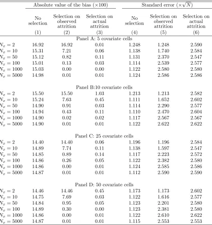
the number of observations per cell. Note that the case withNx= 2 corresponds to pairwise stratification.
In this case, as expect, the bias of the naive estimator (column 1) is the same as the bias of the estimator
that considers only pairs with no realized attrition (column 2). In contrast, the infeasible estimator that
considers only pairs with zero probability of attrition (column 3) would have zero bias. AsNxincreases, the
bias of the estimator that discards covariate cells with realized attrition converge to zero, while the naive
estimator remains biased. We find the same pattern for the cases with differentG(Panels B to D of Table 1). The only difference is that, with more covariate cells, we need a higher total number of observations
N =Nx×Gso that the bias of the estimator that excludes cells with attrition converges to zero.
We also present in columns 4 to 6 the standard error of these estimator (multiplied by√N). As expected, the standard error of the infeasible estimator is always higher than the standard error of the naive estimator,
because the infeasible estimator relies on fewer observations. While the standard error of the estimator that
excludes covariate cells with observed attrition starts at the same level as the standard error of the naive
estimator, its variance converges to the variance of the infeasible estimator whenNx→ ∞. This is consistent
with Proposition1, which shows that these two estimators are asymptotically equivalent. The main intuition
is that one would discard cells with positive probability of attrition with probability approaching to one.
3.2
MC: Selecting cells with no differential attrition
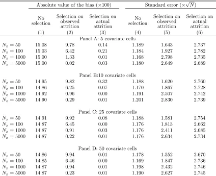
We now modify the DGP used in Section 3.1 so that all covariate cells have some positive probability
of attrition, although for some covariate cells there is no differential probability of attrition. We add a
10% probability that any observation would not be selected, independently of X∗
i and Yi. We keep all
other parameters the same as the ones in Section 3.1. In this case, observations in the bottom 20% of
the distribution ofX∗
i have a 10% probability of attrition irrespectively of treatment status, so there is no
differential attrition, while for largerX∗
i we have a higher probability of attrition for treated observations,
so we have differential attrition. The results, presented in Table 2, are similar to the ones presented in
Section 3.1. With few observations, the bias of the estimator that selects covariate cells with no observed
differential attrition is close to the bias of the naive estimator, but it converges to zero when Nx → ∞.6
The only difference is that, conditional onG, we require a much largerNx so that the bias is close to zero
when compared to the results in Section 3.1. This happens because, for a given Nx, we have much more
power to reject the null if we define that a cell has attrition problem when even only one individual is not
selected. However, the problem with this approach is that we may end up discarding more observations
6
than necessary. Under assumption2, we could have covariate cells that could be used for point estimation
even if there is some positive probability of attrition. Indeed, under this DGP, note that we would end up
discarding all covariate cells with probability approaching to one if we used the strategy from Section3.1to
select covariate cells.
3.3
MC: Selecting cells with lower attrition rates to construct bounds
Finally, we consider the strategy proposed in Section 2.3. We use the same parameters we considered in
Section3.1, but we change the distribution ofX∗, so that it is easier to present the main mechanisms that
lead to distortions when one selects covariate cells based on the observed attrition. We consider now that we
have one covariate cell withX∗= 0.4 (which implies a 10% probability of attrition for treated observations)
andG−1 covariate cells withX∗= 0.8 (which implies a 30% probability of attrition for treated observations).
In this DGP, there is only positive probability of attrition for treated observations, so the potential finite
sample problem raised in Lee(2009) that the estimated differential attrition might lead the researcher to
trim the “wrong” group with a nontrivial probability is absent in this case. Therefore, we can focus solely
on the finite sample distortions generated by the strategy of selecting covariate cells based on the observed
attrition rates. For each replication, we first calculate the Lee bounds using the entire sample. Then we
restrict the sample to covariate cells withobserved differential attrition lower than 25%.7 Finally, we consider
an infeasible estimator in which we restrict to covariate cells with populational differential attrition lower
than 25%. Note that, since we consider a DGP with homogeneous treatment effects, in the three cases we
provide bounds to the same parameter.
For these three bounds’ estimators, we construct confidence intervals for the parameter of interest based
on Imbens and Manski (2004). We present empirical coverage rates in columns 1 to 3 of Table 3. When
we consider the Lee bounds for the entire sample (column 1) and when we select on the covariate cell with
lower probability of attrition (column 3), we have a coverage rate of around 95%, regardless of the number
of observations per covariate cell. When we select covariate cells with observed differential attrition lower
than 25%, however, we have undercoverage when the number of observations per covariate cells is not large.
With 5 covariate cells (4 of which should be discarded), we get an empirical coverage rate of around 90%
when Nx = 50, although it gets close to 95% when Nx = 1000 (panel A of Table 3). The undercoverage
problem becomes more severe when we have more covariate cells. With 50 covariate cells, we have an
7
empirical coverage of only 30% when Nx = 50 (panel A of Table3). With Nx = 5000, however, we have
again a coverage rate of around 95%, which is consistent with Proposition3. The intuition for this result
is that, with more covariate cells that should be discarded, there is a higher probability that we would end
up with at least one of these covariate cells with observed differential attrition sufficiently lower than its
population differential attrition rates. Therefore, one should worry about coverage distortions using our
strategy of selecting cells with relatively lower differential attrition when there are many covariate cells with
few observations each to decide which ones should be discarded.
We also present in columns 4 to 6 of Table3width of the confidence intervals for these three estimators.
WhenNx is small and we have many covariate cells, the width of the confidence interval of the infeasible
estimator that selects only the covariate cell with lower differential attrition islarger than the width of the
confidence interval using all covariate cells. This happens because, while the population bounds when we
consider only the covariate cell with lower differential attrition is tighter, we estimate these bounds using
fewer observations. In this case, the larger standard errors of the bounds’ estimators end up leading to larger
confidence intervals. When Nx increases, the reduction in sample size when we consider only a subset of
the covariate cells becomes less relevant, so with large Nx the strategy of selecting only the covariate cell
with lower differential attrition leads to tighter confidence intervals. Note that the width of the confidence
intervals when we select covariate cells based on the observed attrition is lower relative to the case in which
we use all observations, even whenNxis small. However, this happens because we end up selecting covariate
cells that should not be selected, which ends up generating undercoverage. WhenNx increases, the width of
the confidence intervals when we select covariate cells based on the observed and on the actual differential
attrition becomes very similar, which is consistent with Proposition3.
Finally, we consider in Table4 results when we use covariateX to tighten the bounds as derived inLee
(2009), both when we use all covariate cells and when we select covariate cells based on observed attrition
rates. Note that we still have important gains in terms of tighter confidence intervals when we select covariate
cells with lower attrition rates whenNxis large. The main difference relative to the previous case is that now
we have some undercoverage whenNx is small, even when we use all covariate cells (column 1). However,
the undercoverage we get when we select covariate cells based on observed attrition rates is always more
severe.
Overall, these results suggest that a strategy of selecting covariate cells with lower observed differential
attrition rates may not be attractive when the number of observations per covariate cell is small, as this
covariate cells is large, however, the loss in precision becomes negligible and the bias goes to zero, so this
strategy may lead to more informative results, even if only for the average treatment effect for a well-defined
subpopulation.
4
Empirical Application
We derived in Section2.3a partial identification strategies that may generate more informative bounds by
selecting covariate cells with lower attrition problems. MC simulations presented in Section3.3illustrate the
potential benefits of this strategy in terms of providing tighter bounds when the number of observations per
covariate cell is large, and also potential pitfalls when there are only few observations per covariate cell. In
this section, we consider the use of this strategy in a real application. More specifically, we revisitLee(2009)
study on the impacts on wages of the The Job Corps program, an education and job-training intervention
in the U.S.8. The Job Corps program is federally funded and organized by the US department of Labor
and focuses on disadvantaged youths aged 16 to 24 years old. A participant usually received vocational
and academic training among many other benefits such as room, board, and health services. The program
typically lasts for eight months, and participants were randomly selected.9 The selection problem arises on
evaluating the impact of the program on wage. We only observe wage from individuals who are employed
and it is expected that the program also affected the likelihood of finding a job. Therefore, it is not possible
to correctly assess the average impact of the program on wage by simply comparing the average wages of
treated and non-treated individuals. It is very well likely that employed treated individuals have different
non-observable characteristics than employed non-treated individuals.
Lee(2009) estimates bounds for the parameter of interest under assumption2. He estimates the impact
four years after the end of the program. The overall differential attrition between treatment and control
group is 6.8%. In the main specification without control variables, the usual trimming procedures find 0.093
(-0.019) as the the upper (lower) bound of the treatment effect. In order to tighten the bounds, Lee also
calculates the bounds for different cells based on covariates, and then, estimate bounds for the average
(weighted) effect of the treatment. Lee calculates the projection of wage on several socio-demographics
and uses the quartiles of the wage fitted value to create four different cells. The estimated average lower
and upper bounds are -0.012 and 0.089, respectively. Although, this procedure generates tighter bounds
8
Other papers have evaluated different effects of the Job Corps intervention; see, for instance,Flores et al.(2012), FLORES-LAGUNES et al.(2010) andFrumento et al.(2012).
9
compared to the main specification, the gain is not very large.
We consider the same dataset as Lee and create four cells based on gender and age (above and under
20 years old). The main idea is that differential attrition can potentially be related to covariate groups
and, if there is a set of covariate cells with lower differential attrition, then it might be possible to estimate
tighter bounds for this subpopulation. Table 5 depicts the proportion of selection in each cell. In all but
one, the differential attrition rates hinge around 9%. The group of young male present the smallest level of
differential attrition with px(0)−px(1)
px(0) just below 2%. The table also shows the number of selected observation
in each cell. It is important to notice that there are many observations per covariate cell, and that we are
considering only four covariate cells so, in light of our results from Section3.3, it is unlikely that confidence
intervals based on our strategy would generate undercoverage.
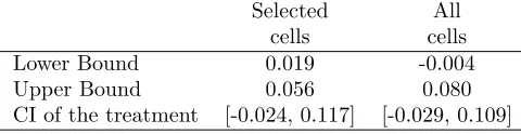
We then estimate the bounds for the only cell with px(0)−px(1)
px(0) below 5% (young males). Table5compares
the results of this exercise with the ones from Lee’s original procedure using the same set of covariates.
Considering the point estimates for the upper and lower bounds, we are able to achieve substantially tighter
bounds relative to the case in which we consider all covariate cells. When we consider the standard errors
of the bounds’ estimators, however, then confidence intervals using both strategies have roughly the same
width.10 This happens because we have to discard many observations from covariate cells with higher
differential attrition rates, so we get less precise estimators for the bounds, as discussed in Section 3.3.
Importantly, we should expect that the strategy of selecting only this covariate cell with lower attrition
would lead to tighter confidence intervals if we had a bigger sample size.
As discussed before, it is important to bear in mind that this strategy compromises external validity. This
may be specially critical in the Job Corp program evaluation. Schochet et al.(2008) have shown important
heterogenous effects of the program for different demographic groups. More specifically, they have shown
that young adults (20-24 years old) experienced larger impacts on weekly earnings compared to adolescents
(16-19 years old). Blanco et al. (2013a) andBlanco et al. (2013b) taking into consideration the potential
sample selection also find larger impacts on wages for young adults compared to adolescents. However, while
this strategy compromises external validity, it may be more informative for well-defined subgroups.
10
5
Concluding Remarks
Sample attrition may invalidate even well implemented field experiments. Given that existing solutions to
deal with attrition may rely on strong assumptions and/or lead to uninformative bounds, researchers might
be tempted to consider subsamples in which attrition problems are more mild. We show that strategies
of selecting subsamples based on observed attrition rates are asymptotically valid when the number of
observations per covariate cell goes to infinity. However, in finite sample such strategies may lead to important
distortions as there might be a nontrivial probability that a covariate cell with severe probabilities of attrition
in the population turns out to have low observed attrition rates in a given sample. In this case, the fact that
one does not discard this covariate cell could be correlated with potential outcomes, leading to inconsistent
estimators.
Importantly, the validity of the strategies we propose relies on the fact that covariate cells are selected
based on pre-determined rules, depending on their observed attrition rates. However, in real applications it
is possible that researchers try different rules to select covariate cells, and this may lead to opportunities to
choose specific rules that lead to significant results, a problem that has received increasing attention in social
sciences.11 Such potential problem highlights the importance of pre-analysis plans in randomized control
trials, in which a researcher could define ex-ante which variables and which rules would be used to select
covariate cells in case of attrition.12 By committing to a given set of rules that a researcher would be allowed
to use to select covariate cells to deal with attrition this specification searching problem would be mitigated.
11
SeeChristensen and Miguel(2016) for a recent survey on transparency in economics research.
12
References
Ahn, Hyungtaik and James L. Powell, “Semiparametric estimation of censored selection models with
a nonparametric selection mechanism,”Journal of Econometrics, 1993,58(1), 3 – 29.
Andrews, Donald W. K. and Marcia M. A. Schafgans, “Semiparametric Estimation of the Intercept
of a Sample Selection Model,”The Review of Economic Studies, 1998, 65(3), 497–517.
Blanco, German, Carlos A. Flores, and Alfonso Flores-Lagunes, “Bounds on Average and Quantile
Treatment Effects of Job Corps Training on Wages,”Journal of Human Resources, 2013,48(3), 659–701.
, , and , “The Effects of Job Corps Training on Wages of Adolescents and Young Adults,” The
American Economic Review, 2013, 103(3), 418–422.
Bruhn, Miriam and David McKenzie, “In Pursuit of Balance: Randomization in Practice in
Develop-ment Field ExperiDevelop-ments,”American Economic Journal: Applied Economics, October 2009,1(4), 200–232.
Christensen, Garret and Edward Miguel, “Transparency, Reproducibility, and the Credibility of
Eco-nomics Research,” Technical Report dec 2016.
Coffman, Lucas C. and Muriel Niederle, “Pre-analysis Plans Have Limited Upside, Especially Where
Replications Are Feasible,”Journal of Economic Perspectives, 2015,29 (3), 81–98.
Das, Mitali, Whitney K. Newey, and Francis Vella, “Nonparametric Estimation of Sample Selection
Models,”The Review of Economic Studies, 2003, 70(1), 33–58.
Flores, Carlos A., Alfonso Flores-Lagunes, Arturo Gonzalez, and Todd C. Neumann,
“Estimat-ing the Effects of Length of Exposure to Instruction in a Train“Estimat-ing Program: The Case of Job Corps,”The
Review of Economics and Statistics, 2012, 94(1), 153–171.
FLORES-LAGUNES, ALFONSO, ARTURO GONZALEZ, and TODD NEUMANN,
“LEARN-ING BUT NOT EARN“LEARN-ING? THE IMPACT OF JOB CORPS TRAIN“LEARN-ING ON HISPANIC YOUTH,”
Economic Inquiry, 2010,48 (3), 651–667.
Frumento, Paolo, Fabrizia Mealli, Barbara Pacini, and Donald B. Rubin, “Evaluating the Effect
of Training on Wages in the Presence of Noncompliance, Nonemployment, and Missing Outcome Data,”
Heckman, James, “Varieties of Selection Bias,”The American Economic Review, 1990, 80(2), 313–318.
Heckman, James J., “Sample Selection Bias as a Specification Error,”Econometrica, 1979,47(1), 153–
161.
Horowitz, Joel L. and Charles F. Manski, “Nonparametric Analysis of Randomized Experiments with
Missing Covariate and Outcome Data,”Journal of the American Statistical Association, 2000, 95 (449),
77–84.
Imbens, Guido W. and Charles F. Manski, “Confidence Intervals for Partially Identified Parameters,”
Econometrica, 2004,72(6), 1845–1857.
King, Gary, Emmanuela Gakidou, Nirmala Ravishankar, Ryan T. Moore, Jason Lakin, Manett
Vargas, Martha Mar´ıa T´ellez-Rojo, Juan Eugenio Hern´andez ´Avila, Mauricio Hern´andez
´
Avila, and H´ector Hern´andez Llamas, “A ”Politically Robust” Experimental Design for Public
Policy Evaluation, with Application to the Mexican Universal Health Insurance Program,” Journal of
Policy Analysis and Management, 2007,26, 479–506.
Lee, David S., “Training, Wages, and Sample Selection: Estimating Sharp Bounds on Treatment Effects,”
The Review of Economic Studies, 2009,76 (3), 1071.
Olken, Benjamin A., “Promises and Perils of Pre-analysis Plans,”Journal of Economic Perspectives, 2015,
29(3), 61–80.
Rubin, Donald B., “Inference and missing data,”Biometrika, 1976,63 (3), 581.
Schochet, Peter Z., John Burghardt, and Sheena McConnell, “Does Job Corps Work? Impact
Findings from the National Job Corps Study,”American Economic Review, December 2008,98(5), 1864–
86.
Zhang, Junni L. and Donald B. Rubin, “Estimation of Causal Effects via Principal Stratification When
Some Outcomes are Truncated by ?Death?,” Journal of Educational and Behavioral Statistics, 2003, 28
Table 1: Selecting cells with no attrition - bias and standard error
Absolute value of the bias (×100) Standard error (×√N)
No selection
Selection on observed attrition
Selection on actual attrition
No selection
Selection on observed attrition
Selection on actual attrition
(1) (2) (3) (4) (5) (6)
Panel A: 5 covariate cells
Nx= 2 16.92 16.92 0.01 1.248 1.248 2.590
Nx= 10 15.31 7.21 0.06 1.138 1.740 2.584
Nx= 50 15.12 0.82 0.11 1.131 2.370 2.547
Nx= 100 15.01 0.13 0.03 1.114 2.539 2.577
Nx= 1000 15.03 0.00 0.00 1.122 2.580 2.580
Nx= 5000 14.98 0.01 0.01 1.124 2.586 2.586
Panel B:10 covariate cells
Nx= 2 15.50 15.50 1.03 1.213 1.213 2.582
Nx= 10 15.24 7.63 0.45 1.111 1.652 2.602
Nx= 50 14.90 0.91 0.03 1.114 2.290 2.577
Nx= 100 14.94 0.43 0.11 1.110 2.470 2.604
Nx= 1000 14.90 0.02 0.02 1.117 2.567 2.567
Nx= 5000 14.90 0.01 0.01 1.122 2.622 2.622
Panel C: 25 covariate cells
Nx= 2 14.40 14.40 0.06 1.196 1.196 2.584
Nx= 10 14.89 7.74 0.11 1.138 1.597 2.547
Nx= 50 14.85 0.89 0.14 1.117 2.223 2.572
Nx= 100 14.86 0.26 0.05 1.122 2.382 2.580
Nx= 1000 14.86 0.00 0.01 1.124 2.585 2.586
Nx= 5000 14.87 0.01 0.01 1.112 2.590 2.590
Panel D: 50 covariate cells
Nx= 2 14.46 14.46 0.45 1.173 1.173 2.602
Nx= 10 14.75 7.69 0.03 1.122 1.616 2.577
Nx= 50 14.84 0.95 0.05 1.123 2.201 2.580
Nx= 100 14.89 0.30 0.00 1.123 2.381 2.580
Nx= 1000 14.86 0.00 0.01 1.122 2.610 2.622
Nx= 5000 14.87 0.01 0.01 1.115 2.553 2.553
Table 2: Selecting cells with no differential attrition - bias and standard error
Absolute value of the bias (×100) Standard error (×√N)
No selection
Selection on observed attrition
Selection on actual attrition
No selection
Selection on observed attrition
Selection on actual attrition
(1) (2) (3) (4) (5) (6)
Panel A: 5 covariate cells
Nx= 50 15.08 9.78 0.14 1.189 1.643 2.737
Nx= 100 15.03 6.42 0.21 1.184 1.927 2.782
Nx= 1000 15.00 1.33 0.01 1.168 2.798 2.735
Nx= 5000 15.00 0.02 0.03 1.180 2.649 2.689
Panel B:10 covariate cells
Nx= 50 14.95 9.82 0.32 1.188 1.620 2.760
Nx= 100 14.86 6.25 0.07 1.170 1.867 2.728
Nx= 1000 14.92 0.96 0.00 1.191 2.507 2.742
Nx= 5000 14.90 0.29 0.01 1.201 2.830 2.739
Panel C: 25 covariate cells
Nx= 50 14.91 9.92 0.08 1.188 1.581 2.754
Nx= 100 14.87 6.45 0.00 1.176 1.813 2.662
Nx= 1000 14.87 0.91 0.03 1.176 2.411 2.685
Nx= 5000 14.87 0.22 0.01 1.176 2.634 2.734
Panel D: 50 covariate cells
Nx= 50 14.86 9.94 0.01 1.178 1.552 2.670
Nx= 100 14.85 6.46 0.00 1.169 1.847 2.736
Nx= 1000 14.87 0.94 0.01 1.198 2.432 2.746
Nx= 5000 14.87 0.23 0.01 1.190 2.627 2.745
Table 3: Lee bounds selecting cells with lower differential attrition (without covariates to tighten bounds)
Empirical coverage Width of the confidence interval
No selection
Selection on observed attrition
Selection on actual attrition
No selection
Selection on observed attrition
Selection on actual attrition
(1) (2) (3) (4) (5) (6)
Panel A: 5 covariate cells
Nx= 50 0.958 0.905 0.955 0.819 0.737 0.803
Nx= 100 0.954 0.904 0.946 0.736 0.624 0.611
Nx= 1000 0.955 0.943 0.947 0.600 0.334 0.330
Nx= 5000 0.960 0.952 0.952 0.566 0.258 0.258
Panel B:10 covariate cells
Nx= 50 0.955 0.829 0.955 0.767 0.677 0.803
Nx= 100 0.951 0.838 0.945 0.710 0.616 0.611
Nx= 1000 0.954 0.938 0.947 0.614 0.338 0.330
Nx= 5000 0.952 0.951 0.951 0.590 0.258 0.258
Panel C: 25 covariate cells
Nx= 50 0.954 0.601 0.955 0.712 0.591 0.803
Nx= 100 0.952 0.635 0.946 0.676 0.577 0.611
Nx= 1000 0.951 0.920 0.947 0.616 0.353 0.330
Nx= 5000 0.951 0.953 0.953 0.601 0.258 0.258
Panel D: 50 covariate cells
Nx= 50 0.953 0.301 0.955 0.682 0.539 0.804
Nx= 100 0.955 0.343 0.946 0.656 0.541 0.611
Nx= 1000 0.951 0.892 0.948 0.614 0.374 0.330
Nx= 5000 0.951 0.952 0.952 0.603 0.258 0.258
Table 4: Lee bounds selecting cells with lower differential attrition (with covariates to tighten bounds)
Empirical coverage Width of the confidence interval
No selection
Selection on observed attrition
Selection on actual attrition
No selection
Selection on observed attrition
Selection on actual attrition
(1) (2) (3) (4) (5) (6)
Panel A: 5 covariate cells
Nx= 50 0.933 0.886 0.955 0.745 0.698 0.803
Nx= 100 0.935 0.890 0.946 0.679 0.596 0.611
Nx= 1000 0.947 0.942 0.947 0.562 0.333 0.330
Nx= 5000 0.953 0.952 0.952 0.530 0.258 0.258
Panel B:10 covariate cells
Nx= 50 0.911 0.790 0.955 0.704 0.634 0.803
Nx= 100 0.920 0.812 0.945 0.667 0.580 0.611
Nx= 1000 0.944 0.936 0.947 0.592 0.336 0.330
Nx= 5000 0.946 0.951 0.951 0.569 0.258 0.258
Panel C: 25 covariate cells
Nx= 50 0.858 0.518 0.955 0.659 0.558 0.803
Nx= 100 0.895 0.580 0.946 0.645 0.547 0.611
Nx= 1000 0.934 0.915 0.947 0.605 0.346 0.330
Nx= 5000 0.944 0.953 0.953 0.592 0.258 0.258
Panel D: 50 covariate cells
Nx= 50 0.786 0.212 0.955 0.632 0.512 0.804
Nx= 100 0.856 0.283 0.946 0.629 0.519 0.611
Nx= 1000 0.927 0.882 0.948 0.607 0.362 0.330
Nx= 5000 0.940 0.952 0.952 0.598 0.258 0.258
Table 5: Empirical application: sample selection by covariate cell
% Selection
Cells px(1) px(0) px(1)px−(1)px(0) N
Male Old 0.732 0.662 0.093 918
Young 0.587 0.576 0.019 2210
Female Old 0.641 0.589 0.088 776
Young 0.564 0.508 0.098 1523
Notes: “Old” means twenty years of age or older; “Young” means younger than twenty years. px(1) and
px(0) are the proportion of employed individuals in the
treatment and control groups, respectively. N is the number of observations.
Table 6: Empirical application: bounds’ estima-tors
Selected All
cells cells
Lower Bound 0.019 -0.004
Upper Bound 0.056 0.080
CI of the treatment [-0.024, 0.117] [-0.029, 0.109] Notes: “Selected cells” group includes only cells with differential selection below 5% (young males); “All cells” group includes all cells regardless the differential attri-tion. Lower and Upper bounds are calculated based on
Lee(2009). For the “All cells” group estimation, gender and age dummies were used to tighten the bounds. CI of treatment is calculated based onImbens and Manski
[image:27.612.185.425.318.380.2]A
Appendix
A.1
Proof of Proposition
1
Assume that the number of observations in covariate cell xis given by Nx =f(x)N for allN. Then the
estimator ˆτ can be written as:
ˆ
τ= PG 1
x=11{x∈Γˆ}f(x)
G
X
x=1
1{x∈Γˆ}f(x)ˆτx (12)
From equation 7, we know that:
1{x∈Γˆ} →p
1 ifx∈Γ
0 ifx /∈Γ
(13)
which implies thatPG
x=11{x∈Γˆ}f(x)→p
PG
x=11{x∈Γ}f(x).
Moreover, we know that√N(ˆτx−τx)→d N
0,f(1x)p(1σ−2p)ifx∈Γ and ˆτx=Op(1) ifx /∈Γ. Therefore:
ˆ
τ →p
1
PG
x=11{x∈Γ}f(x)
G
X
x=1
1{x∈Γ}f(x)τx=
1
P
x∈Γf(x)
X
x∈Γ
f(x)τx=E[τx|x∈Γ] (14)
and:
√
N(ˆτ−E[τx|x∈Γ])→dN 0,
1 (P
x∈Γf(x))2
X
x∈Γ
f(x) σ
2
p(1−p)
!
(15)
A.2
Proof of Proposition
2
For each x, we want to test H0 : |px(1)−px(0)| ≤ ǫ at αsignificance level. Consider the decision rule
such that we reject H0 if either pˆx(1)−σˆpˆx(0)−ǫ >Φ(1−α) or pˆx(1)−ˆσpˆx(0)+ǫ <Φ(α), where ˆσ is a consistent
estimator for the standard error of ˆpx(1)−pˆx(0) and Φ(.) is the CDF of the standard normal. Note that, for
any px(1)−px(0) such that|px(1)−px(0)| ≤ǫ, we have that P r(reject H0|px(1)−px(0))→α˜ ≤αwhen
Nx → ∞. For example, if px(1)−px(0) = ǫ, then P r
pˆ
x(1)−pˆx(0)−ǫ
ˆ
σ >Φ(1−α)|px(1)−px(0) =ǫ
→ α
while P rpˆx(1)−pˆx(0)+ǫ
ˆ
σ <Φ(α)|px(1)−px(0) =ǫ
→0. The opposite happens when px(1)−px(0) = −ǫ.
As in proposition 1, we have that:
ˆ
τ′=
PG
x=11{x∈Γˆ′}[p(1−pˆx(1)) + (1−p)(1−pˆx(0))]f(x)ˆτx
PG
x=11{x∈Γˆ′}[p(1−pˆx(1)) + (1−p)(1−pˆx(0))]f(x)
(16)
Since we assume that|px(1)−px(0)|> ǫforx /∈Γ′, we have that:
1{x∈ˆΓ′} →
p
1 ifx∈Γ′
0 ifx /∈Γ′
(17)
Moreover, for x∈Γ′, we have that ˆp
x(1)→ppx, ˆpx(0)→ppx, and √
N(ˆτx−τx)→dN
0, 1
pxf(x)
σ2
p(1−p)
.
Also, ˆτx=Op(1) ifx /∈Γ′. Therefore:
ˆ
τ′ →p
1
PG
x=11{x∈Γ′}pxf(x) G
X
x=1
1{x∈Γ′}pxf(x)τx=
1
P
x∈Γ′pxf(x)
X
x∈Γ′
pxf(x)τx=τ′ (18)
and:
√
N(ˆτ−τ′)→dN 0, 1
(P
x∈Γpxf(x))2
X
x∈Γ
pxf(x) σ
2
p(1−p)
!