Munich Personal RePEc Archive
Framing Effects in Intertemporal Choice:
A Nudge Experiment
Faralla, Valeria and Novarese, Marco and Ardizzone,
Antonella
Dipartimento di Giurisprudenza e Scienze Politiche, Economiche e
Sociali, Università del Piemonte Orientale, Dipartimento di
Giurisprudenza e Scienze Politiche, Economiche e Sociali, Università
del Piemonte Orientale, Dipartimento di Economia, Studi Giuridici e
Aziendali, Università IULM
September 2017
Online at
https://mpra.ub.uni-muenchen.de/82086/
1
Framing Effects in Intertemporal Choice: A Nudge Experiment
By Valeria Farallaa, Marco Novaresea, and Antonella Ardizzoneb
Preprint version
published in the Journal of Behavioural and Experimental Economics (/1) 2017 13-25
a
Dipartimento di Giurisprudenza e Scienze Politiche, Economiche e Sociali, Università del Piemonte Orientale, Palazzo Borsalino, Via Cavour 84, 15121 Alessandria, Italy,
valeria.faralla@uniupo.it, marco.novarese@uniupo.it
b
Dipartimento di Economia, Studi Giuridici e Aziendali, Università IULM, via Carlo Bo 8, 20143 Milano, Italy, antonella.ardizzone@iulm.it
Corresponding Author:
Valeria Faralla
Dipartimento di Giurisprudenza e Scienze Politiche, Economiche e Sociali Università del Piemonte Orientale “Amedeo Avogadro”
Palazzo Borsalino, Via Cavour 84 15121 Alessandria (Italy)
Phone: +39-0131-283756
2
ABSTRACT
This paper experimentally investigates the framing effects of intertemporal choice using two different elicitation modes, termed classical and penal. In the classical mode, participants are given the choice between receiving a certain amount of money, smaller and sooner, today and a higher amount, larger and later, delayed (e.g., “€55 today vs. €75 in 61 days”). This is referred to as the standard mode. In the penalty mode, the participant must give up an explicit amount of money in order to choose the smaller and sooner option (e.g., “€75 in 61 days vs. €55 today with a penalty of €20”). This is the explicit mode. We find that estimates of individual discount rates are lower in the explicit mode than in the standard mode. This result suggests that even very simple information about the amount of money one must surrender for choosing the earlier option increases delayed consumption. The finding has relevant implications for self-control and long-term planning in intertemporal choice.
3
1. Introduction
A decision problem is a problem that can be “defined by the acts or options among which one must choose, the possible outcomes or consequences of these acts, and the contingencies or conditional probabilities that relate outcomes to acts” (Tversky and Kahneman, 1981, p. 453). Despite a decision problem can be formulated in different ways, according to standard models of intertemporal (Samuelson, 1937) as well as risky (von Neumann and Morgenstern, 1947) choice, the decision-maker should not be influenced by variations in the framing of options when this variation does not affect the possible outcomes.
Experimental research has shown however that standard rational agent models are not consistent with a wide range of actual individual behaviours (see Frederick, Loewenstein, and O’Donoghue, 2002, for intertemporal choices, and Kahneman, 2012, for risky decisions) and that different elicitation modes, choices with logically equivalent presentations of the same decision problem, affect decision-making processes (e.g., Kahneman and Tversky, 1979; Levin, 1987; Li and Xie, 2006; Li, Sun, and Wang, 2007; Lichtenstein, Burton, and Karson, 1991; Loewenstein and Prelec, 1992; Tversky and Kahneman, 1992). Accordingly, the rational evaluation of an option seems to be affected by its formal presentation (i.e., frame) rather than its final level of wealth. Real-life decisions are indeed highly context-dependent (Simonson and Tversky, 1992), a finding which has been also supported at a neurobiological level (Louie, Khaw, and Glimcher, 2013; Louie and De Martino, 2014). In particular, the framing of decisions is not only due to the formulation of a particular decision problem but also to additional factors such as personality traits or individual habits and people often seem to not be conscious of their cognitive biases (Kahneman, 2012). Nevertheless, the effect of framing holds for real and hypothetical choices and for both non-monetary and non-monetary outcomes (Kahneman, 2012; Mischel and Underwood, 1974; Tversky and Kahneman, 1981; 1986; Wilson and Daly, 2004).
To date, framing effects have been mainly investigated in the context of decision-making under risk. In particular, all other things being equal, individuals have been consistently found to change their preference in the choice between a sure and a risky outcome when the prospects are framed in terms of gains or losses. Specifically, people seem to be risk-averse in the gain frame (i.e., a certain gain or the probability of winning an amount of money versus the complementary probability to winning nothing) but risk-seeking in the loss one (i.e., a certain loss or the probability of losing an amount of money versus the complementary probability to losing nothing) (Tversky and
4
account the fact that people are not perfectly rational nor have complete knowledge and unlimited cognitive abilities, as described in classical economic theory (von Neumann and Morgenstern, 1947).
According to Kahneman and Tversky’s theory, the decision-making process can be divided into two different steps, namely the framing phase and the evaluation phase. In the framing phase, which is prior to the evaluation one, the decision-maker selects the part of the information which considers important for the choice. Then, in the evaluation phase, the individual assesses the value of the decision problem and finally makes the choice. As a result, framing affects the evaluation of an option by subjectively determining the features that are relevant for the subsequent choice and this is typically established through a reference point, an outcome which is considered as neutral and from which possible outcomes are perceived as positive or negative deviations (and then as a gain or a loss, respectively). In prospect theory, the value of a prospect is indeed defined in changes rather than final states of wealth. Returning to the example above (Tversky and Kahneman, 1981), when a decision problem is framed in terms of losses, the reference point is that of having
something to lose and the opportunity to play the gamble, rather than opting for the certain loss, is considered as a positive deviation (sure losses are in fact particularly aversive). This is just the opposite in the gain frame. In line with experimental evidence, this implies risk-aversion behaviour for gains and risk-seeking choices for losses and indeed the individual value function, which is defined on deviations from the reference point, is typically concave for gains and convex for losses (see original work for details on theoretical and modeling analysis (Kahneman and Tversky, 1979 and Tversky and Kahneman, 1992)).
The framing effect in risky choice is not limited to the domain of money and it has been also found using non-monetary options and in non-humans. For instance, McNeil et al. (1982) observed that surgery was more often chosen by using survival, rather than mortality, rate frames (i.e., “the one-month survival rate is 90%” versus “there is 10% mortality in the first month”). Tversky and Kahneman (1981) showed that framing a choice in terms of “lives saved” seems to induce aversion, whereas the decision problem described in terms of “lives lost” tends to increase risk-seeking behaviours. More recently, Chen, Lakshminarayanan, and Santos (2006) found capuchin monkeys’ preference for gain-framed rather than loss-framed gambles, suggesting a possible evolutionary explanation for framing.
5
et al., 2007; for interesting background information, see Elliott and Hayward, 1998). Again, people appear to represent future payoffs as gains or losses from a reference point, but also past or future consumption and even others’ choices (Loewenstein, 1988; see also, for instance, Epley and Gneezy, 2007).
In intertemporal choice, the most common experimental decision task is to submit choices between receiving a certain amount of money, Smaller and Sooner (SS), today (or in the short term) and a higher amount, Larger and Later (LL), delayed (e.g., “$34 tonight or $35 in 43 days”; Kirby and Maraković, 1996). This is a choice between two outcomes represented by different sizes and available for delivery at two different points in time which can be considered as a standard format of decision problems for eliciting discount rates— a measure of the steepness at which individuals discount future rewards over immediate ones, from individual choice (Hardisty and Weber, 2009; Kirby, 1997; Kirby, Petry, and Bickel, 1999; Weber et al., 2007; Zauberman et al., 2009). The individual discount rate is considered as a proxy of the individual impulsiveness according to which higher rates correspond to an increasing choice of the sooner than later reward. In fact, people consider as less valuable the present value of future rewards as the delay at which the reward is available increases and then tend to discount future rewards as a function of delay—that is known as delay (or temporal) discounting.
Decision problems have been represented, however, in different forms and framing effects have been found to be involved in the elicitation of discount rates according to the particular format chosen. For example, Read and Roelofsma (2003) focused on the difference between standard choices and matching modes, framings in which participants are required to state a particular value that equal two different options according to their preferences (e.g., “£???? Sept 28, 2001 or £1000 Sept 27, 2002”). They found increasing discount rates associated with delay, especially in the matching frame. Although the difference was not so pronounced, this finding is in line with
previous research comparing these two conditions (see also Ahlbrecht and Weber, 1997; Breuer and Soypak, 2015; Malkoc and Zauberman, 2006).
6
In line with these findings, as was observed for the standard model of decision-making under risk, the normative theory of intertemporal choice has been criticized in favour of more descriptive models of discounting future events, especially hyperbolic (Ainslie, 1992; 2001) but also quasi-hyperbolic (Elster, 1979; Laibson, 1997; Phelps and Pollak, 1968), sub-additive (Read and Roelofsma, 2003), additive-utility (Killeen, 2009), or interval discounting (Scholten and Read, 2006). Specific models of framing have been also proposed (Loewenstein, 1987; Loewenstein and Prelec, 1992; Read et al., 2005). For instance, Loewenstein (1987) incorporated the concept of reference point into the intertemporal choice model and showed that people tend to be more impatient when the options are expressed in terms of delay rather than speed-up (acceleration) forms in which the future reward is anticipated (i.e., keep a $7 gift certificate available at an
appointed time versus trading the same certificate for a smaller, earlier one). A similar situation was more recently investigated by Weber et al. (2007). In their study, again, subjects increased their discount rates when decision problems were framed in terms of delay (e.g., “receive a $50 Amazon gift certificate that day” versus “receive a gift certificate of larger value in 3 months”) rather than in terms of speed-up (e.g., “receive a $75 Amazon gift certificate in 3 months” versus “receive a gift certificate of lesser value that day”). According to Loewenstein (1988), these shifts of preference are due to changes in the reference point. More specifically, since in speed-up modes the delayed option seems to be framed as the default option (which is instead represented by the immediate one in delay frames), subjects tend to increase their choice for the delayed reward. Reference points can be induced by factors as reward proximity or anticipate consumption (e.g., for dieters: eat a caloric food now, rather than later; see Ruderman, 1986), which may increase the feeling of deprivation and stimulate impulsive behaviour.
Please note that individuals may be aware that their preferences are subject to contextual influences. Because of this, if they are sufficiently sophisticated, they would behave as rational economic individuals and provide more analytical evaluation of decision problems in both risky and intertemporal choice. Particularly, in intertemporal choice, people may apply pre-commitment strategies (i.e., commit in advance to a certain plan of action, such as using deadlines for task completion; see for instance Ariely and Wertenbroch, 2002) to increase their future orientation, an effort which typically requires self-control (Baumeister, 2002; Houben and Jansen, 2011), and objectivity in individual decision-making. By reducing the difference between objective and subjective components of choice, models of non-standard preferences become more compatible with classical theory (O’Donoghue and Rabin, 2001; Pollak, 1968; Strotz, 1955-56).
7
the failure of descriptive invariance of preference in risky choice and the importance of prospect theory as a more descriptive model of decision-making under risk. As a result, if experimental literature on intertemporal choice is overwhelmingly critical about the use of rational agent models in real life decisions and agrees with the link between elicitation effects and shift of preferences, framing effects in intertemporal choice need to be further investigated, theoretically and
experimentally. Consider, for instance, the importance and implications of framing effects for intertemporal choices and long-term goals in areas such as retirement, energy consumption, or health (Laibson, Repetto, and Tobacman, 1998; Weber, 2004; 2006).
Accordingly, the main aim of this paper is to experimentally investigate the effect of elicitation modes in intertemporal choice by using decision frames where the difference between the SS and paired LL option is explicitly indicated to the participants in each decision problem that we called an explicit penalty decision problem (e.g., “€75 in 61 days vs. €55 today with a penalty of €20”). Decision problems with an explicit penalty will be used and compared to standard modes (e.g., “€55 today vs. €75 in 61 days”). By using this paradigm, we hypothesise that, by giving test subjects simple information about the amount of money the participant has to give up for choosing the smaller and sooner option, individuals tend to shift their preferences in favour of the LL option, and then increase their tendency to be more future-oriented. Specifically, we speculate that the explicit penalty may act as a nudge; that is, an indirect suggestion influencing decision-making without coercive measures (Thaler and Sunstein, 2008), that leads individuals to be more far-sighted. Successful long-term planning has been found to be connected with the ability to anticipate future events, by foreseeing the pleasure/pain connected with possible future events, and, at the same time, to resist immediate or short-term temptations. Anticipation and self-control, together with
representation, are indeed three key features of intertemporal choice which interact each other through mechanisms (already identified and new ones) that are presently only partially explained (Berns, Laibson and Loewenstein, 2007). Accordingly, people may reduce their level of impatience throughout attention or other cognitive mechanisms that should be further investigated, possibly by using neurobiological data in an interdisciplinary approach. Here, we do not intend to present a new mechanism of choice but rather to shown how people can be gently pushed into far-sighted
decisions by making explicit simple information (and then slightly changing their perspective), in accordance with the spirit of nudge.
8
“Would you prefer to receive $700 now or invest it for 1 year for an additional $42?”. To date, however, very similar modes to penalty in intertemporal choice are speed-up modes (e.g., as seen above, “receive a $75 Amazon gift certificate in 3 months” versus “receive a gift certificate of lesser value that day”) or decision problem formulations with explicit reference to opportunity costs. Notably, opportunity costs rely on the fact that people have to think about the pleasure associated with the outcome but also consider other alternative resources, items or experiences, that could give them the same pleasure (see Buchanan, 2008; Carmon and Ariely, 2000; Eatwell,
Milgate, and Newman, 1998; Henderson, 2014). As for intertemporal choice, the opportunity cost of time effect was investigated by Zhao et al. (2015). In their paper, they explicitly referred to the opportunity cost of time by using this formulation: “At the expense of one day of studying time, participate in an extracurricular activity for one day tomorrow” versus “At the expense of two days of studying time, participate in an extracurricular activity for two days in a week”. They found that respondents were more likely to choose the LL option when the opportunity cost was hidden (i.e., no reference to opportunity costs), whereas the SS one was the most preferred in the explicit condition. Frederick et al. (2009) also investigated the role of opportunity costs in intertemporal preference but with monetary choices and purchasing decisions, which may have activated different processes of choice, especially if considering the types of goods at stake. Hidden-zero effects (e.g., “$5 today and $0 in 26 days OR $0 today and $6.20 in 26 days”; Magen, Dweck, and Gross (2008)) have been even considered as drawing attention to the opportunity cost of each choice and
encouraging to select the option with the lower opportunity cost (i.e., the more delayed one). In line with this view, this type of framing has found to account for the decrease of impatience in
intertemporal preference.
However, our approach is basically different from both opportunity costs and the other
formulations here identified. As for opportunity costs, firstly, Zhao et al. investigate the opportunity cost of time rather than money. The same authors emphasize the difference between monetary rewards and availability of time, which has not always a positive connotation. Secondly, an opportunity cost is not necessarily considered as an actual loss or penalty and, indeed, opportunity costs may also consider the positive sides, such as pleasure or benefit, associated with giving up a certain outcome. Moreover, in the processing of opportunity costs, stronger inter-individual difference may apply (Frederick et al. 2009; Zhang, Ji, and Li, 2017).
9
least a minimum of numerical computation which is absent in our explicit penalty frame. Indeed, with the type of framing we employed here, individuals are explicitly indicated the amount of money they have to give up in case of preference of the SS option. As a result, in respect to other less explicit modes, results should not be affected by errors, or at least misrepresentations, when evaluating the prospect of choice. Expected utility considerations can indeed be complex for individuals, even when simple calculation is needed (Kahneman, 2012).
10
2. Study 1: Hypothetical decisions
2.1. Methods
A total of 135 undergraduate students (64% females; age range, 19 to 20 years) from the Department of Law, and Political, Economic, and Social Sciences at the University of Piemonte Orientale participated in the experiment by completing an online survey. The survey was available to the students for a duration of 15 days at a link within Moodle, an electronic learning
environment. All participants provided informed consent and were not compensated for their participation in the study.
Participants were presented a series of intertemporal choices between two different monetary options. For each choice, subjects’ preference was elicited by asking participants to choose between a hypothetical immediate option SS, available at time t, and a larger delayed option LL, at time t+1 (e.g., “€8 today vs. €11 in 1 week”). The SS option was the same on all trials (€8), and it was immediately available (t = today). The respective amounts for the LL options were 8.5, 9, 9.5, 10, 10.5, 11, 11.5, 12 Euros. The delay for LL options (t+1) was fixed and indeed it was available after a delay of two weeks in every choice.
Two different questionnaires were prepared. The standard questionnaire contained standard decision problems (“Would you prefer €8 today or €11 in 1 week?”). In the explicit penalty questionnaire, the amount of money the subject has to give up for choosing the SS option was instead explicitly indicated (“Would you prefer €11 in 1 week or €8 today with a penalty of €3?”). Half of participants were then randomly assigned to either standard version or to the explicit penalty mode.
2.2. Results
The percentage of subjects choosing the SS option was higher in the standard version than in the penalty mode. Specifically, there was a difference of 7 percentage points (24% versus 17%) between the two questionnaires and the difference was found to be statistically significant (Fisher exact test, p-value <.01).
A multiple logistic regression analysis (SS vs. LL options as the outcome variable) including gender, reward size and type of questionnaire (standard vs. explicit penalty) as independent
11
(p-value <.01 and <.001, respectively). Results are summarized in Table 1. The power test indicated a power of 0.98 (significance level = 0.05; effect size = 0.15) (Analysis was performed in Ri368 3.2.2, developed by the R Foundation for Statistical Computing (R Core Team, 2015), with the pwr package (Champely, 2017; effect size benchmarks by Cohen, 1988)).
12
3. Study 2: Weak monetary incentives
3.1. Methods
Three experimental sessions were run for a total of 241 undergraduate students (68% females; median age: 22.99, SD: 1.85). Sessions were conducted at the IULM University of Milan,
Department of Law, Economics and Business, and at the University of Siena, Department of Economics and Statistics, between December 2015 and April 2016. All participants provided consent prior to participation.
3.1.1. Protocol
At the beginning of each session, the researcher informed participants that they were
participating in an experiment on individual decision-making and also explained that their responses would remain completely anonymous and at an aggregate level. Then, each subject was
administered a self-report monetary-choice questionnaire, available in pencil-and-paper form, in two versions. Specifically, half of participants were randomly assigned to either the standard version or to the explicit penalty version of the self-administered questionnaire. At the end of the questionnaire, participants were asked to report their age, degree program, and gender.
Each session lasted around 20 minutes and was performed under identical conditions, using the same methods. All subjects participated in only one session of the study.
Some of the participants in each session were randomly selected to receive one of the reward they stated to prefer in the questionnaire. At the end of the session, indeed, one question was randomly chosen to be paid and the selected participants received their reward according to their choice in that chosen question. The selected subjects were paid for the same choice. Immediate payments were paid in cash at the end of the experimental session. For future rewards, instead, subjects were individually met in their classroom at the number of days needed and paid in cash at no transaction cost. Because of this payment scheme, participants were told that they would make each choice as if it was the one they will receive as reward.
3.1.2. The Monetary-Choice Questionnaire
Subjects participated in the experiment by completing the 27-item Monetary-Choice
Questionnaire (MCQ; Kirby, Petry, and Bickel, 1999), a self-administered questionnaire which is typically used in experimental studies to elicit individual discount rates (see, for instance,
13
2015), and which is based on the questionnaire developed by Kirby and Maraković (1996). In the standard version of the MCQ, participants were presented a series of intertemporal choices between two different monetary options. For each choice, subjects’ preference was elicited by asking
participants to choose between an immediate option SS, at time t, and a larger delayed option LL, at time t+1 (e.g., “Would you prefer €55 today or €75 in 61 days?”). The SS option was immediately available (t = today), whereas the delay for LL options (t+1) was between 7 and 186 days. The possible amounts for the SS reward were ranging from 11 to 80 Euros, whereas the respective amounts for the LL options were between 25 and 85 Euros. Participants were requested to select their preferred option by circling an alternative for each choice of the questionnaire.
As noted earlier, a second version of the MCQ was prepared in which the amount of money the subject has to give up for choosing the SS option was explicitly indicated (e.g., “Would you prefer €75 in 61 days or €55 today with a penalty of €20?”). This version was considered as the explicit penalty mode questionnaire.
Following Kirby, Petry, and Bickel (1999), subjects’ discount rates are estimated from their choices throughout the questionnaire by applying the formula V= A/(1+kD), where V is the present value of the delayed amount A at delay D and k is a parameter identifying the discount rate. This formula is of hyperbolic type (Mazur, 1987). As noted earlier, the hyperbolic model is an alternative to the normative model of intertemporal choice that has been found to be more descriptive of
14
All the choices included in the questionnaire are shown in Appendix A. The order of the questions follows that in Kirby, Petry, and Bickel (1999) which was designed to prevent any correlation between SS and LL options in terms of amounts, ratios, differences, delays, or discount rates. The participants were instructed following the instructions in Appendix B, which were adapted from Kirby, Petry, and Bickel (1999). Particularly, they were instructed about what they would be paid, in the standard as well as the explicit penalty framing, if they were selected for the reward payment. For instance, in the explicit penalty frame, this was used to avoid
misunderstandings about the possibility to receive €55-€20=€35 today (rather than €55) in the choice “Would you prefer €75 in 61 days or €55 today with a penalty of €20?”. Prior to beginning the experiment, participants were questioned to make sure they understood the instructions.
3.2. Results
The main objective of the study was the testing of possible elicitation effects in intertemporal choice by using different decision frames. Specifically, we investigated the question whether a penalty effect occurs when the amount of money the individual has to give up in order to choose the more immediate option in the decision problem is explicitly mentioned. We applied a between-participants design in which between-participants were asked to complete the standard monetary-choice questionnaire or, alternatively, the penalty mode.
The analysis was based on individual discount rates which were elicited from the two different monetary-choice questionnaires (i.e., standard and explicit penalty modes), but also covered
subjects’ willingness to choose later options and information related to demographic characteristics of participants. The demographic information was indeed analysed in terms of individual difference variables. Additional attributes of choice options, such as magnitude and delay, and consistency of results were also examined.
15
Table 2 summarizes the main descriptive results and characteristics of the sample by questionnaire.
3.2.1. Demographic information, general data
Participants age ranged from 20 to 31 years old (mean age = 22.99; SD = 1.85). The median age was comparable in the two groups and indeed the median age was 23.09 (SD = 1.98), in the classic MCQ, and 22.88 (SD = 1.71), in the explicit penalty MCQ.
As for gender, 32% of the subjects were males and the rest 68% were females. Specifically, the number of females was higher in the first two sessions (88% vs. 12%, in session one, and 75% vs. 25%, in session two), but lower in the last one (45% vs. 55%). Despite this, the percentage of females was only slightly higher in the explicit penalty mode questionnaire (71%) than in the standard MCQ version (66%) (not significant). Thus, we decided to investigate for potential gender differences in the comparison of the two questionnaires.
The number of standard and explicit penalty questionnaires was also quite similar for each session. The percentage of classical MCQ delivered was indeed 49%, in the first session, and 51%, in the second and third ones. Age was likewise comparable across sessions, since the mean age computed for the three sessions were 25 (SD =0.98), 23 (SD =1.69), and 21 (SD =1.08),
respectively. These results suggest a substantial homogeneity within the three different sessions. As for subjects’ choices, we firstly checked what percentage of participants selected the more immediate option in each of the two questionnaires. As a result, most of subjects preferred the LL rather than the SS option in both modes. However, the percentage of subjects choosing the SS option was higher in the standard version than in the penalty mode of the MCQ and indeed there was a difference of 9 percentage points between the two questionnaires (percentage of SS options: 43%, in the standard MCQ, and 34%, in the explicit penalty mode). The difference between the choice of LL and SS options in the two modes was found to be statistically significant by means of the Fisher exact test (p-value <.001; Table 3). This result suggests that individuals tend to switch towards the more delayed option when the amount of money subjects have to give up is explicitly indicated.
Second, the choice of the SS option was slightly higher for males than females in the explicit penalty monetary-choice questionnaire (38%, for males, and 31%, for females; p-value <.001). The percentage of SS options chosen in the standard questionnaire was instead the same for both
16
problem was higher for females than males. Indeed, females reduced more than males the choice of the SS option in the explicit penalty version of the questionnaire.
Conversely, the choice of SS options was comparable across sessions in the explicit penalty mode, but not in the classical version of the monetary-choice questionnaire. The percentage of SS preferences was indeed between 39% and 45% in the standard MCQ (p-value <.05) and around 33-35% in the explicit penalty MCQ (not significant). The main results of this section are summarized in Table 2.
3.2.2. Discount rates
The individual discount rates were separately calculated for standard and explicit penalty questionnaire, using a tool developed by Kaplan et al. (2014). Due to the number of non-responses, however, it was not possible to compute discount rates for 11 subjects.
Estimates of individual discount rates were lower in the penalty mode than in the standard framing. The mean discount rate was indeed 0.0214 for the standard MCQ and 0.0103 for the explicit penalty mode questionnaire. This result was consistent across the different sessions and gender groups. Results are summarized in Table 2.
The difference between discount rates elicited for individuals responding in the two different questionnaires was found to be significant different by using the Wilcoxon test (p-value <.01; Table 3). This result, which is in line with descriptive data analysis in section 3.1, further suggests that when participants are explicitly informed about the amount of money one has to give up for choosing the earlier option, they significantly exhibit less impulsive behaviour and tend to delay consumption by selecting more often the LL option than subjects in the standard condition (i.e., 57% vs. 66%). This result confirms the claim that information given in the explicit penalty version of the MCQ increases the level of self-control, or at least leads people to be more patient, in intertemporal choice.
3.2.3. Consistency and magnitude effects
17
rate; see Kirby, Petry, and Bickel (1999)). These mean scores were not significantly different, thus indicating that consistencies were quite similar in the two questionnaires.
Subjects’ responses were also analysed in respect with the magnitude of the monetary option, delay difference between SS and paired LL options, and the amount of money subjects have to give up in case of preference of the SS option (i.e., explicit penalty).
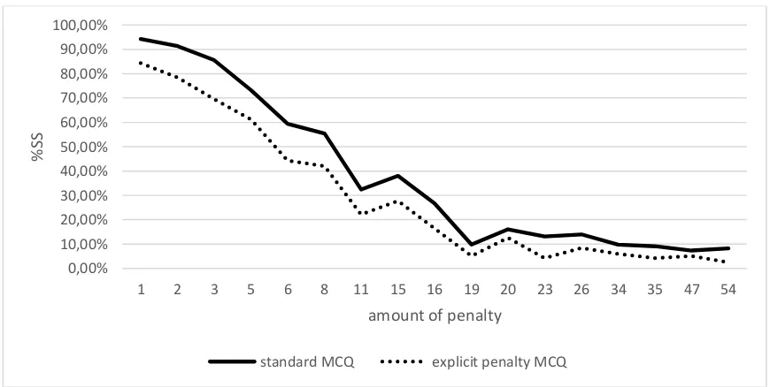
First of all, the percentage of SS preferences was increasing with delay for both standard and explicit penalty version of the monetary-choice questionnaire (Figure 2) and decreasing with the amount of money subjects have to give up in case of preference of the SS option (Figure 3). The trend is, however, more clearly defined in this second case. The difference between the percentage of SS options chosen by participants in the two questionnaires was not significant in these two analyses.
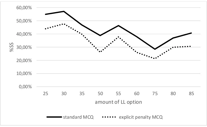
As for magnitude of the monetary reward, the percentage of the SS options for the two questionnaires were both decreasing with the amount of the LL option. This result suggests that subjects tend to decrease their level of impatience as the monetary reward increases. This is not surprising since the magnitude of a reward tends to be considered as a positive attribute of the decision problem (Lempert and Phelps, 2016). The decrease was similar, in percentage terms, in the two versions of the questionnaire, although the result of the analysis was only slightly but
significantly different (Wilcoxon test, p-value <.05). Also, subjects tested by the explicit penalty questionnaire seems to be more patient, since they are more likely to delay gratification for each LL amount (Figure 4). This is in line with the results of the discount rates analysis and, again,
descriptive data.
With the aim to further investigate this result, participants’ discount rates were also calculated for small, medium and large rewards sizes (i.e., 25-35 Euros, 50-60 Euros, and 75-85 Euros,
respectively). As a result, we found that participants discounted small magnitudes more rapidly than medium and large ones in both elicitation modes (Table 2). However, they discounted money more rapidly in the standard MCQ than in the explicit penalty mode for each of the three reward sizes (Figure 5). All these differences resulted to be statistically significant at the Wilcoxon test (Table 3). Namely, the test produced a p-value <.01 when testing the difference between discount rates obtained for small reward sizes in the two questionnaires. The p-value decreased to <.001, for medium reward sizes, and raised to <.05, for large ones. This result is consistent with previous studies using the monetary-choice questionnaire (e.g., Hendrickson, Rasmussen, and Lawyer, 2015) and also agrees with magnitude effects in intertemporal choice (Frederick, Loewenstein, and
18
By means of discount rates computed for small, medium, and large reward sizes, we also computed a geometric mean—which is less sensitive to variation of magnitude, of the participants’ discount rates. Then, we used these discount rates to compare individuals responding in the two versions of the MCQ. Statistical significance was confirmed at p-value <.01 (Wilcoxon test; Table 3).
To evaluate the robustness of the main treatment effect (i.e., change in discount rate in the two questionnaires), we performed additional analysis including the following: random blocked design, permutation test, and cluster analysis. First, personal characteristics of the sample as well as
possible session effects on the main treatment outcome, change in discount rates, were tested by using randomized block design. The results were not significant (p-values were: 0.48, for gender, 0.96, for age, and 0.85, for session). Second, the distribution-free permutation test, which is also based on randomization, confirmed a p-value of <.01 for the observed difference between the explicit penalty and the standard version of the monetary-choice questionnaire, previously tested by means of the Wilcoxon test. Third, we performed a hierarchical cluster analysis (cluster package by Maechler et al., 2016) to identify two clusters which were extracted from the discount rates
computed for each subject, independently of the type of questionnaire they were assigned to. As a result of the cluster analysis, 68% of subjects were classified in their actual questionnaire group (standard vs. explicit penalty). Moreover, the two obtained clusters were compared with the actual treatment assignment in the sample (standard vs. explicit penalty; see Experimental design section) and we found no significant difference (p-value=1), suggesting a comparability between the results of the two allocations (i.e., clusters analysis and actual distribution of the two types of
questionnaires).
We also ran a multiple logistic regression analysis, with the outcome variable being the choice of SS vs. LL options explained by personal characteristics (i.e., gender and age), location of sessions, reward size (for SS and LL options separately) and delay of options, and type of
19
4. Study 3: Strong monetary incentives
4.1. Methods
A total of 68 undergraduate students (78% females; age range, 19 to 20 years) from the Department of Law, and Political, Economic, and Social Sciences at the University of Piemonte Orientale participated in the experiment by completing an online survey within Moodle, an electronic learning environment. The survey was available on a fixed date and all participants provided informed consent.
Participants were presented a series of intertemporal choices between two different monetary options. Choices were defined by using the same methods as the pilot study (see section 2.1), except for the delay of the LL option which in this experiment was available after a delay of four weeks in every choice. As for the previous studies, two different questionnaires were prepared: standard (“Would you prefer €8 today or €11 in 1 week?”) and penal (“Would you prefer €11 in 1 week or €8 today with a penalty of €3?”).
Again, half of participants were randomly assigned to either standard version or to the explicit penalty mode. However, in this experiment, all participants were compensated for their
participation in the study. Specifically, one question was randomly chosen to be paid and the participants received their reward according to their choice in that chosen question. Please note that for each individual participant, a different random decision was extracted. For both immediate and future payments, subjects were individually met in their classroom and paid in cash at no
transaction cost. Because of this payment scheme, participants were told that they would make each choice as if it was the one they will receive as reward.
4.2. Results
Again, the percentage of subjects choosing the SS option was higher in the standard version (26%) than in the penalty mode (16%; Fisher exact test, p-value <.01).
20
21
5. Discussion and conclusions
The main aim of this paper was to investigate elicitation effects in intertemporal choice by using decision frames where, in case of preference for the SS option, the amount of money one has to give up was explicitly indicated and to make a comparison with the decision frame most commonly used in experimental literature.
The main finding was that the preference for the more delayed option was higher in the explicit penalty questionnaire than in the classical version with both real and hypothetical monetary rewards. The finding that participants were more patient in the penalty mode, rather than in the standard elicitation method, was confirmed by the computed discount rates also for each reward size.
This result is consistent with the hypothesis that individuals tend to shift their preferences in favour of more delayed options and then decrease their levels of impulsivity, when an explicit indication about the amount of money one has to give up for choosing the smaller and sooner reward is shown. Despite the arithmetic computation of the explicit penalty in each decision problem was relatively easy, and indeed the penalty varied between 1 and 54 Euros, the explicit reference to that amount triggered a shift of preference towards larger but later options, at least compared to controls, in the standard version of the questionnaire. Then, the explicit penalty appears to be used as a kind of a gentle nudge leading individuals to be more future-oriented.
A nudge is defined as “any aspect of the choice architecture that alters people’s behaviour in a predictable way without forbidding any options or significantly changing their economic incentives” (Thaler and Sunstein, 2008, p. 6). In particular, a nudge has been intended to be applied in environments characterized by complex decisions with lack of immediate feedback and difficulties in predicting or anticipating future events as in intertemporal choice. A nudge should be designed to give salience to certain behaviours or options, although the individual should be free to discard additional information, such as in this particular case (the idea that similar cues can be used in order to manipulate self-control problems is not new. In the domain of framing, see for instance Strotz (1955-56) and (Tversky and Kahneman, 1981)).
22
In our experiment, by simply displaying the arithmetic difference between the SS and the paired LL option, subjects appeared to be more future-oriented and available to wait for larger but later rewards. This result is consistent with previous empirical research that the normative principle of description invariance does not seem to hold at a behavioural level. In this specific context, individuals appeared to be more patient in the explicit penalty than in the standard version of the MCQ and there are different possible reasons for this. First of all, the explicit penalty scenario might have lead subjects to be more reflective in their consideration of the reduction in the reward amount, as a negative aspect, connected with the choice of the SS option.
But the scenario might also have placed the subject in a context of loss. In general, the delay of a reward can be considered as a loss for the decision-maker’s point of view. Nevertheless, this effect might be stronger in the explicit penalty questionnaire than in the standard decision mode. Indeed, the default option is typically represented by the SS option, in classical decision problems, but by the delayed reward, in alternative modes such as speed-up frames (Loewenstein, 1988). As noted in the introduction, in speed-up modes, subjects are first given the opportunity to choose a future reward and later provided with the possibility to select an earlier option of lesser value (Weber et al., 2007). In similar contexts, the individual has been found to perceive the delayed reward as her\his own and hence feel in a frame of loss, rather than gain, in selecting the earlier option while giving up the later one (see Lempert and Phelps, 2016). As a result, with respect to standard decision modes, waiting can be less aversive (Berns, Laibson and Loewenstein, 2007). Zhao et al. (2015) also reported similar results using opportunity costs. Loss aversion can thus be viewed as a possible way through which people increase their level of patience by choosing more often the LL option over the SS reward. Since speed-up modes are different but consistent with our description of the decision problem in the explicit penalty framing, this hypothesis seems to be plausible for explicit penalty modes as well. Moreover, loss aversion might be here further enhanced by explicitly indicating the monetary difference between the two possible options. Choice attributes are indeed more general in speed-up decision problems than explicit penalty ones, considering that the amount of reduction for the SS option is not explicitly specified (“receive a gift certificate of lesser value that day”; Weber et al., 2007).
23
gambling. For instance, empirical studies have been consistently reporting that many individuals are aware of the fact that they need to save more (e.g., Loewenstein, Prelec and Weber, 1999).
In this study, we also observed that the effect of using an explicit penalty in the decision
problem was higher for females than males. Considering that males have been typically found to be less risk-averse that females (Powell and Ansic, 1997), the fact that females seem to be more affected by this type of elicitation method may be also connected with loss aversion. However, since the study population is not well balanced between males and females, further research is needed to better understand this gender effect.
Furthermore, participants discounted small magnitudes more rapidly than medium and large ones in both elicitation modes. This is the magnitude effect, a well-established result in
experimental research on intertemporal choice for which small outcomes are discounted more than large ones (e.g., Benzion, Rapoport, and Yagil, 1989; Frederick, 1996; Thaler, 1981). The
difference between medium reward sizes in the two questionnaires was more significant than small and large sizes. The reasons underlying this difference should be also further investigated. It is worthwhile to note here that the medium sizes included in our experiment may be more easily compatible with real-life situations, at least considering a study population of students.
As for limitations, in this study we used the monetary-choice questionnaire as a tool which is typically used in experimental studies to elicit delay discounting. Nevertheless, the use of this particular questionnaire may be criticized for, at least, two main reasons. Firstly, individual discount rates would be more precisely computed by using adjusting procedures in which the amount of the reward and the delay are both adjusted according to the participant’s choices during the experiment (Myerson, Baumann and Green, 2014). Alternative methods, including the
24
and stable over time (Kirby, 2009; Myerson, Baumann and Green, 2016). These types of tasks have been also cited to be effective in determining individual differences in delay discounting (Madden and Johnson, 2010). In addition to this, the MCQ is a validated monetary discounting measure that has been widely used to assess discounting in the laboratory (Frederick, Loewenstein, and
O’Donoghue, 2002), not only in experimental economics but also in a wide range of fields in the cognitive science. In fact, the version that we used for our main experiment—that is the 27-item MCQ, is listed in the Cognitive Atlas, a collaborative project that aims to provide a knowledge base for cognitive science (Poldrack et al., 2011). As a result, we considered this tool as a valid method to investigate delay discounting, also in terms of reproducible research. Secondly, following Kirby, Petry, and Bickel (1999), discount rates were calculated using hyperbolic discounting. Despite the hyperbolic method has been found to be more descriptive of individual’s discounting than the classical utility theory model of intertemporal choice (Frederick, Loewenstein, and O’Donoghue, 2002), this formula has been also criticized in its applicability in different contexts (e.g., Rubinstein 2003). Moreover, despite future orientation and self-control are two fundamentally distinct
concepts, and indeed time orientation has specific elicitation methods (e.g., Consideration of Future Consequences Scale; see Strathman et al., 1994), we here used these two concepts as related.
Specifically, in this study, far-sighted decisions are described by both self-control, elicited by means of discount rates, and future orientation, reflected by the subject’s willingness to choose later
options. To date, the two notions are mainly linked in various areas of research (Bembenutty and Karabenick, 2004; Daly, Delaney, and Baumeister, 2015; Moffitt, 2011; Seginer, 2000; Takahashi, 2005). Accordingly, future orientation has been consistently found to have a significant role in the control of behaviour and those having problems of self-control tend to be more impulsive with their decisions and less future-oriented. For instance, the problem of self-control has been described by referring to an individual with two different selves: “a far-sighted “Planner” and a myopic “Doer.” (Thaler and Sunstein, 2008, p. 42). Also, we have previously reported that future orientation is an effort which requires self-control. Finally, as a more general note, caution should be taken when interpreting the choice of LL options as a measure, direct as well as indirect, of self-control. The choice of larger options can be indeed a behavioural tendency, which is commonly reported in non-humans, rather than a delay tolerance (see Paglieri, 2016).
25
classical discounted utility model which have been empirically observed for positive and/or negative outcomes (Faralla et al., 2011; Frederick, Loewenstein, and O’Donoghue, 2002). A field experiment testing the effect of a little piece of information, such as an explicit penalty, in real-life decision contexts (e.g., investment and saving decisions of professionals as well as general
population) would be also more interesting.
26
Appendix A. Supplementary data: Monetary-Choice Questionnaire.
Monetary-Choice Questionnaire: Standard Version
For each of the next 27 choices, please indicate which reward you would prefer: the smaller reward today, or the larger reward in the specified number of days (please circle the preferred option). 1. Would you prefer $34 today, or $35 in 186 days?
27
Monetary-Choice Questionnaire: Explicit Penalty Version
For each of the next 27 choices, please indicate which reward you would prefer: the smaller reward today, or the larger reward in the specified number of days (please circle the preferred option). 1. Would you prefer $35 in 186 days, or $34 today with a penalty of $1?
28
Appendix B. Supplementary data: instructions (adapted from Kirby, Petry, and Bickel
(1999)).
Standard Version
Please take the choices seriously: they may be for real money. After you complete the
questionnaire, a number of subjects will be randomly chosen to be paid for one of their choices in the questionnaire. The selected subjects will be paid for the same choice. Specifically, at the end of the session, one question will be randomly chosen to be paid and the selected participants will receive their reward according to their choice in that chosen question. For example, if the question number one will be randomly chosen (i.e., “Would you prefer $34 today, or $35 in 186 days?”), the extracted participants will win whatever their answered to that question of the questionnaire. If they had circled the smaller reward on that question, they will get $34 today, otherwise they will get $35 in 186 days from now. Immediate payments will be paid in cash at the end of the experimental session. For future rewards, we will join you, in the classroom, at the time your payment will be due. Because of this payment scheme, to make sure that you get the reward you prefer, you should answer every question as though it were the one you will win.
Explicit Penalty Version
29
References
Ahlbrecht, M. and M. Weber, 1997. “An empirical study on intertemporal decision making under risk.” Management Science 43(6), 813–826.
Ainslie, G.W., 1975. "Specious reward: A behavioral theory of impulsiveness and impulse control." Psychological Bulletin 82(4), 463–496.
Ainslie, G.W., 1992. Picoeconomics: The Strategic Interaction of Successive Motivational States within the Person. Cambridge, UK: Cambridge University Press.
Ainslie, G.W., 2001. Breakdown of Will. New York, NY: Cambridge University Press.
Andersen, S., G.W. Harrison, M.I. Lau, and E.E. Rutström, 2006. “Elicitation using multiple price lists”. Experimental Economics 9(4), 383–405.
Andreoni, J., M.A. Kuhn, and C. Sprenger, 2015. “Measuring time preferences: A comparison of experimental methods.” Journal of Economic Behavior & Organization 116(August), 451–464. Ariely, D. and K. Wertenbroch, 2002. “Procrastination, deadlines, and performance: Using
precommitment to regulate one's behavior." Psychological Science 13(3), 219–24.
Baumeister, R.F., 2002. “Yielding to temptation: Self-control failure, impulsive purchasing, and consumer behaviour.” Journal of Consumer Research 28(4), 670–676.
Becker, G.M., M.H. DeGroot, and J. Marschak, 1964. “Measuring utility by a single-response sequential method.” Behavioral Science 9(3), 226–232.
Bembenutty, H. and S.A. Karabenick, 2004. “Inherent association between academic delay of gratification, future time perspective, and self-regulated learning.” Educational Psychology Review 16(1), 35–57.
Benzion, U., A. Rapoport, and J. Yagil, 1989. “Discount rates inferred from decisions: An experimental study.” Management Science 35(3), 270–284.
Berns, G. S., D. Laibson, and G. Loewenstein, 2007. “Intertemporal choice-toward an integrative framework.” Trends in Cognitive Sciences 11(11), 482–488.
Breuer, W. and K.C. Soypak, 2015. “Framing effects in intertemporal choice tasks and financial implications.” RWTH Aachen University working paper.
Buchanan, J., 2008. “Opportunity cost.” In Durlauf, S.N. and E.B. Lawrence (Eds.), The New Palgrave Dictionary of Economics. New York, NY: Palgrave Macmillan.
Carmon, Z. and D. Ariely, 2000. “Focusing on the foregone: How value can appear so different to buyers and sellers.” Journal of Consumer Research 27(3), 360–370.
Champely, S., 2017. “Pwr: Basic functions for power analysis.” R package version 1.2-1. https://CRAN.R-project.org/package=pwr.
30
Evidence from capuchin monkey trading behavior.” Journal of Political Economy 114(3), 517-537.
Cohen, J., 1988. Statistical Power Analysis for the Behavioral Sciences. Hillsdale, NJ: Erlbaum. da Matta, A., F.L. Gonçalves, and L. Bizarro, 2012. “Delayed discounting: Concepts and
measures.” Psychology and Neuroscience 5(2), 135–146.
Daly. M., L. Delaney, and R.F. Baumeister, 2015. “Self-control, future orientation, smoking, and the impact.” Addictive Behaviors Reports 1, 89–96.
Duckworth, A.L. and M.E.P. Seligman, 2005. “Self-discipline outdoes IQ in predicting academic performance of adolescents.” Psychological Science 16(12), 939–944.
Eatwell, J., M. Milgate, and P. Newman (Eds.), 1998. Opportunity Cost. The new Palgrave Dictionary of Economics. London, UK: Macmillan.
Elliott, C. and D.M. Hayward, 1998. “The expanding definition of framing and its particular impact on economic experimentation.” Journal of Socio-Economics 27(2), 229–243.
Elster, J., 1979. Ulysses and the Sirens: Studies in Rationality and Irrationality. Cambridge, UK: Cambridge University Press.
Epley, N. and A. Gneezy, 2007. “The framing of financial windfalls and implications for public policy.” Journal of Socio-Economics 36(1), 36–47.
Faralla, V., F. Benuzzi, P. Nichelli, and N. Dimitri, 2011. “Gains and losses in intertemporal preferences: A behavioural study.” In Innocenti A., and A. Sirigu (Eds.), Neuroscience and the Economics of Decision Making. London, UK: Routledge.
Fassbender C., S. Houde, S. Silver-Balbus, K. Ballard, B. Kim, K.J. Rutledge, J.F. Dixon, A.M. Iosif, J.B. Schweitzer, and S.M. McClure, 2014. “The decimal effect: Behavioral and neural bases for a novel influence on intertemporal choice in healthy individuals and in ADHD.” Journal of Cognitive Neuroscience 26(11), 2455–2468.
Frederick, S., 1996. “The magnitude effect in intertemporal choice. Is it a mistake?” Carnegie Mellon University: Unpublished data. Pittsburgh.
Frederick S., G. Loewenstein, and T. O’Donoghue, 2002. “Time discounting and time preference: A critical review.” Journal of Economic Literature 40(2), 351–401.
Frederick, S., N. Novemsky, J. Wang, R. Dhar, and S. Nowlis, 2009. “Opportunity Cost Neglect.” Journal of Consumer Research 36(4), 553–561.
Frederick, S., D. Read, R. LeBouef, and D. Bartels, 2011. “Temporal references and temporal preferences: The age-delay effect in intertemporal choice.” Working paper.
31
Henderson, D.R., 2014. “Opportunity cost. The concise Encyclopedia of Economics”. Available online at: http://www.econlib.org/ library/Enc/OpportunityCost.html.
Hendrickson, K., E.B. Rasmussen, and S.R. Lawyer, 2015. “Measurement and validation of measures for impulsive food choice in obese and healthy weight humans.” Appetite 90(July), 254–263.
Herrnstein, R.J., 1981. “Self-control as response strengths.” In Bradshaw, E.S.C.M. and C.F. Lowe (Eds.), Quantification of Steady-State Operant Behaviour. North Holland, NL: Elsevier.
Houben, K. and A. Jansen, 2011, “Training inhibitory control. A recipe for resisting sweet temptations.” Appetite 56(2), 345–349.
Kahneman, D., 2012. Thinking, Fast and Slow. London, UK: Penguin Books.
Kahneman D., and A. Tversky, 1979. “Prospect theory: An analysis of decision under risk.” Econometrica 47(2), 263–291.
Kaplan, B.A., S.M. Lemley, D.D. Reed, D. Derek, and D.P. Jarmolowicz, 2014. “21- and 27-item Monetary Choice Questionnaire automated scorers.” [software]. Center for Applied
Neuroeconomics, University of Kansas.
Killeen, P.R., 2009. “An additive-utility model of delay discounting.” Psychological Review 116(3), 602–619.
Kirby, K.N., 1997. “Bidding on the future: Evidence against normative discounting of delayed rewards.” Journal of Experimental Psychology: General 126(1), 54–70.
Kirby, K.N., 2009, “One-year temporal stability of delay-discount rates.” Psychonomic Bulletin & Review 16(3), 457–46.
Kirby, K.N., and N.N. Maraković, 1996. “Delay-discounting probabilistic rewards: Rates decrease as amounts increase.” Psychonomic Bulletin & Review 3(1), 100–104.
Kirby, K.N., N.M. Petry, and W.K. Bickel, 1999. “Heroin addicts have higher discount rates for delayed rewards than non-drug-using controls.” Journal of Experimental Psychology: General 128(1), 78–87.
Kowal, B. and J.L. Falkener, 2016. “Delay discounting of hypothetical monetary rewards with decoys.” Behavioural Processes 122(January), 26–35.
Laibson, D., 1997. “Golden Eggs and Hyperbolic Discounting.” Quarterly Journal of Economics and Philosophy 112(2), 443–477.
Laibson, D., A. Repetto, and J. Tobacman, 1998. “Self-control and saving for retirement.” Brookings Papers on Economic Activity.
32
Levin, I.P., 1987. “Associative effects of information framing.” Bulletin of the Psychometric Society 25(2), 85–86.
Li, S. and X. Xie, 2006. “A new look at the ‘‘Asian disease’’ problem: A choice between the best possible outcomes or between the worst possible outcomes?” Thinking & Reasoning 12(2), 129– 143.
Li, S., Y. Sun, and Y. Wang, 2007. “50% off or buy one get one free? Frame preference as a function of consumable nature in dairy products.” Journal of Social Psychology 147(4), 413– 421.
Lichtenstein, D.R., S. Burton, and E.J. Karson, 1991. “The effect of semantic cues on consumer perceptions of reference price ads.” Journal of Consumer Research 18(3), 380–391.
Loewenstein, G., 1987, “Anticipation and the valuation of delayed consumption.” The Economic Journal 97(387), pp. 666–684.
Loewenstein, G., 1988. “Frames of mind in intertemporal choice.” Management Science 34(2), 200–214.
Loewenstein, G. and D. Prelec, 1992. “Anomalies in intertemporal choice: Evidence and an interpretation.” Quarterly Journal of Economics 107(2), 573–597.
Loewenstein, G., D. Prelec, and R. Weber, 1999. “What me worry? A psychological perspective on economic aspects of retirement.” in Henry, J. A. (Ed.), Behavioral Dimensions of Retirement Economics. Washington, DC: Brookings Institution Press.
Louie, K., M.W. Khaw, and P.W. Glimcher, 2013, “Normalization is a general neural mechanism for context-dependent decision making.” Proceedings of the National Academy of Sciences of the United States of America 110(15), 6139–6144.
Louie, K. and B. De Martino, 2014, “The neurobiology of context- dependent valuation and choice.” In Glimcher, P.W., and F. Fehr (Eds.), Neuroeconomics. Decision Making and the Brain. London, UK: Elsevier.
Madden, G.J. and P.S., Johnson, 2010, “A delay discounting primer.” In Madden, G. J. and W.K. Bickel (Eds.), Impulsivity: The Behavioral and Neurological Science of Discounting. Washington, DC: American Psychological Association.
Maechler, M., P. Rousseeuw, A. Struyf, M. Hubert, and K. Hornik, 2016. “Cluster: Cluster analysis basics and extensions.” R package version 2.0.5. https://CRAN.R-project.org/package=cluster. Magen, E., C.S. Dweck, and J.J. Gross, 2008. “The hidden-zero effect representing a single choice
33
Malkoc, S.A. and G. Zauberman, 2006. “Deferring versus expediting consumption: The effect of outcome concreteness on sensitivity to time horizon.” Journal of Marketing Research 43(4), 618–627.
Manzini, P., M. Mariotti, and L. Mittone, 2014. “A case of framing effects: The elicitation of time preferences.” School of Economics and Finance Discussion Paper No. 1405.
Marzilli Ericson, K.M., J.M. White, D. Laibson, and J. Cohen, 2015. “Money earlier or later? Simple heuristics explain intertemporal choices better than delay discounting.” NBER Working Paper No. 20948.
Mazur, J.E., 1987. “An adjustment procedure for studying delayed reinforcement.” In Commons, M.L., J.E. Mazur, J.A. Nevin, and H. Rachlin (Eds.), The Effect of Delay and Intervening Events on Reinforcement Value. Hillsday, NJ: Erlbaum.
McNeil. B.J., S.G. Pauker, H.C. Sox, and A. Tversky, 1982, “On the elicitation of preferences for alternative therapies.” New England Journal of Medicine 306(21), 1259–1262.
Mischel, W. and B. Underwood, 1974. “Instrumental ideation in delay of gratification.” Child Development 45(4), 1083–1088.
Moffitt, T.E., L. Arseneault, D. Belsky, N. Dickson, R.J. Hancox, H.L. Harrington, R. Houts, R. Poulton, B.W. Roberts, S. Ross, M.R. Sears, W. Murray Thomson, and A. Caspi, 2011, “A gradient of childhood self-control predicts health,wealth, and public safety.” Proceedings of the National Academy of Sciences of the United States of America 108(7), 2693–2698.
Myerson J., A.A. Baumann, and L. Green, 2014. “Discounting of delayed rewards: (A)theoretical interpretation of the Kirby questionnaire.” Behavioural Processes 107(September), 99–105. Myerson, J., A.A. Baumann, and L. Green, 2016, “Individual differences in delay discounting:
Differences are quantitative with gains, but qualitative with losses journal of behavioral decision making.” Journal of Behavioral Decision Making 30(2), 359–372.
O’Donoghue, T. and M. Rabin, 2001, “Choice and procrastination.” The Quarterly Journal of Economics 116(1), 121–160.
Paglieri, F., 2016. “Social choice for one: On the rationality of intertemporal decisions.” Behavioural Processes 127(June), 97–108.
Phelps, E.S. and R.A. Pollak, 1968. “On the second-best national saving and game-equilibrium growth.” Review of Economic Studies 35(2), 185–199.
Poldrack, R.A., A. Kittur, D. Kalar, E. Miller, C. Seppa, Y. Gil, D. Stott Parker, F.W. Sabb, and R.M. Bilder, 2011, “The cognitive atlas: Toward a knowledge foundation for cognitive neuroscience.” Frontiers in Neuroinformatics 5(17), 1–11.
34
Powell, M. and D. Ansic, 1997. “Gender differences in risk behaviour in financial decision-making: An experimental analysis.” Journal of Economic Psychology 18(6), 605–628.
R Core Team, 2015. “R: A language and environment for statistical computing. R Foundation for Statistical Computing, Vienna, Austria.” URL https://www.R-project.org/ (accessed on January 15th, 2016).
Rachlin, H., 1992. “Diminishing marginal value as delay discounting.” Journal of Experimental Analysis of Behavior 57(3), 407–415.
Rachlin, H. and L. Green, 1972. “Commitment, choice and self-control.” Journal of the Experimental Analysis of Behavior 17(1), 15–22.
Read, D. and P.H.M.P. Roelofsma, 2003. “Subadditive versus hyperbolic discounting: A
comparison of choice and matching.” Organizational Behavior and Human Decision Processes 91(2), 140–153.
Read, D., S. Frederick, B. Orsel, and J. Rahman, 2005. “Four score and seven years from now: The date/delay effect in temporal discounting.” Management Science 51(9), 1326–1335.
Read, D., S. Frederick, and M. Scholten, 2013. “DRIFT: An analysis of outcome framing in intertemporal choice.” Journal of Experimental Psychology: Learning, Memory, and Cognition 39(2), 573–588.
Richman, S.B., E.B. Slotter, W.L. Gardner, and C.N. DeWall, 2015. “Reaching out by changing what's within: Social exclusion increases self-concept malleability.” Journal of Experimental Social Psychology 57(March), 64–77.
Rubinstein, A., 2003. “Economics and psychology? The case of hyperbolic discounting.” International Economic Review 44(4), 1207–1216.
Ruderman, A.J., 1986. “Dietary restraint: A theoretical and empirical review.” Psychological Bulletin 99(2), 247–262.
Samuelson, P.A., 1937. “A note on measurement of utility.” Review of Economic Studies 4(2), 155– 161.
Scholten, M. and D. Read, 2006. “Discounting by intervals: A generalized model of intertemporal choice.” Management Science 52(9), 1424–1436.
Seginer, R., 2000, “Defensive pessimism and optimism correlates of adolescent future orientation: A domain-specific analysis.” Journal of Adolescent Research 15(3), 307–326.
35
Stewart, N., S. Reimers, and A.J.L. Harris, 2014. “On the origin of utility, weighting, and
discounting functions: How they get their shapes and how to change their shapes.” Management Science 61(3), 687–705.
Strathman, A., F. Gleicher, D.S., Boninger, and C.S. Edwards, 1994, “The consideration of future consequences: Weighing immediate and distant outcomes of behavior.” Journal of Personality and Social Psychology 66(4), 742–752.
Strotz, R.H., 1955-56. “Myopia and inconsistency in dynamic utility maximization.” Review of Economic Studies 23(3), 165–180.
Takahashi, T., 2005, “Loss of self-control in intertemporal choice may be attributable to logarithmic time-perception.” Medical Hypotheses 65(4), 691–693.
Thaler, R.H., 1981. “Some empirical evidence on dynamic inconsistency.” Economic Letters 8(3), 201–207.
Thaler, R.H. and C.R. Sunstein, 2008. Nudge: Improving Decisions about Health, Wealth, and Happiness. New Haven, Conn: Yale University Press.
Tversky, A. and D. Kahneman, 1981. “The framing of decisions and the psychology of choice.” Science 211(4481), 453–458.
Tversky, A. and D. Kahneman, 1986. “Rational choice and the framing of decisions.” Journal of Business 59(4), S251–S278.
Tversky, A. and D. Kahneman, 1992. “Loss aversion in riskless choice: A reference-dependent model.” Quarterly Journal of Economics 106(4), 1039–1061.
von Neumann, J. and O. Morgenstern, 1947. Theory of Games and Economic Behaviour. Princeton, NJ: Princeton University Press.
Weber, E.U., 2004. “The role of risk perception in risk management decisions: Who’s afraid of a poor old-age?” In Mitchell, O.S. and S.P. Utkus (Eds.), Pension Design and Structure: New Lessons from Behavioral Finance: Part I. Research on Decision-Making under Uncertainty.
Oxford, UK: Oxford University Press.
Weber, E.U., 2006. “Experience-based and description-based perceptions of long-term risk: Why global warming does not scare us (yet).” Climatic Change 77(1), 103–120.
Weber, E.U., E.J. Johnson, K.F. Milch, H. Chang, J.C. Brodscholl, and D.G. Goldstein, 2007. “Asymmetric discounting in intertemporal choice. A Query-Theory Account.” Psychological Science 18(6), 516–523.
36
Zauberman, G., B.K. Kim, S.A. Malkoc, and J.R. Bettman, 2009. “Time discounting and discounting time: Subjective time perception and intertemporal preferences.” Journal of Marketing Research 46(4), 543–556.
Zhang N., L.J. Ji, and Y. Li, 2017, “Cultural differences in opportunity cost consideration”. Frontiers in Psychology 8(45), 1–12.
37
Figure 1. Percentage of smaller, sooner options (%SS) chosen by gender and type of questionnaire (standard vs. explicit penalty monetary-choice questionnaire – MCQ).
0,00% 5,00% 10,00% 15,00% 20,00% 25,00% 30,00% 35,00% 40,00% 45,00% 50,00%
males females
38
Figure 2. Percentage of smaller, sooner options (%SS) chosen by participants according to the delay difference between the smaller, sooner option and the paired larger, later one by type of questionnaire (standard vs. explicit penalty monetary-choice questionnaire – MCQ).
0,00% 10,00% 20,00% 30,00% 40,00% 50,00% 60,00% 70,00% 80,00% 90,00% 100,00%
7 13 14 19 20 21 29 30 53 61 62 80 89 91 111117119136157160162179186
%S
S
delay
39
Figure 3. Percentage of smaller, sooner options (%SS) chosen by participants according to the amount of money subjects have to give up in case of preference of the smaller, sooner option by type of questionnaire (standard vs. explicit penalty monetary-choice questionnaire – MCQ).
0,00% 10,00% 20,00% 30,00% 40,00% 50,00% 60,00% 70,00% 80,00% 90,00% 100,00%
1 2 3 5 6 8 11 15 16 19 20 23 26 34 35 47 54
%S
S
amount of penalty
40
Figure 4. Percentage of smaller, sooner options (%SS) chosen by participants according to the amount of the larger, later (LL) option by type of questionnaire (standard vs. explicit penalty monetary-choice questionnaire – MCQ).
0,00% 10,00% 20,00% 30,00% 40,00% 50,00% 60,00%
25 30 35 50 55 60 75 80 85
%S
S
amount of LL option