1799
How Much Attention Do You Need?
A Granular Analysis of Neural Machine Translation Architectures
Tobias Domhan Amazon Berlin, Germany domhant@amazon.com
Abstract
With recent advances in network ar-chitectures for Neural Machine Transla-tion (NMT) recurrent models have effec-tively been replaced by either convolu-tional or self-attenconvolu-tional approaches, such as in the Transformer. While the main in-novation of the Transformer architecture is its use of self-attentional layers, there are several other aspects, such as attention with multiple heads and the use of many attention layers, that distinguish the model from previous baselines. In this work we take a fine-grained look at the different ar-chitectures for NMT. We introduce an Ar-chitecture Definition Language (ADL) al-lowing for a flexible combination of com-mon building blocks. Making use of this language, we show in experiments that one can bring recurrent and convolutional models very close to the Transformer per-formance by borrowing concepts from the Transformer architecture, but not using self-attention. Additionally, we find that self-attention is much more important for the encoder side than for the decoder side, where it can be replaced by a RNN or CNN without a loss in performance in most settings. Surprisingly, even a model without any target side self-attention per-forms well.
1 Introduction
Since the introduction of attention mecha-nisms (Bahdanau et al.,2014;Luong et al.,2015) Neural Machine Translation (NMT) (Sutskever et al., 2014) has shown some impressive results. Initially, approaches to NMT mainly relied on Recurrent Neural Networks (RNNs) (
Kalchbren-ner and Blunsom, 2013; Bahdanau et al., 2014;
Luong et al.,2015;Wu et al.,2016) such as Long Short-Term Memory (LSTM) networks ( Hochre-iter and Schmidhuber, 1997) or the Gated Recti-fied Unit (GRU) (Cho et al.,2014).
Recently, other approaches relying on con-volutional networks (Kalchbrenner et al., 2016;
Gehring et al., 2017) and self-attention (Vaswani et al., 2017) have been introduced. These ap-proaches remove the dependency between source language time steps, leading to considerable speed-ups in training time and improvements in quality. The Transformer, however, contains other differences besides self-attention, including layer normalization across the entire model, multiple source attention mechanisms, a multi-head dot at-tention mechanism, and the use of residual feed-forward layers. This raises the question of how much each of these components matters.
To answer this question we first introduce a flexible Architecture Definition Language (ADL) (§2). In this language we standardize existing components in a consistent way making it eas-ier to compare structural differences of architec-tures. Additionally, it allows us to efficiently per-form a granular analysis of architectures, where we can evaluate the impact of individual compo-nents, rather than comparing entire architectures as a whole. This ability leads us to the following observations:
• Source attention on lower encoder layers brings no additional benefit (§4.2).
• Multiple source attention layers and residual feed-forward layers are key (§4.3).
2 Flexible Neural Machine Translation Architecture Combination
In order to experiment easily with different ar-chitecture variations we define a domain specific NMT Architecture Definition Language (ADL), consisting of combinable and nestable building blocks.
2.1 Neural Machine Translation
NMT is formulated as a sequence to sequence prediction task in which a source sentence X =
x1, ..., xnis translated auto-regressively into a
tar-get sentence Y = y1, ..., ym one token at a time
as
p(yt|Y1:t−1, X;θ) = softmax(WozL+bo),
(1)
wherebois a bias vector,Woprojects a model
de-pendent hidden vectorzLof theLth decoder layer to the dimension of the target vocabularyVtrg and θdenotes the model parameters. Typically, during trainingY1:t−1 consists of the reference sequence tokens, rather then the predictions produced by the model, which is known as teacher-forcing. Train-ing is done by minimizTrain-ing the cross-entropy loss between the predicted and the reference sequence.
2.2 Architecture Definition Language
In the following we specify the ADL which can be used to define any standard NMT architecture and combinations thereof.
Layers The basic building block of the ADL is a layer l. Layers can be nested, mean-ing that a layer can consist of several sub-layers. Layers optionally take set of named ar-gumentsl(k1=v1, k2=v2, ...)with namesk1,k2, ... and values v1, v2, ... or positional arguments
l(v1, v2, ...).
Layer definitions For each layer we have a cor-responding layer definition based on the hidden states of the previous layer and any additional ar-guments. Specifically, each layer takes T hid-den states hi1, ...,hiT, which in matrix form are Hi ∈ RT×di, and produces a new set of hidden states hi1+1, ...,hiT+1 orHi+1. While each layer can have a different number of hidden units di,
in the following we assume them to stay constant across layers and refer to the model dimensionality asdmodel. We distinguish the hidden states on the
source sideU0, ...,ULs from the hidden states of
the target sideZ0, ...,ZL. These are produced by the source and target embeddings and Ls source
layers andLtarget layers.
Source attention layers play a special role in that their definition additionally makes use of any of the source hidden statesU0, ...,ULs.
Layer chaining Layers can be chained, feeding the output of one layer as the input to the next. We denote this asl1 →l2...lL. This is equivalent
to writinglL(... l2(l1(H0)))if none of the layers is a source attention layer.
In layer chains layers may also contain lay-ers that themselves take arguments. As an ex-ample l1(k=v) → l2 ... lL is equivalent
to lL(... l2(l1(H0, k=v))). Note that unlike in the layer definition hidden states are not explic-itly stated in the layer chain, but rather implicexplic-itly defined through the preceding layers.
Encoder/Decoder structure A NMT model is fully defined through two layer chains, namely one describing the encoder and another describing the decoder. The first layer hidden states on the source U0 are defined through the source embedding as
u0t =Esrcxt (2)
where xt ∈ {0,1}|Vsrc| is the one-hot
represen-tation ofxtandESxt ∈ Re×|Vsrc|an embedding matrix with embedding dimensionality e. Simi-larly,Z0 is defined through the target embedding matrixEtgt.
Given the final decoder hidden state ZL the next word predictions are done according to Equa-tion1.
Layer repetition Networks often consist of sub-structures that are repeated several times. In order to support this we define a repetition layer as
repeat(n, l) =l1l2...ln,
wherel represents a layer chain and each one of
l1, ..., lnan instantiation of that layer chain with a
separate set of weights.
2.3 Layer Definitions
Dropout A dropout (Srivastava et al., 2014) layer, denoted as dropout(ht), can be applied to
hidden states as a form of regularization.
Fixed positional embeddings Fixed positional embeddings (Vaswani et al., 2017) add informa-tion about the posiinforma-tion in the sequence to the hid-den states. With ht ∈ Rd the positional embed-ding layer is defined as
pos(ht) =dropout(
√
d·ht+pt)
pt,j = sin(t/100002j/d)
pt,2j+1= cos(t/100002j/d).
Linear We define a linear projection layer as
linear(ht, do) =Wht+b,
whereW∈Rdo×din.
Feed-forward Making use of the linear projec-tion layer a feed-forward layer with ReLU activa-tion and dropout is defined as
ff(ht, do) =dropout(max(0,linear(ht, do)))
and a version which temporarily upscales the num-ber of hidden units, as done by Vaswani et al.
(2017), can be defined as
ffl(ht) =ff(4din)linear(din)
whereht∈Rdin.
Convolution Convolutions run a small feed-forward network on a sliding window over the in-put. Formally, on the encoder side this is defined as
cnn(H, v, k) =v(W[hi−bk/2c;...;hi+bk/2c] +b)
wherekis the kernel size, andvis a non-linearity. The input is padded so that the number of hidden states does not change.
To preserve the auto-regressive property of the decoder we need to make sure to never take fu-ture decoder time steps into account, which can be achieved by adding k − 1 padding vectors h−k+1 = 0, . . . ,h−1 = 0 such that the decoder convolution is given as
cnn(H, v, k) =v(W[ht−k+1;...;ht] +b).
The non-linearity v can either be a ReLU or a Gated Linear Unit (GLU) (Dauphin et al.,2016). With the GLU we set di = 2dsuch that we can
splith = [hA;hB] ∈ R2dand compute the non-linearity as
glu([hA;hB]) =hA⊗σ(hB).
Identity We define an identity layer as
id(ht) =ht.
Concatenation To concatenate the output of p
layer chains we define
concat(ht, l1, ..., lp) = [l1(ht);...;lp(ht)].
Recurrent Neural Network An RNN layer is defined as
rnn(ht) =frnn o(ht,st−1) st=frnn h(ht,st−1)
where frnn o and frnn h could be defined
through either a GRU (Cho et al., 2014) or a LSTM (Hochreiter and Schmidhuber, 1997) cell. In addition, a bidirectional RNN layer birnn is available, which runs onernn in forward and an-other in reverse direction and concatenates both re-sults.
Attention All attention mechanisms take a set of query vectors q0, ...,qM, key vectors k0, ...,kN
and value vectors v0, ...,vN in order to produce
one context vector per query, which is a linear combination of the value vectors. We defineQ∈ RM×d, V ∈ RN×d andK ∈ RN×das the con-catenation of these vectors. What is used as the query, key and value vectors depends on attention type and is defined below.
Dot product attention The scaled dot prod-uct attention (Vaswani et al.,2017) is defined as
dot att(Q,K,V, s) = softmax
QK> √
s
V,
where the scaling factorsis implicitly set tod un-less noted otherwise. Adding a projection to the queries, keys and values we get the projected dot attention as
proj dot att(Q,K,V, dp, s) =
dot att(QWQ,KWK,VWV, s)
where dp is dimensionality of the projected
vec-tors such thatWQ∈Rdq×dp,WK ∈
Rdk×dp and WV ∈Rdv×dp.
Vaswani et al.(2017) further introduces a multi-head attention, which applies multiple attentions at a reduced dimensionality. Withhheads multi-head attention is computed as
Ci =proj dot att(Q,K,V, d/h, s).
Note that withh= 1we recover the projected dot attention.
MLP attention The MLP attention ( Bah-danau et al.,2014) computes the scores with a one-layer neural network as
mlp att(Q,K,V) = softmax (S)V,
Sij =wTo tanh(Wqqi+Wkkj).
Source attention Using the source hidden vectorsU, the source attentions are computed as
mh dot src att(H,U, h, s) =
mh dot att(H,U,U, h, s),
mlp src att(H,U) =mlp att(H,U,U),
dot src att(H,U, s) =mh dot att(H,U,U,1, s).
Self-attention Self-attention (Vaswani et al.,
2017) uses the hidden states as queries, keys and values such that
mh dot self att(H, s) =mh dot att(H,H,H, s).
Please note that on the target side one needs to make sure to preserve the auto-regressive property by only attending to hidden states at the current or past stepsh < t, which is achieved by masking the attention mechanism.
Layer normalization Layer normalization (Ba et al.,2016) uses the mean and standard deviation for normalization. It is computed as
norm(ht) =
g
σt
⊗(ht−µt) +b
µt=
1
d
d
X
i=1
ht,j σt=
v u u t 1
d
d
X
i=1
(ht,j−µj)2
wheregandbare learned scale and shift parame-ters with the same dimensionality ash.
Residual layer A residual layer adds the output of an arbitrary layer chainlto the current hidden states. We define this as
res(ht, l) =ht+l(ht).
For convenience we also define
res d(ht, l) =res(l(ht)dropout) and res nd(ht, l) =res(norml(ht)dropout).
2.4 Standard Architectures
Having defined the common building blocks we now show how standard NMT architectures can be constructed.
RNMT As RNNs have been around the longest in NMT, several smaller architecture variations exist. Similar toWu et al.(2016) in the following we use a bi-directional RNN followed by a stack of uni-directional RNNs with residual connections on the encoder side. Using the ADL annlayer en-coder can be expressed as
ULs =dropout
birnnrepeat(n−1,res d(rnn)).
For the decoder we use the architecture byLuong et al.(2015), which first runs a stacked RNN and then combines the context provided by a single at-tention mechanism with the hidden state provided by the RNN. This can be expressed by
ZL=dropoutrepeat(n,res d(rnn))
concat(id,mlp att)ff.
If input feeding (Luong et al., 2015) is used the first layer hidden states are redefined as
z0t = [zLt−1;Etgtyt].
Note that this inhibits any parallelism across de-coder time steps. This is only an issue when using models other than RNNs, as RNNs already do not allow for parallelizing over decoder time steps.
ConvS2S Gehring et al. (2017) introduced a NMT model that fully relies on convolutions, both on the encoder and on the decoder side. The en-coder is defined as
ULs =pos
repeat(n,res(cnn(glu)dropout))
and the decoder, which uses an unscaled single head dot attention is defined as
ZL=posres(dropoutcnn(glu)dropout
res(dot src att(s=1))).
Transformer The Transformer (Vaswani et al.,
2017) makes use of self-attention, instead of RNNs or Convolutional Neural Networks (CNNs), as the basic computational block. Note that we use a slightly updated residual structure as im-plemented bytensor2tensor1than proposed origi-nally. Specifically, layer normalization is applied to the input of the residual block instead of ap-plying it between blocks. The Transformer uses a combination of self-attention and feed-forward layers on the encoder and additionally source at-tention layers on the decoder side. When defining the Transformer encoder block as
tenc=res nd(mh dot self att)res nd(ffl),
and the decoder block as
tdec=res nd(mh dot self att)
res nd(mh dot src att)res nd(ffl).
the Transformer encoder is given as
ULs =pos
repeat(n,tenc)norm
and the decoder as
ZL=posrepeat(n,tdec)norm.
3 Related Work
The dot attention mechanism, now heavily used in the Transformer models, was introduced by ( Lu-ong et al.,2015) as part of an exploration of dif-ferent attention mechanisms for RNN based NMT models.
Britz et al. (2017) performed an extensive ex-ploration of hyperparameters of RNN based NMT models. The variations explored include different attention mechanisms, RNN cells types and model depth.
Similar to our work, Schrimpf et al.(2017) de-fine a language for exploring architectures. In this case the architectures are defined for RNN cells and not for the higher level model architec-ture. Using the language they perform an auto-matic search of RNN cell architectures.
For the application of image classification there have been several recent successful efforts of automatically searching for successful architec-tures (Zoph and Le,2016;Negrinho and Gordon,
2017;Liu et al.,2017).
1https://github.com/tensorflow/tensor2tensor
4 Experiments
What follows is an extensive empirical analysis of current NMT architectures and how certain sub-layers as defined through our ADL affect perfor-mance.
4.1 Setup
All experiments were run with an adapted ver-sion of SOCKEYE (Hieber et al., 2017), which can parse arbitrary model definitions that are ex-pressed in the language described in Section2.3. The code and configuration are available at
https://github.com/awslabs/sockeye/tree/acl18 al-lowing researchers to easily replicate the experi-ments and to quickly try new NMT architectures by either making use of existing building blocks in novel ways or adding new ones.
In order to get data points on corpora of differ-ent sizes we ran experimdiffer-ents on both WMT and IWSLT data sets. For WMT we ran the majority of our experiments on the most recent WMT’17 data consisting of roughly 5.9 million training sentences for English-German (EN→DE) and 4.5 million sentences for Latvian-English (LV→EN). We used newstest2016 as validation data and re-port metrics calculated on newstest2017. For the smaller IWSLT’16 English-German corpus, which consists of roughly 200 thousand training sen-tences, we used TED.tst2013 as validation data and report numbers for TED.tst2014.
For both WMT’17 and IWSLT’16 we prepro-cessed all data using the Moses2 tokenizer and
apply Byte Pair Encoding (BPE) (Sennrich et al.,
2015) with 32,000 merge operations. Unless noted otherwise we run each experiment three times with different random seeds and report the mean and standard deviation of the BLEU and ME-TEOR (Lavie and Denkowski,2009) scores across runs. Evaluation scores are based on tokenized sequences and calculated with MultEval (Clark et al.,2011).
Model WMT’14
Vaswani et al.(2017) 27.3 Our Transformerbaseimpl. 27.5
Table 1: BLEU scores on WMT’14 EN→DE.
In order to compare to previous work, we also ran an additional experiment on WMT’14 using the same data as Vaswani et al. (2017)
as provided in preprocessed form through ten-sor2tensor.3 This data set consists of WMT’16 training data, which has been tokenized and byte pair encoded with 32,000 merge operations. Eval-uation is done on tokenized and compound split newstest2014 data using multi-bleu.perl in order to get scores comparable toVaswani et al.(2017). As seen in Table1, our Transformer implementa-tion achieves a score equivalent to the originally reported numbers.
On the smaller IWSLT data we use dmodel =
512 and on WMT dmodel = 256 for all
mod-els. Models are trained with6 encoder and6 de-coder blocks, where in the Transformer model a layer refers to a full encoder or decoder block. All convolutional layers use a kernel of size 3 and a ReLU activation, unless noted otherwise. RNNs use LSTM cells. For training we use the Adam optimizer (Kingma and Ba,2014) with a learning rate of0.0002. The learning rate is decayed by a factor of 0.7, whenever the validation perplexity does not improve for 8 consecutive checkpoints, where a checkpoint is created every 4,000 updates on WMT and 1,000 updates on IWSLT. All mod-els use label smoothing (Szegedy et al.,2016) with
ls= 0.1.
4.2 What to attend to?
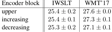
Source attention is typically based on the top en-coder block. With multiple source attention lay-ers one could hypothesize that it could be benefi-cial to allow attention encoder blocks other than the top encoder block. It might for example be beneficial for lower decoder blocks to use encoder blocks from the same level as they represent the same level of abstraction. Inversely, assuming that the translation is done in a coarse to fine manner it might help to first use the uppermost encoder block and use gradually lower level representa-tions.
Encoder block IWSLT WMT’17
upper 25.4±0.2 27.6±0.0 increasing 25.4±0.1 27.3±0.1 decreasing 25.3±0.2 27.1±0.1
Table 2: BLEU scores when varying the en-coder block used in the source attention mecha-nism of a Transformer on the EN→DE IWSLT and WMT’17 datasets.
3https://github.com/tensorflow/tensor2tensor/blob/
765d33bb/tensor2tensor/data generators/translate ende.py
The result of modifying the source attention mechanism to use different encoder blocks is shown in Table 2. The variations include using the result of the encoder Transformer block at the same level as the decoder Transformer block (increasing) and using the upper encoder Trans-former block in the first decoder block and then gradually using the lower blocks (decreasing).
We can see that attention on the upper encoder block performs best and no gains can be observed by attention on different encoder layers in the source attention mechanism.
4.3 Network Structure
The Transformer sets itself apart from both standard RNN models and convolutional model by more than just the multi-head self-attention blocks.
RNN to Transformer The differences to the RNN include the multiple source attention layers, multi-head attention, layer normalization and the residual upscaling feed-forward layers. Addition-ally, RNN models typically use single head MLP attention instead of the dot attention. This raises the question of what aspect contributes most to the performance of the Transformer.
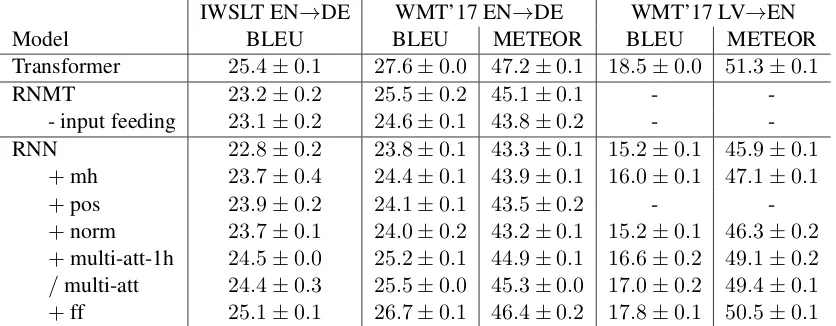
Table3shows the result of taking an RNN and step by step changing the architecture to be simi-lar to the Transformer architecture. We start with a standard RNN architecture with MLP attention similar toLuong et al.(2015) as described in Sec-tion2.4with and without input feeding denoted as RNMT.
Next, we take a model with a residual connec-tion around the encoder bi-RNN such that the en-coder is defined as
dropoutres d(birnn)repeat(5,res d(rnn)).
The decoder uses a residual single head dot atten-tion and no input feeding and is defined as
dropoutrepeat(6,res d(rnn))
res d(dot src att)res d(ffl).
[image:6.595.87.274.620.674.2]IWSLT EN→DE WMT’17 EN→DE WMT’17 LV→EN
Model BLEU BLEU METEOR BLEU METEOR
Transformer 25.4±0.1 27.6±0.0 47.2±0.1 18.5±0.0 51.3±0.1
RNMT 23.2±0.2 25.5±0.2 45.1±0.1 -
-- input feeding 23.1±0.2 24.6±0.1 43.8±0.2 - -RNN 22.8±0.2 23.8±0.1 43.3±0.1 15.2±0.1 45.9±0.1
+mh 23.7±0.4 24.4±0.1 43.9±0.1 16.0±0.1 47.1±0.1
+pos 23.9±0.2 24.1±0.1 43.5±0.2 -
-+norm 23.7±0.1 24.0±0.2 43.2±0.1 15.2±0.1 46.3±0.2 +multi-att-1h 24.5±0.0 25.2±0.1 44.9±0.1 16.6±0.2 49.1±0.2
[image:7.595.91.509.63.226.2]/multi-att 24.4±0.3 25.5±0.0 45.3±0.0 17.0±0.2 49.4±0.1 +ff 25.1±0.1 26.7±0.1 46.4±0.2 17.8±0.1 50.5±0.1
Table 3: Transforming an RNN into a Transformer style architecture. +shows the incrementally added variation./denotes an alternative variation to which the subsequent+is relative to.
upscaling feed-forward layer is added after each attention block (ff). The final architecture of the encoder after applying these variations is
posres nd(birnn)res nd(ffl)
repeat(5,res nd(rnn)res nd(ffl)norm
and of the decoder
posrepeat(6,res nd(rnn)
res nd(mh dot src att)res nd(ffl))norm.
Comparing this to the Transformer as defined in Section 2.4 we note that the model is identical to the Transformer, except that each self-attention has been replaced by an RNN or bi-RNN.
Table3 shows that not using input feeding has a negative effect on the result, which however can be compensated by the explored model variations. With just a single attention mechanism the model benefits from multiple attention heads. The gains are even larger when an attention mechanism is added to every layer. With multiple source atten-tion mechanisms the benefit of multiple heads de-creases. Layer normalization on the inputs of the residual blocks has a small negative effect in all settings and metrics. As RNNs can learn to encode positional information positional embeddings are not strictly necessary. Indeed, we can observe no gains but rather even a small drop in BLEU and METEOR for WMT’17 EN→DE when using them. Adding feed-forward layers leads to large and consistent performance boost. While the fi-nal model, which is a Transformer model where each self-attention has been replaced by an RNN, is able to make up for a large amount of the dif-ference between the baseline and the Transformer,
it is still outperformed by the Transformer. The largest gains come from multiple attention mech-anisms and residual feed-forward layers.
CNN to Transformer While the convolutional models have much more in common with the Transformer than the RNN based models, there are still some notable differences. Like the Trans-former, convolutional models have no dependency between decoder time steps during training, use multiple source attention mechanisms and use a slightly different residual structure, as seen in Sec-tion2.4. The Transformer uses a multi-head scaled dot attention while the ConvS2S model uses an un-scaled single head dot attention. Other differences include the use of layer normalization as well as residual feed-forward blocks in the Transformer.
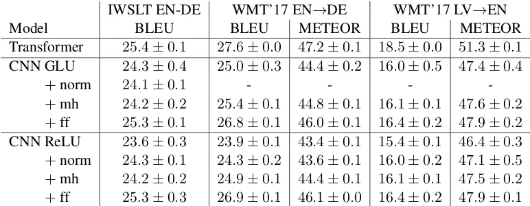
The result of making a CNN based architecture more and more similar to the Transformer can be seen in Table 4. As a baseline we use a simple residual CNN structure with a residual single head dot attention. This is denoted as CNN in Table4. On the encoder side we have
posrepeat(6,res d(cnn))
and for the decoder
posrepeat(6,res d(cnn)res d(dot src att)).
This is similar to, but slightly simpler than, the ConvS2S model described in Section2.4. In the experiments we explore both the GLU and ReLU as non-linearities for the CNN.
IWSLT EN-DE WMT’17 EN→DE WMT’17 LV→EN
Model BLEU BLEU METEOR BLEU METEOR
Transformer 25.4±0.1 27.6±0.0 47.2±0.1 18.5±0.0 51.3±0.1 CNN GLU 24.3±0.4 25.0±0.3 44.4±0.2 16.0±0.5 47.4±0.4
+norm 24.1±0.1 - - -
[image:8.595.105.491.62.212.2]-+mh 24.2±0.2 25.4±0.1 44.8±0.1 16.1±0.1 47.6±0.2 +ff 25.3±0.1 26.8±0.1 46.0±0.1 16.4±0.2 47.9±0.2 CNN ReLU 23.6±0.3 23.9±0.1 43.4±0.1 15.4±0.1 46.4±0.3 +norm 24.3±0.1 24.3±0.2 43.6±0.1 16.0±0.2 47.1±0.5 +mh 24.2±0.2 24.9±0.1 44.4±0.1 16.1±0.1 47.5±0.2 +ff 25.3±0.3 26.9±0.1 46.1±0.0 16.4±0.2 47.9±0.1
Table 4: Transforming a CNN based model into a Transformer style architecture.
identical to a Transformer where the self-attention layers have been replaced by CNNs. This means that we have the following architecture on the en-coder
posrepeat(6,res nd(cnn)res nd(ffl))norm.
Whereas for the decoder we have
posrepeat(6,res nd(cnn)
res nd(mh dot src att)res nd(ffl))norm.
While in the baseline the GLU activation works better than the ReLU activation, when layer normalization, multi-head attention attention and residual feed-forward layers are added, the perfor-mance is similar. Except for IWSLT multi-head attention gives consistent gains over single head attention. The largest gains can however be ob-served by the addition of residual feed-forward layers. The performance of the final model, which is very similar to a Transformer where each self-attention has been replaced by a CNN, matches the performance of the Transformer on IWSLT EN→DE but is still 0.7 BLEU points worse on WMT’17 EN→DE and two BLEU points on WMT’17 LV→EN.
4.4 Self-attention variations
At the core of the Transformer are self-attentional layers, which take the role previously occupied by RNNs and CNNs. Self-attention has the advantage that any two positions are directly connected and that, similar to CNNs, there are no dependencies between consecutive time steps so that the com-putation can be fully parallelized across time. One disadvantage is that relative positional information is not directly represented and one needs to rely
on the different heads to make up for this. In a CNN information is constrained to a local window which grows linearly with depth. Relative posi-tions are therefore taken into account. While an RNN keeps an internal state, which can be used in future time steps, it is unclear how well this works for very long range dependencies (Koehn and Knowles,2017;Bentivogli et al.,2016). Addi-tionally, having a dependency on the previous hid-den state inhibits any parallelization across time.
Given the different advantages and disadvan-tages we selectively replace self-attention on the encoder and decoder side in order to see where the model benefits most from self-attention.
We take the encoder and decoder block defined in Section2.4and try out different layers in place of the self-attention. Concretely, we have
tenc=res nd(xenc)res nd(ffl),
on the encoder side and
tdec=res nd(xdec)
res nd(mh dot src att)res nd(ffl).
on the decoder side. Table5 shows the result of replacing xenc andxdec with either self-attention,
a CNN with ReLU activation or an RNN. Notice that with self-attention used in bothxencandxdec
we recover the Transformer model. Additionally, we remove the residual block on the decoder side entirely (none). This results in a decoder block which only has information about the previous tar-get word yt through the word embedding that is
fed as the input to the first layer. The decoder block is reduced to
IWSLT EN→DE WMT’17 EN→DE WMT’17 LV→EN
Encoder Decoder BLEU BLEU METEOR BLEU METEOR
[image:9.595.84.516.63.213.2]self-att self-att 25.4±0.2 27.6±0.0 47.2±0.1 18.3±0.0 51.1±0.1 self-att RNN 25.1±0.1 27.4±0.1 47.0±0.1 18.4±0.2 51.1±0.1 self-att CNN 25.4±0.4 27.6±0.2 46.7±0.1 18.0±0.3 50.3±0.3 RNN self-att 25.8±0.1 27.2±0.1 46.7±0.1 17.8±0.1 50.6±0.1 CNN self-att 25.7±0.1 26.6±0.3 46.3±0.1 16.8±0.4 49.4±0.4 RNN RNN 25.1±0.1 26.7±0.1 46.4±0.2 17.8±0.1 50.5±0.1 CNN CNN 25.3±0.3 26.9±0.1 46.1±0.0 16.4±0.2 47.9±0.2 self-att combined 25.1±0.2 27.6±0.2 47.2±0.2 18.3±0.1 51.1±0.1 self-att none 23.7±0.2 25.3±0.2 43.1±0.1 15.9±0.1 45.1±0.2
Table 5: Different variations of the encoder and decoder self-attention layer.
In addition to that, we try a combination where the first and fourth block use self-attention, the second and fifth an RNN, the third and sixth a CNN ( com-bined).
Replacing the self-attention on both the encoder and the decoder side with an RNN or CNN re-sults in a degradation of performance. In most settings, such as WMT’17 EN→DE for both vari-ations and WMT’17 LV→EN for the RNN, the performance is comparable when replacing the de-coder side self-attention. For the ende-coder how-ever, except for IWSLT, we see a drop in perfor-mance of up to 1.5 BLEU points when not using self-attention. Therefore, self-attention seems to be more important on the encoder side than on the decoder side. Despite the disadvantage of having a limited context window, the CNN performs as well as self-attention on the decoder side on IWLT and WMT’17 EN→DE in terms of BLEU and only slightly worse in terms of METEOR. The combi-nation of the three mechanisms (combined) on the decoder side performs almost identical to the full Transformer model, except for IWSLT where it is slightly worse.
It is surprising how well the model works with-out any self-attention as the decoder essentially looses any information about the history of gener-ated words. Translations are entirely based on the previous word, provided through the target side word embedding, and the current position, pro-vided through the positional embedding.
5 Conclusion
We described an ADL for specifying NMT archi-tectures based on composable building blocks. In-stead of committing to a single architecture, the language allows for combining architectures on
a granular level. Using this language we ex-plored how specific aspects of the Transformer ar-chitecture can successfully be applied to RNNs and CNNs. We performed an extensive evalua-tion on IWSLT EN→DE, WMT’17 EN→DE and LV→EN, reporting both BLEU and METEOR over multiple runs in each setting.
We found that RNN based models benefit from multiple source attention mechanisms and resid-ual feed-forward blocks. CNN based models on the other hand can be improved through layer nor-malization and also feed-forward blocks. These variations bring the RNN and CNN based models close to the Transformer. Furthermore, we showed that one can successfully combine architectures. We found that self-attention is much more impor-tant on the encoder side than it is on the decoder side, where even a model without self-attention performed surprisingly well. For the data sets we evaluated on, models with self-attention on the en-coder side and either an RNN or CNN on the de-coder side performed competitively to the Trans-former model in most cases.
We make our implementation available so that it can be used for exploring novel architecture varia-tions.
References
Jimmy Lei Ba, Jamie Ryan Kiros, and Geoffrey E Hin-ton. 2016. Layer normalization. arXiv preprint arXiv:1607.06450.
Dzmitry Bahdanau, Kyunghyun Cho, and Yoshua Ben-gio. 2014. Neural machine translation by jointly learning to align and translate. arXiv preprint arXiv:1409.0473.
phrase-based machine translation quality: a case study. arXiv preprint arXiv:1608.04631.
Denny Britz, Anna Goldie, Thang Luong, and Quoc Le. 2017. Massive exploration of neural ma-chine translation architectures. arXiv preprint arXiv:1703.03906.
Kyunghyun Cho, Bart Van Merri¨enboer, Caglar Gul-cehre, Dzmitry Bahdanau, Fethi Bougares, Holger Schwenk, and Yoshua Bengio. 2014. Learning phrase representations using rnn encoder-decoder for statistical machine translation. arXiv preprint arXiv:1406.1078.
Jonathan H Clark, Chris Dyer, Alon Lavie, and Noah A Smith. 2011. Better hypothesis testing for statistical machine translation: Controlling for optimizer insta-bility. InProceedings of the 49th Annual Meeting of the Association for Computational Linguistics: Hu-man Language Technologies: short papers-Volume 2, pages 176–181. Association for Computational Linguistics.
Yann N Dauphin, Angela Fan, Michael Auli, and David Grangier. 2016. Language modeling with gated convolutional networks. arXiv preprint arXiv:1612.08083.
Jonas Gehring, Michael Auli, David Grangier, De-nis Yarats, and Yann N Dauphin. 2017. Convolu-tional sequence to sequence learning. arXiv preprint arXiv:1705.03122.
Felix Hieber, Tobias Domhan, Michael Denkowski, David Vilar, Artem Sokolov, Ann Clifton, and Matt Post. 2017. Sockeye: A Toolkit for Neural Machine Translation.ArXiv preprint arXiv:1712.05690.
Sepp Hochreiter and J¨urgen Schmidhuber. 1997. Long short-term memory. Neural computation, 9(8):1735–1780.
Nal Kalchbrenner and Phil Blunsom. 2013. Recurrent continuous translation models. In Proceedings of the 2013 Conference on Empirical Methods in Nat-ural Language Processing, pages 1700–1709.
Nal Kalchbrenner, Lasse Espeholt, Karen Simonyan, Aaron van den Oord, Alex Graves, and Koray Kavukcuoglu. 2016. Neural machine translation in linear time. arXiv preprint arXiv:1610.10099.
Diederik P Kingma and Jimmy Ba. 2014. Adam: A method for stochastic optimization. arXiv preprint arXiv:1412.6980.
Philipp Koehn and Rebecca Knowles. 2017. Six challenges for neural machine translation. arXiv preprint arXiv:1706.03872.
Alon Lavie and Michael J Denkowski. 2009. The meteor metric for automatic evaluation of machine translation. Machine translation, 23(2-3):105–115.
Hanxiao Liu, Karen Simonyan, Oriol Vinyals, Chrisan-tha Fernando, and Koray Kavukcuoglu. 2017. Hi-erarchical representations for efficient architecture search. arXiv preprint arXiv:1711.00436.
Minh-Thang Luong, Hieu Pham, and Christopher D Manning. 2015. Effective approaches to attention-based neural machine translation. arXiv preprint arXiv:1508.04025.
Renato Negrinho and Geoff Gordon. 2017. Deepar-chitect: Automatically designing and training deep architectures. arXiv preprint arXiv:1704.08792.
Martin Schrimpf, Stephen Merity, James Bradbury, and Richard Socher. 2017. A flexible approach to auto-mated rnn architecture generation. arXiv preprint arXiv:1712.07316.
Rico Sennrich, Barry Haddow, and Alexandra Birch. 2015. Neural machine translation of rare words with subword units. arXiv preprint arXiv:1508.07909.
Nitish Srivastava, Geoffrey Hinton, Alex Krizhevsky, Ilya Sutskever, and Ruslan Salakhutdinov. 2014. Dropout: A simple way to prevent neural networks from overfitting. The Journal of Machine Learning Research, 15(1):1929–1958.
Ilya Sutskever, Oriol Vinyals, and Quoc V Le. 2014. Sequence to sequence learning with neural net-works. InAdvances in neural information process-ing systems, pages 3104–3112.
Christian Szegedy, Vincent Vanhoucke, Sergey Ioffe, Jon Shlens, and Zbigniew Wojna. 2016. Rethinking the inception architecture for computer vision. In Proceedings of the IEEE Conference on Computer Vision and Pattern Recognition, pages 2818–2826.
Ashish Vaswani, Noam Shazeer, Niki Parmar, Jakob Uszkoreit, Llion Jones, Aidan N Gomez, Łukasz Kaiser, and Illia Polosukhin. 2017. Attention is all you need. InAdvances in Neural Information Pro-cessing Systems, pages 6000–6010.
Yonghui Wu, Mike Schuster, Zhifeng Chen, Quoc V Le, Mohammad Norouzi, Wolfgang Macherey, Maxim Krikun, Yuan Cao, Qin Gao, Klaus Macherey, et al. 2016. Google’s neural ma-chine translation system: Bridging the gap between human and machine translation. arXiv preprint arXiv:1609.08144.