Munich Personal RePEc Archive
Monetary policy with non-homothetic
preferences
Cavallari, Lilia
Department of Political Science, University or Rome III
February 2018
Online at
https://mpra.ub.uni-muenchen.de/85147/
Monetary policy with non-homothetic
preferences
Lilia Cavallari
University of Rome III
February 2018
Abstract
This paper studies the role of non-homothetic preferences for monetary pol-icy from both a positive and a normative perspective. It draws on a dynamic stochastic general equilibrium model characterized by preferences with a vari-able elasticity of substitution among goods and with price adjustment costs à la Rotemberg. These preferences - introduced by Cavallari and Etro (2017) in a setup with ‡exible prices - have remarkable implications for monetary policy. Three main results stand out from a comparison of models with an increasing and a constant elasticity. First, an increasing elasticity induces novel intertem-poral substitution e¤ects that amplify the propagation of monetary and tech-nology shocks. Second, it weakens the ability of a simple Taylor rule to attain a given level of macroeconomic stabilization. Third, the smallest welfare losses can be attained by stabilizing both in‡ation and output, in contrast to the pre-vailing view - based on models with a constant elasticity - that the best thing the monetary authority can do is to control in‡ation only.
Keywords: non-homothetic preferences; monetary policy; output stabiliza-tion; in‡ation stabilizastabiliza-tion; Taylor rule; new-Keynesian model; time-varying elasticity.
1
Introduction
The new Keynesian model, a dynamic stochastic general equilibrium model with monopolistic competition and sticky prices, has become the workhorse for the analysis of monetary policy. A basic framework consisting of a dynamics IS equation, a forward-looking Phillips curve, and a Taylor rule is often used for discussing optimal policy (e.g., the textbooks of Galì, 2015 and Walsh, 2010; see also Clarida, Galì and Gertler, 2000), while forecasting and the evaluation of monetary policy are mainly conducted in medium-scale models accounting for a variety of frictions and other features (for instance, Christiano, Eichenbaum and Evans, 2005; Smets and Wouters, 2007). The typical new Keynesian model - either in the basic or in the extended version - assumes homothetic prefer-ences, generally in the form of a constant elasticity of substitution among goods (CES). This assumption has several (unappealing) consequences. The demand for any two given goods depends only on their relative price and is independent of income. This stands in contrast with well-established empirical regularities in the behavior of consumers suggesting that income a¤ects the share of
expendi-ture devoted to di¤erent types of goods.1 Moreover, the marginal propensity to
consume out of disposable income seems to change systematically with the level of income and also with changes in income, being higher for individuals experi-encing income decreases and lower for individuals experiexperi-encing income increases (Attanasio and Weber, 2010). These behaviors - neglected in model based on homothetic preferences - may indeed a¤ect the way shocks are transmitted in the economy, and the main purpose of my analysis is to explore to what extent
they do so. 2
This paper puts to scrutiny the way monetary policy propagates its e¤ects and the way it should be conducted, focusing on the role of preferences. For this purpose, it considers a dynamic stochastic general equilibrium model with non-homothetic preferences belonging to the class of symmetric, directly ad-ditive preferences already used by Dixit and Stiglitz (1977), and with price adjustment costs à la Rotemberg (1982). The model draws on Cavallari and Etro (2017) for the speci…cation of preferences with a variable elasticity of sub-stitution among di¤erent varieties of goods. For expositional convenience the elasticity is assumed to be increasing in the level of consumption, yet the model easily nests the cases of a decreasing and a constant elasticity.
I start by illustrating the mechanics of monetary transmission in a basic model without capital, comparing the propagation of monetary and technology shocks under an increasing and a constant elasticity. An increasing elasticity ampli…es the real e¤ects of a shock to the Taylor rule, while dampening the e¤ects on prices. An unexpected increase in the nominal interest rate leads to
1The Engel’s law, for example, says that the proportion of expenditure devoted to food is
a decreasing function of total expenditure (Jorgenson, 1997). In general, evidence based on consumers’ behavior suggests that the demand elasticity is indeed time-varying (e.g. Attanasio and Browning, 1995).
2A key limitation of macroeconomic models based on homothetic preferences is that
a fall in output that is twice as large in the model with an increasing elasticity compared to a constant elasticity. The reason is a weak incentive to smooth out consumption in the presence of output ‡uctuations. With an increasing elastic-ity, in fact, the cost of trading-o¤ maintaining a high level of consumption today (when income declines most), for a slightly declining consumption path in the future is relatively high and the consumer will rather prefer to reduce consump-tion on the impact of the shock (when the elasticity is low), while maintaining a consumption path as high as possible in the future (when the elasticity is high). On the other side, the shock implies a smaller fall in in‡ation, for …rms take advantage of a low elasticity in the early part of the transition to revise their desired markups upwards. For similar motives, an increasing elasticity ampli-…es both the output and the price e¤ects of shocks, like technology shocks, that move prices and quantities in opposite directions.
I then extend the model to account for the role of capital in a setup with an increasing elasticity. The introduction of capital has the usual e¤ect of maintain-ing consumption as smooth as possible, and let output ‡uctuations be absorbed almost entirely by investments. A time-varying elasticity is key for the timing and magnitude of the propagation of shocks: both monetary and technology shocks have larger real e¤ects when the elasticity is increasing, for reasons sim-ilar to those considered in the model without capital. In addition, their e¤ects are much more persistent, since changes in the demand elasticity induce in-tertemporal substitution of expenditure decisions that favour the accumulation of capital.
2
The basic model without capital
The basic model has the purpose of illustrating the mechanics of monetary transmission in a framework with non-homothetic preferences. To set notation, the exposition is based on Cavallari and Etro (2017). The economy is populated by a unitary mass of agents, who are consumers, workers and entrepreneurs. The
labor inputLtis entirely employed by a perfectly competitive sector producing
an intermediate good with a linear technology. The intermediate good can be used to produce a variety of downstream …nal goods of unit mass, each of them produced with an identical linear technology. The utility function is:
U =E "1
X
t=1
t 1 logU
t
L1+t '
1 +'
!#
(1)
where E[ ] is the expectations operator, 2 (0;1) is the discount factor, Lt
is labor supply, ' 0 is the inverse of the Frisch elasticity, 0 is a scale
parameter for the disutility of labor and Ut is a utility functional of the
con-sumption of …nal goods, which is assumed symmetric on the mass of goods. This intratemporal utility is directly additive:
Ut= 1 R 0
u(Cjt)dj (2)
where the subutilityu(C)satis…esu0(C)>0andu00(C)<0. Following Cavallari
and Etro (2017), I depart from the traditional speci…cation used in macroeco-nomics, which is based on “log-CES” homothetic preferences, and consider a
polynomial speci…cation combining a linear and a power function3:
u(C) = C+
1C
1
with >1 (3)
The elasticity of substitution between goods is#(C) = (1+ C1)and is
increas-ing (decreasincreas-ing) in consumption if >(<) 0. Of course this subutility reduces
to the CES case for = 0:Although both cases are in principle possible, herein
I focus on an increasing elasticity of substitution, IES for short.
The starting point of the analysis is the system of equations describing the general equilibrium, with the new-Keynesian Phillips curve (NKPC) already in its linearized form around the zero steady-state in‡ation rate. The derivation of the system from …rst principles can be found in Cavallari and Etro (2017), while the derivation of the Phillips curve is in the Appendix. The general equilibrium is given by:
L't = ( C
1
t + 1) 1
( Ct1 + 1)Ct
Wt (4)
3These preferences belong to the more general class of symmetric implicit CES utility, see
( Ct1 + 1) 1
( Ct1 + 1)Ct
= E[ 1 +it
1 + t+1
( Ct1+1+ 1) 1
( Ct1+1+ 1)Ct+1
] (5)
it=i+ t+ t (6)
t= E[ t+1] mt mdt (7)
Yt=Ct (8)
where Ct is aggregate consumption, Wt is the real wage, it is a one-period
nominal interest rate, t is the in‡ation rate between periods t-1 and t, t
is a mean-zero monetary policy shock, mt is the (linearized) markup, and md
t
is the (linearized) desired markup. Equation (4) is the consumer’s …rst order condition for labor, equation (5) is the Euler equation for a one-period nominal bond, equation (6) is the Taylor rule, equation (7) is the NKPC, where
#(C) 1
>0, and 0 is the Rotemberg cost parameter, and equation (8) is the resource constraint. Variables without a time subscript denote steady-state values.
In a setup with a time-varying elasticity, also markups are time-varying. In
particular, the desired markup over marginal costs de…ned as Mdt = #(Ct)
#(Ct) 1
is increasing (decreasing) with the level of consumption when < (>) 0: In
linearized form it is given by:
md
t=
C1
#(C)(1 #(C))ct
where lowercase letters denote percentage deviations from steady state, e.g. ct
(Ct C)=C:The desired markup is distinct from the actual markupMt, which
is inversely related to real marginal costs, in linearized form mt= wt: Price
setting frictions imply a wedge between actual and desired markups, precisely:
Mt= M
d t
1 2 2
t 1 #(C)(1 + t) t
This wedge in turn a¤ects in‡ation through the Phillips curve (7): in‡ation will be positive when …rms expect actual markups to be below their desired level, for in that case …rms are willing to pay the adjustment cost and set higher prices to realign their markup to the desired level.
The system (4)-(8) can be conveniently reduced to get two equations in two
endogenous variables,yt and t: In linearized form around a steady state with
C=Y = 1, it reads:
yt= Eyt+1+ t E t+1+ t (9)
where 1 + ( +1) 11 ( +1
1)
<0and 1 +'+ ( +
1)
>
0:The slope of the Phillips curve is an increasing function of the parameter :
given all other parameters, an increasing elasticity, namely a positive ;implies
a smaller trade-o¤ between in‡ation and output.
The exogenous factor, and unique state variable, is the monetary policy
shock t. The system (9)-(10) can be solved by the method of undetermined
coe¢cients. Assume that the equilibrium decision rule and pricing function are linear functions of the state variable:
yt=a t and t=b t
whereaandbare unknown. Suppose that the monetary policy shock follows a
stationary AR(1) process:
t+1= t+&t+1 (11)
where&t+1 is an innovation. Substituting the guesses into the system (9)-(10),
and evaluating the expectations using the AR(1) process gives unique equilib-rium coe¢cients:
a = (1 )
( 1) (1 ) + ( ) <0 (12)
b =
( 1) (1 ) + ( ) <0
A, say, positive shock to the nominal rate (an increase in t) leads to a decline
in both in‡ation and output. The former is a consequence of the Taylor rule: on the impact of the shock, in‡ation must decline to absorb the spike in the nominal interest rate. Over time, the pressure on the nominal rate will gradually die o¤ and the in‡ation rate will return to the steady-state level. The dynamics of output is governed by the Phillips curve (7): output declines whenever in‡ation is below the expected rate and markups are above their desired level.
An increasing elasticity of substitution (i.e. a positive ) a¤ects the
equilib-rium coe¢cients (12) through the terms and :The former re‡ects
intertem-poral substitution of expenditure decisions and is governed by the marginal
utility of income. A high implies a weak incentive to smooth out consumption
over time (small in absolute value). Consider, for instance, a decline in output
(income). With a constant elasticity, the consumer will trade-o¤ maintaining a relatively high level of consumption today (when income declines most), for a slightly declining consumption path in the immediate future. With an increas-ing elasticity, however, the cost of doincreas-ing so is relatively high and the consumer will have an incentive to reduce consumption on the impact of the shock (when the elasticity is low), while maintaining a consumption path as high as possible in the future (when the elasticity is high). Clearly, this works in the direction of
2 4 6 8 10 12 14 16 18 20 -0.03
-0.02 -0.01
0 output
2 4 6 8 10 12 14 16 18 20
-0.015 -0.01 -0.005 0
[image:8.612.182.562.128.263.2]inflation
Figure 1: IRF to a one percent rise in the nominal interest rate in the IES model (solid line) and in the CES model (dashed line).
The second term re‡ects optimal pricing decisions. An increasing elasticity im-plies a weak incentive for …rms to adjust prices in response to shocks which move prices and quantities in the same direction (the opposite is true for supply shocks). An unexpected, say, fall in aggregate demand, by reducing the demand elasticity today compared to tomorrow, induces …rms to set temporarily high markups. This in turn generates a lower pressure on reducing prices when the
shock hits (low b in absolute value). An increasing elasticity therefore implies
more quantity movements and less price movements compared to a constant elasticity in response to demand shocks.
I now proceed numerically to illustrate the quantitative implications of an increasing elasticity, comparing the macroeconomic dynamics in the CES model ( = 0) and in the IES model ( >0). To facilitate the comparison the prefer-ence parameters re‡ect a steady-state markup of 25 percent in both models, in line with the average markup found in US data. In the CES model, this implies
= 5: In the IES model, where the markup depends on both and (recall
that steady-state consumption is equal to one), = 1:8 and = 1:79. 4 The
remaining parameters are fairly standard: the discount factor is = 0:99, the
Frisch elasticity is'= 1;the persistence of the monetary shock is = 0:8;the
coe¢cient of in‡ation in the Taylor rule is = 1:5, and the Rotemberg cost is
set to mimic an average duration of price rigidity of 3.3 quarters as in US data.5
In Figure 1 a one percent positive shock to the Taylor rule reduces output on
4These values are the posterior mean of the distribution of the parameters of a DSGE
model with IES preferences estimated by Cavallari and Etro (2017).
5For the calibration of I use the standard mapping between Rotemberg and Calvo pricing:
(1 ) (1 )
=#(C) 1
impact by roughly one percent in the CES model and by more than 2 percent in the IES model. The e¤ect on in‡ation is, on the contrary, almost twice as high in the CES (1.3 percent) compared to the IES model (less than 0.7 percent). As already mentioned, time-varying elasticity (and markups) amplify the real e¤ects of price stickiness: a declining demand elasticity in the early part of the transition, in fact, induces …rms to temporarily increase their markups while consumers have an incentive to postpone their expenditures in the future. These behaviors result in a small e¤ect on in‡ation and a large e¤ect on output. Opposite conclusions would hold with a decreasing elasticity.
It is illustrative to consider two extreme cases of price rigidity. First, assume
that prices are perfectly ‡exible ( = 0) ! 1). The equilibrium coe¢cients
becomea!0and b! ( 1 ) :output is independent of the monetary shock
while monetary policy is in complete control of in‡ation.6 Under ‡exible prices,
the system (9)-(10) becomes recursive and the classical neutrality holds. A
time-varying elasticity has no impact on the equilibrium of the model in this
case. On the opposite extreme, when prices are perfectly …xed ( =1 ) !
0), in‡ation is independent of the monetary shock while monetary policy is in
complete control of output (the equilibrium coe¢cients become a ! (11)
andb!0):An increasing elasticity leads to a larger output e¤ect (low ):
2.1
The business cycle
For comparison with business cycle models, it is instructive to consider the
implications of an increasing elasticity for the propagation of technology shocks.7
Assume that labor productivityAtfollows a stationary AR(1) process:
At=%At 1+at+1 (13)
whereat+1 is an innovation. A rise in labor productivity reduces the real
mar-ginal cost and increases the markup, i.e. mt= wt+At, thereby reducing
in‡ation for a given level of output. The Phillips curve modi…es as follows:
t= E[ t+1] yt 'At
Figure (2) compares the impulse response functions to a 1 percent rise in labor productivity under an increasing and a constant elasticity. These simulations are obtained for the same parameterization as before, while the new parameter
measuring the persistence of the productivity shock is set at%= 0:95:
6Equilibrium in‡ation can also be derived as the forward solution of (9) fory
t= 0;yielding: t= 1
1
X
j=1 1 j
Et t+j= 1
t
Under ‡exible prices, the Fisherian principle holds and in‡ation is only determined by the expected path of the monetary shock.
7Cavallari and Etro (2017) study the macroeconomic implications of an increasing elasticity
2 4 6 8 10 12 14 16 18 20 0
0.002 0.004 0.006 0.008
0.01 output
2 4 6 8 10 12 14 16 18 20 10-3
-3 -2.5 -2 -1.5 -1 -0.5
0 inflation
2 4 6 8 10 12 14 16 18 20 10-3
-5 -4 -3 -2 -1
0 nominal interest rate
2 4 6 8 10 12 14 16 18 20 10-3
-2 -1.5 -1 -0.5
[image:10.612.178.532.129.302.2]0 ex ante real interest rate
Figure 2: IRF to a one percent rise in labor productivity in the IES model (solid line) and in the CES model (dashed line).
In contrast to what happens after a monetary shock, where an increasing elasticity ampli…es the output e¤ects while reducing the impact on in‡ation, now the responses of both output and in‡ation are larger in the IES model than in the CES model. With a constant elasticity, the shock drives markups above the (constant) desired level, inducing …rms to pay the adjustment cost and reduce prices in the attempt to realign the markup to the desired level. This incentive is particularly strong when the elasticity is increasing, for the desired markup will decline on the impact of the shock and will stay below the steady-state level for
a while, widening the gap between actual and desired markups.8 Notice that the
Taylor rule contributes to amplifying the propagation of the shock: the decline in in‡ation leads to a drop in both the nominal and the ex-ante real interest
rate,rt it E[ t+1];accommodating the expansionary impulse of the shock.
For the reasons already mentioned, this e¤ect is larger when the elasticity is increasing.
3
The model with capital
When capitalKtis introduced into the model, the general equilibrium modi…es
as follows:
8The decline inmd
t more than compensates the fact that actual markups react less in the
IES model compared to the CES model. Mechanically, the impact onmtis proportional to ,
L't = ( C
1
t + 1) 1
( Ct1 + 1)Ct
Wt (14)
( Ct1 + 1) 1
( Ct1 + 1)Ct
= E[ (1 +Rt+1 ) ( C
1
t+1+ 1) 1
( Ct1+1+ 1)Ct+1
] (15)
( Ct1 + 1) 1
( Ct1 + 1)Ct
= E[ 1 +it
1 + t+1
( Ct1+1+ 1) 1
( Ct1+1+ 1)Ct+1
] (16)
Yt=KtL1t with 2(0;1) (17)
Wt
Rt
=1 Kt
Lt
(18)
Mt= Rt Wt
1
1
(19)
it=i+ t+ t (20)
t= E[ t+1] mt mdt (21)
Yt=Ct+Kt+1+ (1 )Kt (22)
where 2 (0;1) is the depreciation rate and Rt is the rental rate of capital.
Two new equations add the two new endogenousKt andRt: (15) is the Euler
equation for capital and (18) is the condition for the optimal mix of capital and labor in the production function (17), which equates the marginal rate of substitution between labor and capital to the relative factor prices. The accu-mulation of capital has important e¤ects for the propagation of shocks. First, it provides a natural means for the economy to smooth out consumption in the presence of ‡uctuations in income: in the resource constraint (22) investments allow consumption to move away from output. Second, it a¤ects the Phillips curve via its impact on markups.
The system (14)-(22) can be reduced to four equations for the endogenousct,
yt; kt, and t, which when linearized around a steady state withL= 1become:
ct= Ect+1+ t E t+1+ t (23)
ct= Ect+1+RE( ct+1+
'+ 1 1 yt+1
'+ 1
1 kt+1) (24)
t= E[ t+1] ct
'+
1 yt+
('+ 1)
yt=
C Yct+
K
Y (kt (1 )kt 1) (26)
where = 1 + C1
" 1
( Ct1+1) 1
1
( Ct1+ 1)
#
<0, and =#(C)(1C1#(C)) <
0. Here, (23) is the same as in the basic model without capital (recall that
ct = yt in the basic model), (25) and (26) are also the same once we posit
= 0 and kt = 0. The key di¤erence is the Euler equation for capital (24),
where the presence of capital breaks the close connection between output and
consumption, i.e. ct6=yt;and allows to smooth out consumption in the presence
of output ‡uctuations as in a standard real business cycle model. Here, changes
in consumption over time, ct Ect+1, re‡ect changes in the ex-ante real
interest rate (the term in brackets): a high rate implies an incentive to trade-o¤ a reduction in consumption today for a growing path of consumption in the
immediate future (recall that is negative). Notice that movements in the real
rate transmit to consumption in proportion to the steady-state value of the real
rate, which is typically small in standard calibrations (R= 1 (1 ) = 0:0351
in the baseline parameterization).
To gauge the macroeconomic implications of an increasing elasticity, I pro-ceed numerically using the same parameterization as in the model without capital, except for the preference parameters in the IES model, as now the
steady-state value of consumption is equal to 1.98.9 Figure 3 shows the impulse
responses in the IES and the CES models in the wake of a positive shock to the Taylor rule.
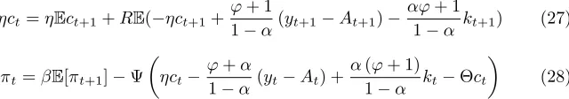
The shock reduces prices and quantities as in the model without capital. The decline in output, however, is absorbed almost entirely by investments, especially on impact when the response of consumption is close to zero. As already mentioned, the presence of capital allows consumers to maintain con-sumption as smooth as possible and this is true independently of ‡uctuations in the demand elasticity. An increasing elasticity (and countercyclical markups) are key for the timing and magnitude of the propagation: the monetary shock has larger and more persistent real e¤ects when the elasticity is increasing. The reasons are similar to those considered in the model without capital: a relatively low elasticity on the impact of the shock provides an incentive to reduce current expenditures in exchange for an increasing expenditure path in the future. In addition, the presence of capital shifts the burden of adjustment on investments (rather than consumption), making the whole transition much more persistent (capital is a state variable). With an increasing elasticity, investments take almost twice as long to converge to the steady state compared to the case of a constant elasticity. In contrast to the model without capital, an increasing elasticity has only minor consequences for in‡ation. The reason is a strong con-sumption smoothing, which dampens the variability of the desired markup and therefore aligns the dynamics of prices to the case of a constant elasticity.
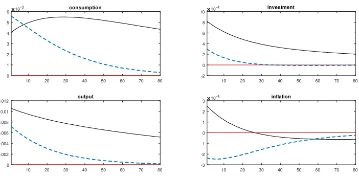
An increasing elasticity has a major impact on the propagation of technology shocks (see Figure 4). Assume that total factor productivity is an AR(1) process
10 20 30 40 50 60 70 80 10-3
-4 -3 -2 -1 0 1
2 consumption
10 20 30 40 50 60 70 80 10-4
-15 -10 -5 0
5 investment
10 20 30 40 50 60 70 80 -0.015
-0.01 -0.005
0 output
10 20 30 40 50 60 70 80 10-3
-20 -15 -10 -5 0
[image:13.612.179.530.127.302.2]5 inflation
Figure 3: IRF to a one percent rise in the nominal interest rate in the IES model (solid line) and in the CES model (dashed line).
given by (13). The shock a¤ects the dynamics of factor prices through its impact on the marginal products of labor and capital, modifying the Euler equation for capital and the Phillips curve as follows:
ct= Ect+1+RE( ct+1+'+ 1
1 (yt+1 At+1)
'+ 1
1 kt+1) (27)
t= E[ t+1] ct
'+
1 (yt At) +
('+ 1)
1 kt ct (28)
In (27), a positive shock tends to reduce the ex-ante real rate given all other conditions, thereby boosting current consumption. On the impact of the shock,
when the stock of capital is given, the e¤ect is larger the higher in absolute
value (and this explains a high initial response when the elasticity is constant in Figure 4). Over time, it depends positively on the accumulation of capital, which works in the direction of reducing the real rate, and is therefore larger with an increasing elasticity. The shock a¤ects the Phillips curve through the dynamics of markups. With a constant elasticity, falling marginal costs drive markups above the constant desired level (the …rst three addends in (28)), inducing …rms to reduce prices and realign their markups to the desired level. Consequently, in‡ation declines. With an increasing elasticity, the sign of the response is a priori ambiguous as the fall in marginal costs is accompanied by a drop in the desired markups (the fourth addend in (28)).
[image:13.612.156.476.432.488.2]10 20 30 40 50 60 70 80 10-3
0 1 2 3 4 5
6 consumption
10 20 30 40 50 60 70 80 10-4
-2 0 2 4 6 8
10 investment
10 20 30 40 50 60 70 80 0
0.002 0.004 0.006 0.008 0.01
0.012 output
10 20 30 40 50 60 70 80 10-4
-3 -2 -1 0 1 2
[image:14.612.179.530.128.302.2]3 inflation
Figure 4: IRF to a one percent rise in total factor productivity in the IES model (solid line) and in the CES model (dashed line).
without capital. As already noted, the presence of capital shifts the burden of adjustment from consumption to investments, increasing macroeconomic per-sistence. In contrast to the model without capital, in‡ation rises on the impact of the shock when elasticity is increasing and remains positive for quite a long time before converging to the steady state from below. The reason is a decline in the desired markup in the early part of the transition when the elasticity stays above the steady-state level.
4
Monetary policy design
the performance of the Taylor rule in the wake of a monetary policy shock. The e¢cient allocation can be determined by solving the problem of a benev-olent social planner seeking to maximize the representative consumer’s welfare, given technology and preferences, subject to the resource constraints. As is well-known the e¢cient allocation coincides with the equilibrium allocation un-der ‡exible prices, also called the natural allocation, once an optimal subsidy is assumed that exactly o¤sets the market power distortion. In these conditions, a policy that stabilizes …rms’ marginal costs at a level consistent with their desired markup, at unchanged prices can attain the e¢cient allocation.
In the model with capital the e¢cient allocation is given by:
L't = ( C
1
t + 1)
( Ct1 + 1)Ct
Wt (29)
( Ct1 + 1) ( Ct1 + 1)Ct
= E[ (1 +Rt+1 ) ( C
1
t+1+ 1)
( Ct1+1+ 1)Ct+1
] (30)
( Ct1 + 1) ( Ct1 + 1)Ct
= E[ 1 +it
1 + t+1
( Ct1+1+ 1)
( Ct1+1+ 1)Ct+1
] (31)
Yt=AtKtL
1
t with 2(0;1)
Wt= (1 )At
Kt
Lt
(32)
Rt= At
Kt
Lt
1
(33)
it=i+ t+ t (34)
Yt=Ct+Kt+1+ (1 )Kt (35)
In linearized form around the steady state withL= 1, the system (29)-(35)
reads:
ect= Eect+1+ t E t+1+ t (36)
e
ct= Eect+1+RE(yet+1 kt+1) (37)
e
ct=
'+
1 (yet At)
('+ 1)
1 ekt (38)
e
yt=
C Yect+
K
where a tilde denotes a variable in the e¢cient allocation. The natural equi-librium is recursive, (37), (38) and (39) determineect,yet, andektwhile in‡ation
is pinned down from (36). Therefore, monetary policy is neutral and monetary
shocks a¤ect only in‡ation. The optimal policy requires that t= 0andyt=eyt
in each period.
The utility losses experienced by the representative consumer as a conse-quence of deviations from the e¢cient allocation are expressed in terms of the equivalent permanent consumption decline, measured as a fraction of steady-state consumption. The second-order approximation to these losses yields the (average) welfare loss function, given by a linear combination of the variances of the output gap and in‡ation:
Lt= 1
2 1 +
'+
1 var(yt yet) +
#(C)
var( t)
Notice that the weight of output gap ‡uctuations in the loss is increasing in
the “curvature parameters”'and , because large values of these parameters
amplify the e¤ect of deviations from the e¢cient allocation. The weight of in‡ation ‡uctuations is instead increasing in the steady-state elasticity of sub-stitution among goods, for a high elasticity ampli…es the consumption e¤ect of any given price dispersion. The weight of in‡ation is also increasing with the
degree of price stickiness (which is inversely related with ), since the latter
ampli…es the price dispersion associated with any deviation from the optimal in‡ation rate.
Consider the following interest rate rule
it=i+ t+ yt
where >0.
Table 1 reports the standard deviation of output, the output gap and in-‡ation (all expressed in percentage terms) for di¤erent con…gurations of the
parameters and , as well as the welfare loss implied by the deviations from
the e¢cient allocation. The top panel refers to the IES model while the bot-tom panel reports results for the CES model. In both cases, the analysis is conducted conditional on the technology shock, where the standard deviation of the innovation in the technology process is set to one percent. In each panel, the …rst column reports results for the baseline calibration of the Taylor rule, which assigns a zero weight to output stabilization. The second column refers to the original calibration proposed by Taylor (1993), the third and fourth columns are based on rules involving, respectively, either a strong motive for output
stabilization ( = 1) or a strong anti-in‡ationary stance ( = 5), and the …fth
column combines both anti-in‡ationary and output stabilization motives. The remaining parameters are calibrated at the values reported above for the model with capital.
IES Model
= 1:5 = 1:5 = 1:5 = 5 = 5
= 0 = 0:125 = 1 = 0 = 0:125
(y) 9.64 8.68 4.17 9.57 9.44
( ) 0.01 2.16 8.04 0.01 0.29
(y ye) 7.21 6.10 0.99 7.14 7.0
L 0.76 1.42 12.3 0.73 0.71
CES Model
= 1:5 = 1:5 = 1:5 = 5 = 5
= 0 = 0:125 = 1 = 0 = 0:125
(y) 2.82 2.61 1.67 2.84 2.82
( ) 0.16 0.77 3.24 0.02 0.11
(y ye) 0.98 1.20 2.14 0.96 0.99
L 0.02 0.13 2.05 0.01 0.02
The table reports the standard deviation of a variable x (x)in percentage terms.
Several results stand out. For given parameters and , the Taylor rule
appears to be less e¤ective in stabilizing the economy in the IES model com-pared to the CES model: an increasing elasticity, by amplifying business cycle ‡uctuations, requires a far more aggressive policy to obtain a given level of sta-bilization. Second, the usual policy trade-o¤ between output stabilization on the one hand and stabilization of in‡ation and the output gap on the other hand emerges when elasticity is constant (CES model): increasing leads to a reduc-tion in the volatility of output and to an increase in the volatility of in‡areduc-tion and the output gap, and hence to larger welfare losses. The best-performing
rule is characterized by a strong anti-in‡ationary stance ( = 5) and no motive
for output stabilization ( = 0). This rule is very close to the optimal policy,
im-plying a permanent reduction in consumption relative to the e¢cient allocation as low as 0.01 percent.
Remarkably, this trade-o¤ disappears with an increasing elasticity, and stabi-lizing output is equivalent to stabistabi-lizing the output gap. The monetary authority can in fact weaken the ampli…cation brought about by an increasing elasticity by reducing the ‡uctuations of output and its components. In so doing, she will help align markups to their desired level and hence stabilize natural out-put. A su¢ciently large gain in terms of output stabilization may more than
compensate the loss in terms of in‡ation, so that an increase in might turn
welfare-improving (with a time-varying elasticity the welfare function becomes a non-monotonic function of ). In the baseline calibration, this happens, for instance, when a moderate motive for output stabilization is combined with a strong anti-in‡ationary stance. Among the rules considered in Table 1, the best
approximation to the optimal policy is a rule with = 5and = 0:125;leading
can be attained when the monetary authority responds to both in‡ation and
output. 10
I now turn to evaluate the performance of the simple Taylor rule in the wake of a shock that moves prices and quantities in the same direction (a demand shock). The analysis is conducted conditional on the shock to the Taylor rule (11), where the standard deviation of the innovation is set to one percent. Table 2 reports the results.
T able2Evaluation of Taylor rule (nominal shock) IES Model
= 1:5 = 1:5 = 1:5 = 5
= 0 = 0:125 = 1 = 0
(y) 5.15 4.28 1.63 0.79
( ) 2.77 2.27 1.54 0.43
(y ye) 5.15 4.28 1.63 0.79
L 1. 83 1. 24 0.49 0.04
CES Model
= 1:5 = 1:5 = 1:5 = 5
= 0 = 0:125 = 1 = 0
(y) 2.83 2.40 1.13 0.43
( ) 2.70 2.24 0.96 0.43
(y ye) 2.83 2.40 1.13 0.43
L 1. 50 1.03 0.19 0.04
When nominal shocks are the source of ‡uctuations, the policy trade-o¤ disappears also in the CES model as natural output remains unchanged, and output stabilization is equivalent to output gap stabilization. Increases in either or are e¤ective in reducing the volatility of, respectively, in‡ation and output, and reducing welfare losses in both models. As before and essentially for the same reasons, the degree of stabilization attained with a given rule is much smaller with an increasing than with a constant elasticity.
5
Concluding remarks
This paper has evaluated the role of non-homothetic preferences for monetary policy from both a positive and a normative perspective, drawing on a dynamic stochastic general equilibrium model characterized by preferences with a vari-able elasticity of substitution among goods. These preferences - introduced by Cavallari and Etro (2017) in a setup with ‡exible prices - have remarkable impli-cations for monetary policy. Three main results stand out. First, an increasing elasticity ampli…es the propagation of monetary and technology shocks, for it induces intertemporal substitution e¤ects that reduce consumption smoothing and a¤ect …rms’ desired markups. Second, an increasing elasticity weakens the
1 0Experimentations with low values for and ;which work in the direction of increasing
ability of a simple Taylor rule to attain a given level of macroeconomic stabi-lization. Third, the monetary authority can attain the smallest welfare losses by stabilizing both in‡ation and output, in contrast to the conventional wisdom - based on models with a constant elasticity - suggesting that the best thing the monetary authority can do is to control in‡ation only.
The speci…cation of preferences proposed in the paper lends itself to sev-eral applications. The model can be easily extended to account for features - like endogenous …rm entry and bank credit - that a¤ect monetary transmis-sion, opening the way to novel interactions between market demand and the dynamics of …rms and the credit channel. Moreover, the monetary setting can be amended to incorporate the presence of a zero lower bound and allow a role for unconventional policies.
Second, the intertemporal e¤ects arising in my setup with a time-varying elasticity can play a role also for macroeconomic interdependence and the inter-national monetary transmission, shedding new light on traditional policy issues, as the choice of the exchange rate regime and the gains to international monetary policy coordination. Finally, the introduction of non-homothetic preferences al-lows to address important questions about the distribution of income and the distributive consequences of monetary policy.
References
[1] Attanasio Orazio and Martin Browning, 1995, Consumption over the
Life-cycle and over the Business Life-cycle", American Economic Review vol. 85, 5,
1118-37
[2] Attanasio Orazio and Guglielmo Weber, 2010, Consumption and Saving: Models of Intertemporal Allocation and their Implications for Public Policy,
Journal of Economic Literature 48, 693-751
[3] Cavallari Lilia and Federico Etro, 2017, Demand, Markups and the Busi-ness Cycle: Bayesian Estimation and Quantitative Analysis in Closed and Open Economies, Department of Economics working paper #9, Ca’ Foscari University of Venice
[4] Clarida Richard, Jordi Galì and Mark Gertler, 2000, Monetary Policy Rules
and Macroeconomic Stability: Evidence and Some Theory,Quarterly
Jour-nal of Economics 105, 1, 147-180
[5] Christiano Lawrence, Martin Eichenbaum and Charles Evans, 2005, Nom-inal Rigidities and the Dynamic E¤ects of a Shock to Monetary Policy,
Journal of Political Economy 113, 1, 1-45
[6] Dixit Avinash and Joseph Stiglitz, 1977, Monopolistic Competition and
Optimum Product Diversity, American Economic Review, 67, 297-308
[8] Jordi Galì, 22015, Monetary Policy, In‡ation, and the Business Cycle, second edition, Princeton University Press
[9] Jorgenson Dale, 1997,Welfare - Vol. 1 Aggregate Consumer Behavior, MIT
Press
[10] Rotemberg Julio, 1982, Monopolistic Price Adjustment and Aggregate Out-put,Review of Economic Studies 49, 517-531
[11] Rotemberg Julio and Michael Woodford, 1999, The Cyclical Behavior of
Prices and Costs, Ch. 16 inHandbook of Macroeconomics, J. B. Taylor and
M. Woodford Eds., Elsevier, 1, 1051-135
[12] Smets Frank and Rafael Wouters, 2007, Shocks and Frictions in US Business
Cycles: A Bayesian DSGE approach, American Economic Review, 97, 3,
586-606
[13] Carl Walsh, 2000,Monetary Theory and Policy, second edition, MIT Press
6
Appendix
This appendix derives the new-Keynesian Phillips curve in the model with cap-ital. Capital and labor input are entirely employed by a perfectly competitive sector producing an intermediate good with the Cobb-Douglas production func-tion (17). The intermediate good can be used to produce a variety of down-stream …nal goods, each with an identical linear technology, or to invest in the accumulation of capital.
Each …rm producing a varietyihas pro…ts:
dit= (pit t)Cit pacit
where tis the real marginal cost, andpacit are price adjustment costs at the
…rm level. These costs are assumed to be proportional to …rms’ real revenues:
pacit=
2(
pit
pit 1
1)2pitCit
where 0: Price adjustment costs are higher the higher the change in the
…rm’s price between any two periods, and the higher is the parameter . Flexible
prices are given by = 0.
The …rst order condition for each …rm requires:
dit
pit
= 0 (40)
dit
pit
= (1 #(Cit))Cit+ t
Cit
pit
#(Cit)
pacit
pit
(41)
and
pacit
pit
= pit
pit 1
pit
pit 1
1 Cit+
2(1 +
i t)
2C
it(1 #(Cit)) (42)
where i
t=
pit pit 1
pit is …rm-level in‡ation between periods t and t-1.
Substitut-ing (41) and (42) into (40) and solvSubstitut-ing forpit=pt in a symmetric equilibrium
gives:
pt=
Md t
1 2 2
t 1 #(C)(1 + t) t
t
Clearly, the pricing condition above implies that markups are at the desired level when prices are ‡exible. The new-Keynesian Phillips curve is the linearized price markup written in terms of in‡ation:
Mt= M
d t
1 2 2