How Borda voting rule can respect Arrow IIA and avoid Cloning manipulation

Munich Personal RePEc Archive

How Borda voting rule can respect

Arrow IIA and avoid Cloning

manipulation

DOMBOU T., Dany R.

University of Dschang

July 2017

Journal of Economics Bibliography

www.kspjournals.org

Volume 4 September 2017 Issue 3

How Borda voting rule can respect Arrow IIA and avoid

cloning manipulation

By

Dany R. DOMBOU T.

Abstract. This paper proposes a new formulation of the Borda rule in order to deal with the problem of cloning manipulation. This new Borda voting specification will be named: Dynamic Borda Voting (DBV) and it satisfies Arrow's IIA condition. The calculations, propositions with proof and explanations are made to show the effectiveness of this method. From DBV, the paper presents a method to measure and quantify the magnitude of the shock due to change in irrelevant alternatives over a scale moving from 0 to 100. Keywords. Voting rules, Arrow IIA, Cloning manipulation.

JEL. C60, D70, D80.

1. Introduction

s the individual rational making his choices? If so, is that the whole society is rational? In an election by ballot, the plurality of votes always indicates the wishes of the voters, that is to say that the candidate who obtains this plurality is necessarily the one that the voters prefer to his opponents (Borda, 1781). Borda (1781) shows that this opinion, is true in the situation where the vote is made between only two subjects, but it may be misleading in all the other situations. Since the eighteenth century, two voting methods claim to be able to provide solutions to this problem of aggregation of individual choices: the main works are from Borda (1781) and Condorcet (1785).

Unfortunately, these works are not faultless and face many criticisms. This paper focuses on voting Borda. One of the main criticisms of the Borda rule is that it is highly vulnerable to strategic voting. Voting strategically for/against a candidate means giving a higher or lower Borda score than the voter’s preference ordering would imply (Lehtinen, 2007). According to Black (1958), defending the susceptibility of his rule to strategic manipulation, Borda claimed, ‚My scheme is intended only for honest men‛. About that, In Borda count a defeated candidate can manipulate the election result in his favour in sincere way by introducing a candidate which is a clone of him and voters ranked this clone candidate immediately below him. In this situation Borda rule is strictly follows but manipulation is possible (Islam, Mohajan, & Moolio, 2012).

Borda rule faces a major constraint. This is Arrow's impossibility theorem. Arrow (1963) states that when voters have three or more distinct alternatives, no ranked voting electoral system can convert the ranked preferences of individuals into a community-wide ranking while also satisfying a specified set of criteria: Universal Domain (UD), Non-Dictatorship (ND), Strict Pareto (SP) and Independence of Irrelevant Alternatives (IIA) (Arrow, 1963). In fact, although Borda's rule satisfies the first 3 conditions, it does not respect IIA one.

This paper proposes a new formulation of the Borda rule in order to deal with the problem of cloning manipulation. This new Borda voting specification will be

1_†

University of Dschang, Cameroon - Department of Economic Policy Analysis, P.O. Box: 110 Dschang, Cameroon.

. +237 676267809

. [email protected]

named: Dynamic Borda Voting (DBV) and it satisfies Arrow's IIA condition. From DBV, the paper presents a method to measure and quantify the magnitude of the shock due to change in irrelevant alternatives over a scale moving from 0 to 100.

The DBV opens the way to practical applications. The paper will present as an example, its application on the risk aversion behaviour of investors on the stock marketdue to exogenous shocks. Modelling this will focus on changes in individual stock portfolio selections and their influence on the overall market situation.

2. Related literature

One of the best known and most important results of social choice theory is the theorem of Gibbard (1973) and Satterthwaite (1975) which states that the only rules of ‚non-manipulable‛ collective choice by agents are dictatorial rules (Béhue, Favardin, & Lepelley, 2009). In other words, any rule of collective choice that is somewhat democratic comes up against the following difficulty: there are situations in which an agent (or a coalition of agents) is induced to express a non-sincere preference in order to obtain a result which he prefers to the one he would get with a sincere strategy (Béhue, Favardin, & Lepelley, 2009).

According to Satterthwaite (1975) almost every participant in the formal deliberations of a commission realizes that situations may occur where he can manipulate the outcome of the commission’s vote by misrepresenting his preferences. For example, a voter in choosing among a Democrat, a Republican, and a minor party candidate may decide to follow the ‚sophisticated strategy‛ of voting for his second choice, the Democrat, instead of his ‚sincere strategy‛ of voting for his first choice, the minor party candidate, because he thinks that a vote for the minor party candidate would be a wasted vote on a hopeless cause. Satterthwaite (1975) investigates if a committee can eliminate use of sophisticated strategies among its members by constructing a voting procedure that is ‚strategy-proof‛ in the sense that under it, no committee member will ever have an incentive to use a sophisticated strategy. He found that every strategy-proof voting procedure is dictatorial (Satterthwaite, 1975).

Voting paradoxes are numerous. Lepelley, Moyouwou & Smaoui (2017) study scoring elimination rules (SER). SER gives points to candidates according to their rank in voters’ preference orders and eliminates those with the lowest number of points, constitute an important class of voting rules. This class of rules, that includes some famous voting methods such as Plurality Runoff or Coombs Rule, suffers from a severe pathology known as monotonicity paradox or monotonicity failure, that is, getting more points from voters can make a candidate a loser and getting fewer points can make a candidate a winner (Lepelley, Moyouwou & Smaoui, 2017). Focusing on the profiles that create the strict and the strong Borda paradoxes Diss & Tlidi (2016) provide an organized knowledge of the conditions for a profile to show or to never show Borda’s paradox. The framework they use allows them to determine the minimum number of voters needed for a profile to show either the strong or the strict Borda paradoxes when the differences between candidates and the weighted scoring rule are already determined. It also allows them to give the differences between candidates in the pairwise election outcomes required for a profile to never exhibit one of the two paradoxes for a given weighted scoring rule and a fixed number of voters. Finally, they are able to describe what range of weighted scoring rules could possibly accompany a given number of voters and specified differences between candidates in the pairwise election outcomes in order for a profile to never exhibit one of the two paradoxes.

Journal of Economics Bibliography

JEB, 4(3), D.R. Dombou, p.234-243.

236 Another important issue of voting is Arrow’s Impossibility paradox. By the

way, Barbie, Puppe & Tasnádi (2006) characterize the preference domains on which the Borda count satisfies Arrow’s ‚Independence of Irrelevant Alternatives (IIA)‛ condition. According to them, these domains are obtained by fixing one preference ordering and including all its cyclic permutations (Condorcet cycles). Therefore, the Borda count is ‘’non-manipulable’’ on a broader class of domains when combined with appropriately chosen tie-breaking rules (Barbie, Puppe & Tasnádi , 2006). On the other hand, they also prove that the rich domains on which the Borda count is ‘’non-manipulable’’ for all possible tie-breaking rules are again the cyclic permutation domains. Ever since their work, the two most important results of social choice theory, the impossibility theorems of Arrow and Gibbard-Satterthwaite (see Barbie, Puppe, & Tasnádi, 2006), have led to a steady search for possibility results on restricted domains.

The common method is to fix an appropriate set of admissible preferences, and to determine which social welfare functions satisfy Arrow’s conditions. This is done considering that social choice functions are ‚non-manipulable‛, on that preference domain. Another view on the question is presented by Dasgupta & Maskin (2003) based on Maskin (1995) work. They consider specific preference aggregation rules such as Borda count, and ask on what domains these rules satisfy desirable conditions in the spirit of Arrow’s conditions.

3. Dynamic

Borda Voting (DBV) and IIA Arrow’s condition

3.1. Simple

Borda votingand Arrow’s IIA presentation

3.1.1. Theoretical presentation

Let’s adopt Borda Voting presentation in (Islam, Mohajan, & Moolio, 2012). Let M= {1, 2, … m} be the set of individual voters, and let N= {x, y, …, z} be the finite set of alternatives where Card(M) = m and Card(N) = n.

Each voter has to rank the candidates in his preference order and then, we proceed to the count of the number of times each candidate is ranked first. At the end, the candidate who receives a relative majority is elected.

If x is strictly preferred to y we write xPy and so on. If x is related to y, the binary relations according to Arrow (1963) is as follows:

Reflexivity: ∀x ∈N; xRx.

Completeness: ∀x, y ∈N&x ≠y ⇒xRy or yRx. Transitivity: ∀x, y, z_∈Nif, xRy &yRz _⇒xRz. Anti-symmetry: ∀x, y _∈ Nif , xRy &yRx _⇒x = y . Asymmetry: ∀x, y ∈ N, such that xRy ⇒ ~ (yRx).

According to Arrow (1963), the social welfare function should satisfy independence of irrelevant alternatives. It says that if we’re trying to figure out whether society prefers x to y, what people think of z shouldn’t matter.

3.1.2. Arithmetical Calculations

Let us assume that there are 4 voters and 4 alternatives x, y, z and t and the preference profile be as follows:

Voter 1: 𝑥𝑃𝑦𝑃𝑧𝑃𝑡 / Voter 2: 𝑥𝑃𝑦𝑃𝑧𝑃𝑡 Voter 3: 𝑦𝑃𝑥𝑃𝑡𝑃𝑧 /𝑉𝑜𝑡𝑒𝑟 4: 𝑦𝑃𝑡𝑃𝑥𝑃𝑧

In the social preferences matrix, we have for the 1st profile(𝑅₁𝑁):

Let’s note Borda score for x: _𝐵𝑥 Therefore, Borda count for the different alternatives will be as follows:

For x: _𝐵𝑥= 3×2 + 2×1 + 1×1 + 0×0 = 9

For y: 𝐵_𝑦= 3×2 + 2×2 + 1×0 + 0×0 = 10

For z: _𝐵𝑧 = 3×0 + 2×0 + 1×2 + 0×2 = 2

For t: 𝐵_𝑡 = 3×0 + 2×1 + 1×1 + 0×2 = 3

Here y gets the highest marks that is 𝐵_𝑦 = 10, so y wins. The social preference order is(𝑆1_{):𝑦 ,𝑥,𝑡,𝑧.}

3.1.3. The problem

According to Arrow (1963), there is no social welfare rule that satisfies the all 4 impossibility theorem conditions. Borda rule respect the 3 first Arrow’s conditions, but doesn’t satisfies the last one that is IIA.

Proof:

Let’s consider the same example, but let’s assume in respect to IIA, that some voters(𝑖₁,𝑖₂,𝑖₄) change their preferences (Satterthwaite, 1975), but keep the same first choice.

Voter 1: 𝑥𝑃𝑧𝑃𝑡𝑃𝑦/ Voter 2: 𝑥𝑃𝑡𝑃𝑧𝑃𝑦 /

Voter 3: 𝑦𝑃𝑥𝑃𝑡𝑃𝑧/ 𝑉𝑜𝑡𝑒𝑟 4: 𝑦𝑃𝑥𝑃𝑧𝑃𝑡

The 2nd

profile matrix of social preference(𝑅₂𝑁)will be as follow:

Borda count for the different alternatives will be as follows:

For x: _{𝐵 𝑥}= 3×2 + 2×2 + 1×0 + 0×0 = 10

For y: _{𝐵 𝑦}= 3×2 + 2×0 + 1×0 + 0×2 = 6

For z: _{𝐵 𝑧} = 3×0 + 2×1 + 1×2 + 0×1 = 4

For t: _{𝐵 𝑡} = 3×0 + 2×1 + 1×2 + 0×1 = 4

Here x gets the highest marks that is 𝐵 _𝑥 = 10, so x wins instead of y. The social preference order(𝑆2) in (𝑅₂𝑁) is: 𝑥,𝑦, (𝑡,𝑧)≠𝑦 ,𝑥,𝑡,𝑧 in (𝑅₁𝑁)

Conclusion: Borda voting does not respect IIA.

3.2. Dynamic Borda Voting (DBV): A solution?

Now let’s bring some adjustments to the Borda rule. The DBV consist on computing (in the 1st

profile𝑅_𝑘𝑁) weight linked to Borda winner through dynamic steps, and used them to determine (in the 2nd

profile𝑅_𝑙𝑁) the social preferences after changes in individual preferences.

Statement:

∀𝑥,… 𝑦,𝑧 ∈ 𝑁,𝑎𝑛𝑑∀ 𝑆𝑘 ≠ 𝑆𝑙 ,

∃ 𝐵 _𝑁𝜔 =𝑓(𝐵_𝑥𝜔,…,𝐵_𝑦𝜔,𝐵_𝑧𝜔) 𝑠𝑢𝑐ℎ𝑎𝑠 𝑆𝑘 = 𝑆𝑙

The objective is to find from the𝐵_𝑥𝜔 the 𝐵 _𝑁𝜔 that, respect: 𝑆𝑘 = (𝑆𝑙);

𝐵𝑥𝜔 follows a geometrical progression: 𝐵𝑥𝑗 =𝐵𝑥0×(𝑛 −1)

𝑗𝑥−1_;

j is the level of dynamic floor.

So that: lim_{(𝑛,𝑗)→∞}𝐵_𝑥𝑗 =𝐵_𝑥0×(𝑛 −1)𝑗𝑥−1_=∞;

Journal of Economics Bibliography

JEB, 4(3), D.R. Dombou, p.234-243.

238

𝐵𝑁𝑖 are computed according to an order of entry in a floor chain. The order

considered is the 𝑆𝑘 one.

All the 𝐵_𝑥𝜔 obtained from 𝑅_𝑘𝑁 are used to compute the 𝐵 _𝑁𝜔 in 𝑅_𝑙𝑁.

With 𝑘<𝑙.

Then, 𝐵 _𝑁𝜔 =𝐵 _𝑁× 𝐵_𝑁𝜔

3.2.1. Arithmetical Calculations

Let’s consider the same above example. There are 4 voters and 4 alternatives x, y, z and t and the preference profile be as follows:

In 𝑅_𝑘𝑁₌₁,

Using the simple Borda Voting, we demonstrated that: The social preference order(𝑆2) in (𝑅₂𝑁) is: 𝑥,𝑦, (𝑡,𝑧)≠𝑦 ,𝑥,𝑡,𝑧 in (𝑅₁𝑁) 𝑆1 ≠ 𝑆2 .

Now let’s find the _𝐵𝑁𝜔: 𝐵_𝑥𝜔,𝐵_𝑦𝜔,𝐵_𝑧𝜔&𝐵_𝑡𝜔

Number of floor is Card (N) = 4.

Order of entrance in floor2

: 𝑆1 _{:𝑦 ,𝑥,𝑡,𝑧}

𝐵𝑦 =𝐵𝑦0 = 10; 𝐵𝑥 =𝐵𝑥0 = 9;𝐵𝑡 =𝐵𝑡0 = 3&𝐵𝑧 =𝐵𝑧0 = 2.

i. First Floor: 𝑗_𝑦 = 1.

According to 𝑆1 , the individual entering in this floor is y. There for,

𝐵𝑦1 =𝐵𝑦0×(𝑛 −1)

1−1_{= 10×(4−1)}0_{= 10}

In all cases, 𝐵_𝑁=𝐵_𝑁0 =𝐵_𝑁1.

ii. Second Floor: 𝑗_𝑦 = 2; 𝑗_𝑥 = 1.

According to 𝑆1 _{, the individual entering in this floor is x.}

𝐵𝑦2 =𝐵𝑦0×(𝑛 −1)

2−1_{= 10×(4−1)}1_{= 30}

𝐵𝑥1 =𝐵𝑥0×(𝑛 −1)

1−1_{= 9×(4−1)}0_{= 9}

This is what happen in the matrix for 𝑗_𝑦 = 2; 𝑗_𝑥 = 1

iii. Third Floor: 𝑗_𝑦 = 3; 𝑗_𝑥 = 2;𝑗_𝑡= 1.

According to 𝑆1 _{, the individual entering in this floor is t.}

𝐵𝑦3 =𝐵𝑦0×(𝑛 −1)

3−1_{= 10×(4−1)}2_{= 90}

𝐵𝑥2 =𝐵𝑥0×(𝑛 −1)

2−1_{= 9×(4−1)}1_{= 27}

𝐵𝑡1 =𝐵𝑡0×(𝑛 −1)

1−1_{= 3×(4−1)}0_{= 3}

2

This is what happen in the matrix for 𝑗_𝑦 = 3; 𝑗_𝑥 = 2; 𝑗_𝑡= 1

vi. Last Floor: 𝑗_𝑦 = 4; 𝑗_𝑥 = 3;𝑗_𝑡 = 2; 𝑗_𝑧 = 1.

According to 𝑆1 _{, the individual entering in this floor is z.}

This is what happen in the matrix for 𝑗_𝑦 = 4; 𝑗_𝑥 = 3;𝑗_𝑡 = 2; 𝑗_𝑧= 1.

𝐵𝑦4 =𝐵𝑦0×(𝑛 −1)

4−1_{= 10×(4−1)}3_{= 270}

𝐵𝑥3 =𝐵𝑥0×(𝑛 −1)

3−1_{= 9×(4−1)}2_{= 81}

𝐵𝑡2 =𝐵𝑡0×(𝑛 −1)

2−1_{= 3×(4−1)}1_{= 9}

𝐵𝑧1 =𝐵𝑧0×(𝑛 −1)

1−1_{= 2×(4−1)}0_{= 2}

As we are in the last floor, the 𝐵_𝑁𝜔 are: 𝐵_𝑥𝜔 = 81, 𝐵_𝑦𝜔 = 270, 𝐵_𝑧𝜔 = 2 & 𝐵_𝑡𝜔 = 9.

Now let’s derived the _{𝐵 𝑁𝜔}: 𝐵 _𝑥𝜔,𝐵 _𝑦𝜔,𝐵 _𝑧𝜔&𝐵 _𝑡𝜔

They are as: 𝐵 _𝑁𝜔 =𝐵 _𝑁× 𝐵_𝑁𝜔

We already have the 𝐵 _𝑁. They are Borda points of different alternatives in 𝑅₂𝑁.

Previously, we have demonstrated that in 𝑅₂𝑁, the Borda winner is not the same as in 𝑅1𝑁due to change in irrelevant alternatives. That led to 𝑆1 ≠ 𝑆2 .

Now, let’s consider the same changes in the irrelevant alternatives.

𝐵 𝑥= 10, 𝐵 𝑦 = 6, 𝐵 𝑧= 4, &𝐵 𝑡= 4.

Let’s consider our weights:

𝐵 𝑥𝜔 =𝐵 𝑥× 𝐵𝑥𝜔 = 10×81 = 810

𝐵 𝑦𝜔 =𝐵 𝑦× 𝐵𝑦𝜔 = 6×270 = 1620

𝐵 𝑧𝜔 =𝐵 𝑧× 𝐵𝑧𝜔 = 4×2 = 6

𝐵 𝑡𝜔 =𝐵 𝑡× 𝐵𝑡𝜔 = 4×9 = 36;

In the matrix:

There for,

𝐵 𝑦𝜔 >𝐵 𝑥𝜔 >𝐵 𝑡𝜔 >𝐵 𝑧𝜔 𝑦,𝑥,𝑡,𝑧 in 𝑅2𝑁 𝑆1 = 𝑆2 . Q.E.D.

4. DBV and cloning manipulation

Journal of Economics Bibliography

JEB, 4(3), D.R. Dombou, p.234-243.

240 candidate immediately below him. In this situation Borda rule is strictly follows

but manipulation is possible. Giving to them, the possibility of manipulation of the result of an election through the misrepresentation of preferences was considered neither by Borda nor by Condorcet. What about Dynamic Borda Voting?

4.1. The problem

Let us assume that there are 17 voters of three types and three alternatives x, y,

z and the preference profile be as follows (Islam, Mohajan, & Moolio, 2012):

Type 1: xPyPz by 8 voters, Type 2: yPzPx by 5 voters, Type 3: zPxPy by 4 voters.

Borda count in this profile be as follows:

For x: 𝐵_𝑥= 8×2 + 5×0 + 4×1 = 20 marks, For y: 𝐵_𝑦= 8×1 + 5×2 + 4×0 = 18 marks, For z: 𝐵_𝑧 = 8×0 + 5×1 + 4×2 = 13 marks.

Islam Mohajan & Moolio (2012) modify the above example by adding two alternatives u and v. Making preference profile being as follows:

Type 1: xPyPzPuPv by 8 voters, Type 2: yPzPxPuPv by 5 voters, Type 3: zPxPyPuPv by 4 voters.

Now Borda counts in 𝑅₁𝑁 would be as follows:

For x: 𝐵_𝑥= 8×4 + 5×2 + 4×3 = 54 marks, For y: 𝐵_𝑦= 8×3 + 5×4 + 4×2 = 52 marks, For z: 𝐵_𝑧 = 8×2 + 5×3 + 4×4 = 47 marks, For u: 𝐵_𝒖= 8×1 + 5×1 + 4×1 = 17 marks, For v: 𝐵_𝒗= 8×0 + 5×0 + 4×0 = 0 mark.

Here, x wins again. Type-3 voters have realized that x would win in theelection then they would have change their preference profile as:

Type 3: zPyPuPvPx by 4 voters, so that the Borda counts in 𝑅₂𝑁 would be:

For x: 𝐵 _𝑥= 8×4 + 5×2 + 4×0 = 42marks, For y: 𝐵 _𝑦= 8×3 + 5×4 + 4×3 = 56marks, For z: 𝐵 _𝑧 = 8×2 + 5×3 + 4×4 = 47marks, For u: 𝐵 _𝑢= 8×1 + 5×1 + 4×2 = 21marks, For v: 𝐵 _𝑣= 8×0 + 5×0 + 4×1 = 4 marks.

In this case candidate y would have won:

𝑦,𝑧,𝑥,𝑢,𝑣

≠ 𝑥,𝑦,𝑧,𝑢,𝑣 𝑆2 ≠ 𝑆1 .

4.1.1. Solution

Let’s use DBV.

First, let’s find the _𝐵𝑁𝜔: 𝐵_𝑥𝜔,𝐵_𝑦𝜔,𝐵_𝑧𝜔,𝐵_𝑢𝜔&𝐵_𝑣𝜔

We use 𝑆1 _{:𝑥 ,𝑦,𝑧,𝑢,𝑣 to determine the entering order in the floors. Here, n=5.}

𝐵𝑥5 =𝐵𝑥𝜔 =𝐵𝑥0×(𝑛 −1)

5−1_{= 54×(5−1)}4_{= 13824}

𝐵𝑦4 =𝐵𝑦𝜔 =𝐵𝑦0×(𝑛 −1)

𝐵𝑧3 =𝐵𝑧𝜔 =𝐵𝑧0×(𝑛 −1)

3−1_{= 47×(5−1)}2_{= 752}

𝐵𝑢2=𝐵𝑢𝜔 =𝐵𝑢0×(𝑛 −1)

2−1_{= 17×(5−1)}1_{= 68}

𝐵𝑣1=𝐵𝑣𝜔 =𝐵𝑣×(𝑛 −1)1−1= 0×(5−1)0= 0

Now let’s derived the 𝐵 𝑁𝜔: 𝐵 𝑥𝜔,𝐵 𝑦𝜔,𝐵 𝑧𝜔,𝐵 𝑢𝜔&𝐵 𝑣𝜔

There are as: 𝐵 _𝑁𝜔 =𝐵 _𝑁× 𝐵_𝑁𝜔

We already have the 𝐵 _𝑁. They are Borda points of different alternatives in 𝑅₂𝑁

𝐵 𝑥𝜔 =𝐵 𝑥× 𝐵𝑥𝜔 = 42×13824 = 580608

𝐵 𝑦𝜔 =𝐵 𝑦× 𝐵𝑦𝜔 = 56×3328 = 186368

𝐵 𝑧𝜔 =𝐵 𝑧× 𝐵𝑧𝜔 = 47×752 = 35344

𝐵 𝑢𝜔 =𝐵 𝑢× 𝐵𝑢𝜔 = 21×68 = 1428

𝐵 𝑣𝜔 =𝐵 𝑣× 𝐵𝑣𝜔 = 4×0 = 0

Consequently,

𝐵 𝑥𝜔 >𝐵 𝑦𝜔 > 𝐵 𝑧𝜔 >𝐵 𝑢𝜔 >𝐵 𝑣𝜔 𝑥,𝑦,𝑧,𝑢,𝑣 in 𝑅2𝑁 𝑆1 = 𝑆2 . Q.E.D.

5. DBV and exogenous shock

The gap between 𝐵_𝑁𝜔 𝑎𝑛𝑑𝐵 _𝑁𝜔 can pave the way to a new analysis of behavioural adjustment due to exogenous shocks. The aim here is to analyse the importance of the gap between these two vectors. The higher the distance, the greater the impact.

Let consider the first example. The two vectors are:

𝐵𝑁𝜔 = (𝐵𝑥𝜔 = 81, 𝐵𝑦𝜔 = 270, 𝐵𝑧𝜔 = 2 , 𝐵𝑡𝜔 = 9)

→ 𝐵_1= 270

81 9 2

𝐵 𝑁𝜔 = 𝐵 𝑥𝜔 = 810, 𝐵 𝑦𝜔 = 1620, 𝐵 𝑧𝜔= 6, 𝐵 𝑡𝜔 = 36

→ 𝐵_2= 1620

810 36

6

Graph 1. Alternatives's Shock gap. Source: Author

This radar graph shows the gap between 𝑅1𝑁(in blue) and 𝑅2𝑁 (in brown). The

graph shows alternatives y (which is represented by the red number 1) and x (which is represented by the red number 2) are most influenced by the shock.

Journal of Economics Bibliography

JEB, 4(3), D.R. Dombou, p.234-243.

242 The following regression3

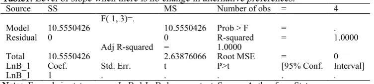
shows that when there is no change in the profile preference of individuals, the slope tends to 1. The effect here is therefore 1-1 = 0% as shown in Table-1.

Table1. Level of slope when there is no change in alternative preferences.

Source SS MS Number of obs = 4

F( 1, 3)=.

Model 10.5550426 10.5550426 Prob > F = .

Residual 0 0 R-squared = 1.0000

Adj R-squared = 1.0000

Total 10.5550426 2.63876066 Root MSE = 0

LnB_1 Coef. Std. Err. t P>t [95% Conf. Interval]

LnB_1 1 . . . . .

Notes: Formula in stata: regress LnB_1 LnB_1, noconstant. Source: Author from Stata.

From Table-2, the effect from introducing change in alternatives, leads to a slope of 0.6869. Meaning that the impact is 1 - 0.6869 = 0.3131. The impact of the change in 𝑆1 , due to the change in 𝑅2𝑁has a magnitude of 31 on a scale of 100.

Table 2. Level of slope when there is a change in alternative preferences.

Notes: Formula in stata: regress LnB_1 LnB_2, noconstant. Source: Author from Stata.

The shock had therefore a 31% impact on the aggregated behaviour of individuals.

Let us assume that we are in a stock market, the individual preferences are ordered according to their risk aversion (𝑅1𝑁). They therefore choose the

composition of their portfolio according to their risk aversion. After an exogenous short-term shock (drastic decline in oil prices, bad economic conditions, etc.) Individuals decide to change(𝑅2𝑁) the composition of their portfolios (increase their

investments in some assets and reduce in others).

The shock leading to (𝑅₂𝑁) has therefore an impact on individuals' risk aversion. The magnitude of that shock is 31 over the scale we’ve defined. This can be the market volatility or the market oversight. It has in this case, increased their aversion if y and x are risky assets (according to Graph. 1).

6. Conclusion

Finally, collective rationality in the aggregation of choices is sometimes difficult to establish. Arrow (1963) said that there was no voting rule that is not subject to bias. Thus, the impossibility theorem sets 4 conditions to be satisfied for any rational voting rule. The Borda rule respected 3 of them, but stumbled on the last one: Indifference of Irrelevant Alternatives.

By redesigning the Borda rule's weight determination technique and making it dynamic, this paper allows the rule to respect the Arrow IIA. The new rule is called Dynamic Borda Voting (DBV). The DBV also makes it possible to deal with the problem of cloning manipulation.

Calculations, propositions with proof and explanations are made to show the effectiveness of this method. From DBV, the paper presents a method to measure and quantify the magnitude of the shock due to change in irrelevant alternatives over a scale moving from 0 to 100.

3

These statistical regressions are only illustrative.

SS MS Number of obs = 4

F( 1, 3)= 178.43

Model 10.3805151 10.3805151 Prob > F = 0.0009

Residual .174527526 .058175842 R-squared = 0.9835

Adj R-squared = 0.9780

Total 10.5550426 2.63876066 Root MSE = .2412

LnB_1 Coef. Std. Err. t P>t [95% Conf. Interval]

References

Arrow, K.J. (1963). Social Choice and Individual Values. 2nd ed. Wiley.

Barbie, M., Puppe, C., & Tasnádi, A. (2006). Non-manipulable domains for the Borda count. Economic Theory, 27(2), 411–430. doi. 10.1007/s00199-004-0603-4

Béhue, V., Favardin, P., & Lepelley, D. (2009). La manipulation stratégique des règles de vote: Une étude expérimentale. Recherches économiques de Louvain, 75(4), 503-516. doi. 10.3917/rel.754.0503

Borda, J.C. (1781). Histoire de l'Académie Royale des Sciences. Mémoire sur les élections au scrutin. Condorcet, M.D. (1785). Éssai sur l’application de l’analyse à la probabilité des décisions rendues à

la pluralité des voix. Imprimerie Royale.

Dasgupta, P., & Maskin, E. (2003). On the Robustness of Majority Rule. Mimeo.

Diss, M., & Tlidi, A. (2016). Another Perspective on Borda's Paradox. GATE - Lyon Saint-Etienne WP No.1632. [Retrieved from].

Gibbard, A. (1973). Manipulation of votings schemes: A general result. Econometrica, 41(4), 587-601. doi. 10.2307/1914083

Islam, J., Mohajan, H., & Moolio, P. (2012). Borda voting is non-manipulable but cloning manipulation is possible. International Journal of Development Research and Quantitative Techniques, 2(1), 28–37.

Lehtinen, A. (2007). The Borda rule is also intended for dishonest men. Public Choice, 133(1-2), 73-90. doi. 10.1007/s11127-007-9178-5

Lepelley, D., Moyouwou, I., & Smaoui, H. (2017). Monotonicity paradoxes in three-candidate elections using scoring elimination rules. Social Choice Welfare. doi. 10.1007/s00355-017-1069-1

Maskin, E. (1995). Majority rule, social welfare functions, and game forms. in, K. Basu, P.K. Pattanik & K. Suzumura (Eds.), Choice, Welfare and Development. (pp.100-109), Oxford: Clarendon Press.

Saari, D., & McIntee, T. (2013). Connecting pairwise and positional election outcomes. Mathematical Social Sciences, 66(2), 140–151. doi. 10.1016/j.mathsocsci.2013.02.002

Satterthwaite, M.A. (1975). Strategy-proofness and Arrow’s conditions. Journal of Economic Theory, 10(2), 198-217. doi. 10.1016/0022-0531(75)90050-2

Copyrights