Identifying Sentiment Words
Using an Optimization-based Model without Seed Words
Hongliang Yu1, Zhi-Hong Deng2∗, Shiyingxue Li3
Key Laboratory of Machine Perception (Ministry of Education), School of Electronics Engineering and Computer Science,
Peking University, Beijing 100871, China
1[email protected] 2[email protected] 3[email protected]
Abstract
Sentiment Word Identification (SWI) is a basic technique in many sentiment analy-sis applications. Most existing research-es exploit seed words, and lead to low ro-bustness. In this paper, we propose a novel optimization-based model for SWI. Unlike previous approaches, our model exploits the sentiment labels of documents instead of seed words. Several experiments on re-al datasets show that WEED is effective and outperforms the state-of-the-art meth-ods with seed words.
1 Introduction
In recent years, sentiment analysis (Pang et al., 2002) has become a hotspot in opinion mining and attracted much attention. Sentiment analysis is to classify a text span into different sentiment polar-ities, i.e. positive, negative or neutral. Sentimen-t Word IdenSentimen-tificaSentimen-tion (SWI) is a basic Sentimen-technique in sentiment analysis. According to (Ku et al., 2006)(Chen et al., 2012)(Fan et al., 2011), SWI can be applied to many fields, such as determin-ing critics opinions about a given product, tweeter classification, summarization of reviews, and mes-sage filtering, etc. Thus in this paper, we focus on SWI.
Here is a simple example of how SWI is applied to comment analysis. The sentence below is an movie review in IMDB database:
• Boredperformers and a lacklusterplot and script, do not make agoodaction movie. In order to judge the sentence polarity (thus we can learn about the preference of this user), one must recognize which words are able to express senti-ment. In this sentence, “bored” and “lackluster” are negative while “good” should be positive, yet
∗Corresponding author
its polarity is reversed by “not”. By such analy-sis, we then conclude such movie review is a nega-tive comment. But how do we recognize sentiment words?
To achieve this, previous supervised approach-es need labeled polarity words, also called seed words, usually manually selected. The words to be classified by their sentiment polarities are calledcandidate words. Prior works study the re-lations between labeled seed words and unlabeled candidate words, and then obtain sentiment polar-ities of candidate words by these relations. There are many ways to generate word relations. The authors of (Turney and Littman, 2003) and (Kaji and Kitsuregawa, 2007) use statistical measures, such as point wise mutual information (PMI), to compute similarities in words or phrases. Kanaya-ma and Nasukawa (2006) assume sentiment word-s word-succeword-sword-sively appear in the text, word-so one could find sentiment words in the context of seed words (Kanayama and Nasukawa, 2006). In (Hassan and Radev, 2010) and (Hassan et al., 2011), a Markov random walk model is applied to a large word re-latedness graph, constructed according to the syn-onyms and hypernyms in WordNet (Miller, 1995). However, approaches based on seed words has obvious shortcomings. First, polarities of seed words are not reliable for various domains. As a simple example, “rise” is a neutral word most often, but becomes positive in stock market. Sec-ond, manually selection of seed words can be very subjective even if the application domain is deter-mined. Third, algorithms using seed words have low robustness. Any missing key word in the set of seed words could lead to poor performance. Therefore, the seed word set of such algorithms demands high completeness (by containing com-mon polarity words as many as possible).
Unlike the previous research work, we identi-fy sentiment words without any seed words in this paper. Instead, the documents’ bag-of-words
formation and their polarity labels are exploited in the identification process. Intuitively, polarities of the document and its most component sentimen-t words are sentimen-the same. We call such phenomenon as “sentiment matching”. Moreover, if a word is found mostly in positive documents, it is very like-ly a positive word, and vice versa.
We present an optimization-based model, called WEED, to exploit the phenomenon of “sentimen-t ma“sentimen-tching”. We firs“sentimen-t measure “sentimen-the impor“sentimen-tance of the component words in the labeled documents se-mantically. Here, the basic assumption is that im-portant words are more sentiment related to the document than those less important. Then, we estimate the polarity of each document using it-s component wordit-s’ importance along with their sentiment values, and compare the estimation to the real polarity. After that, we construct an op-timization model for the whole corpus to weigh the overall estimation error, which is minimized by the best sentiment values of candidate words. Finally, several experiments demonstrate the ef-fectiveness of our approach. To the best of our knowledge, this paper is the first work that identi-fies sentiment words without seed words.
2 The Proposed Approach
2.1 Preliminary
We formulate the sentiment word identification problem as follows. LetD={d1, . . . , dn}denote
document set. Vector⃗l=
l1 ...
ln
represents their
labels. If document di is a positive sample, then
li = 1; ifdi is negative, thenli =−1. We use the
notationC ={c1, . . . , cV}to represent candidate
word set, andV is the number of candidate words.
Each document is formed by consecutive words in
C. Our task is to predict the sentiment polarity of
each wordcj ∈C.
2.2 Word Importance
We assume each document di ∈ D is presented
by a bag-of-words feature vectorf⃗
i =
fi1 ...
fiV
,
wherefij describes the importance ofcj todi. A
high value of fij indicates word cj contributes a
lot to documentdi in semantic view, and vice
ver-sa. Note that fij > 0 if cj appears indi, while
fij = 0if not. For simplicity, everyf⃗i is
normal-ized to a unit vector, such that features of different documents are relatively comparable.
There are several ways to define the word importance, and we choose normalized TF-IDF (Jones, 1972). Therefore, we have fij ∝
T F−IDF(di, cj), and∥f⃗i∥= 1.
2.3 Polarity Value
In the above description, the sentiment polarity has only two states, positive or negative. We extend both word and document polarities to polarity val-ues in this section.
Definition 1 Word Polarity Value: For each word
cj ∈ C, we denote its word polarity value as
w(cj). w(cj) > 0indicatescj is a positive word,
whilew(cj) < 0indicatescj is a negative word.
|w(cj)|indicates the strength of the belief ofcj’s
polarity. Denotew(cj)aswj, and the word
polar-ity value vectorw⃗ =
w1 ...
wV
.
For example, ifw(“bad”)< w(“greedy”)<0, we
can say “bad” is more likely to be a negative word than “greedy”.
Definition 2 Document Polarity Value: For each documentdi,document polarity valueis
y(di) =cosine(f⃗i, ⃗w) =
⃗ fi
T
·w⃗
∥w⃗∥ . (1)
We denotey(di)asyifor short.
Here, we can regard yi as a polarity estimate
fordi based onw⃗. To explain this, Table 1 shows
an example. “MR1”, “MR2” and “MR3” are three movie review documents, and “compelling” and “boring” are polarity words in the vocabu-lary. we simply use TF to construct the document feature vectors without normalization. In the ta-ble, these three vectors,f⃗1, f⃗2 andf⃗3, are(3,1), (2,1)and(1,3)respectively. Similarly, we can get
⃗
w= (1,−1), indicating “compelling” is a positive
word while “boring” is negative. After normaliz-ingf⃗1,f⃗2andf⃗3, and calculating their cosine
“compelling” “boring”
MR1 3 1
MR2 2 1
MR3 1 3
[image:3.595.103.259.63.133.2]w 1 -1
Table 1: Three rows in the middle shows the fea-ture vectors of three movie reviews, and the last row shows the word polarity value vectorw⃗. For simplicity, we use TF value to represent the word importance feature.
2.4 Optimization Model
As mentioned above, we can regardyias a
polari-ty estimate for documentdi. A precise prediction
makes the positive document’s estimator close to 1, and the negative’s close to -1. We define the polarity estimate error for documentdias:
ei =|yi−li|=|
⃗ fi
T
·w⃗
∥w⃗∥ −li|. (2)
Our learning procedure tries to decrease ei. We
obtainw⃗ by minimizing the overall estimation
er-ror of all document samples ∑n
i=1
e2i. Thus, the
op-timization problem can be described as
min
⃗ w
n
∑
i=1
(f⃗i
T
·w⃗
∥w⃗∥ −li)
2. (3)
After solving this problem, we not only obtain the polarity of each wordcj according to the sign of
wj, but also its polarity belief based on|wj|.
2.5 Model Solution
We use normalized vector⃗xto substitute ∥ww⃗⃗∥, and
derive an equivalent optimization problem:
min
⃗
x E(⃗x) = n
∑
i=1
(f⃗i T
·⃗x−li)2
s.t. ∥⃗x∥= 1.
(4)
The equality constraint of above model makes the problem non-convex. We relax the equality constraint to∥⃗x∥ ≤1, then the problem becomes
convex. We can rewrite the objective function as the form of least square regression: E(⃗x) =
∥F ·⃗x−⃗l∥2, whereF is the feature matrix, and
equals to
⃗ f1
T
...
⃗ fn
T
.
Now we can solve the problem by convex op-timization algorithms (Boyd and Vandenberghe, 2004), such as gradient descend method. In each iteration step, we update⃗xby∆⃗x=η·(−∇E) = 2η·(FT⃗l−FTF⃗x), whereη >0is the learning
rate.
3 Experiment
3.1 Experimental Setup
We leverage two widely used document dataset-s. The first dataset is the Cornell Movie Review Data1, containing 1,000 positive and 1,000
nega-tive processed reviews. The other is the Stanford Large Dataset2 (Maas et al., 2011), a collection
of 50,000 comments from IMDB, evenly divided into training and test sets.
The ground-truth is generated with the help of a sentiment lexicon, MPQA subjective lexicon3.
We randomly select 20% polarity words as the
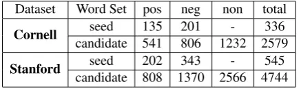
seed words, and the remaining are candidate ones. Here, the seed words are provided for the baseline methods but not for ours. In order to increase the difficulty of our task, several non-polarity words are added to the candidate word set. Table 2 shows the word distribution of two datasets.
Dataset Word Set pos neg non total Cornell candidate 541seed 135 201806 1232 2579- 336
Stanford candidate 808 1370 2566 4744seed 202 343 - 545
Table 2: Word Distribution
In order to demonstrate the effectiveness of our model, we select two baselines,SO-PMI (Turney and Littman, 2003) andCOM(Chen et al., 2012). Both of them need seed words.
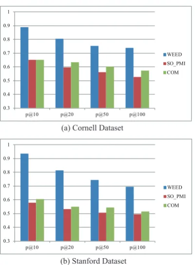
3.2 Top-K Test
In face of the long lists of recommended polarity words, people are only concerned about the top-ranked words with the highest sentiment value. In this experiment we consider the accuracy of the top K polarity words. The quality of a polarity word list is measured byp@K = Nright,K
K , where
Nright,K is the number of top-Kwords which are
correctly recommended.
1 http://www.cs.cornell.edu/people/pabo/movie-review-data/
[image:3.595.308.527.423.489.2]WEED SO-PMI COM
positive words negative words positive words negative words positive words negative words
great excellent bad stupid destiny lush cheapworst best great ridiculous bad perfect perfectly worst mess brilliant skillfully ridiculous annoying willstar plotevil
[image:4.595.74.529.61.149.2]terrific best boring ridiculous courtesycourtesy damn pathetic badfun stargarish true wonderfully awfulplot gorgeous magnificent inconsistenciesfool betterplot dreadfully stupid brilliant outstanding worse terrible temptationmarvelously desperate giddy lovehorror pretty fun
Table 3: Case Study
(a) Cornell Dataset
(b) Stanford Dataset 0.3
0.4 0.5 0.6 0.7 0.8 0.9 1
p@10 p@20 p@50 p@100
WEED
SO_PMI
COM
0.3 0.4 0.5 0.6 0.7 0.8 0.9 1
p@10 p@20 p@50 p@100
WEED
SO_PMI
COM
Figure 1: Top-K Test
Figure 1 shows the final result ofp@K, which
is the average score of the positive and negative list. We can see that in both datasets, our approach highly outperforms two baselines, and the preci-sion is14.4%-33.0%higher than the best baseline. p@10s of WEED for Cornell and Stanford
dataset-s reach to93.5%and89.0%, and it shows the top
10 words in our recommended list is exceptionally reliable. As the size ofK increases, the accuracy
of all methods falls accordingly. This shows three approaches rank the most probable polarity words in the front of the word list. Compared with the small dataset, we obtain a better result with large
Kon the Stanford dataset.
3.3 Case Study
We conduct an experiment to illustrate the char-acteristics of three methods. Table 3 shows top-10 positive and negative words for each method,
where the bold words are the ones with correc-t polaricorrec-ties. From correc-the firscorrec-t correc-two columns, we can see the accuracy of WEED is very high, where positive words are absolutely correct and negative word list makes only one mistake, “plot”. The oth-er columns of this table shows the baseline meth-ods both achieve reasonable results but do not per-form as well as WEED.
Our approach is able to identify frequently used sentiment words, which are vital for the applica-tions without prior sentiment lexicons. The sen-timent words identified by SO-PMI are not so representative as WEED and COM. For example, “skillfully” and “giddy” are correctly classified but they are not very frequently used. COM tends to assign wrong polarities to the sentiment words al-though these words are often used. In the5thand 6th columns of Table 3, “bad” and “horror” are
recognized as positive words, while “pretty” and “fun” are recognized as negative ones. These con-crete results show that WEED captures the gener-ality of the sentiment words, and achieves a higher accuracy than the baselines.
4 Conclusion and Future Work
We propose an effective optimization-based mod-el, WEED, to identify sentiment words from the corpus without seed words. The algorithm exploit-s the exploit-sentiment information provided by the docu-ments. To the best of our knowledge, this paper is the first work that identifies sentiment words with-out any seed words. Several experiments on real datasets show that WEED outperforms the state-of-the-art methods with seed words.
[image:4.595.82.283.183.456.2]Acknowledgments
This work is partially supported by National Nat-ural Science Foundation of China (Grant No. 61170091).
References
S. Boyd and L. Vandenberghe. 2004.Convex optimiza-tion. Cambridge university press.
L. Chen, W. Wang, M. Nagarajan, S. Wang, and A.P. Sheth. 2012. Extracting diverse sentiment expres-sions with target-dependent polarity from twitter. In
Proceedings of the Sixth International AAAI Confer-ence on Weblogs and Social Media (ICWSM), pages 50–57.
Wen Fan, Shutao Sun, and Guohui Song. 2011. Probability adjustment na¨ıve bayes algorithm based on nondomain-specific sentiment and evaluation word for domain-transfer sentiment analysis. In
Fuzzy Systems and Knowledge Discovery (FSKD), 2011 Eighth International Conference on, volume 2, pages 1043–1046. IEEE.
A. Hassan and D. Radev. 2010. Identifying text po-larity using random walks. In Proceedings of the 48th Annual Meeting of the Association for Compu-tational Linguistics, pages 395–403. Association for Computational Linguistics.
A. Hassan, A. Abu-Jbara, R. Jha, and D. Radev. 2011. Identifying the semantic orientation of foreign word-s. InProceedings of the 49th Annual Meeting of the Association for Computational Linguistics: Human Language Technologies, pages 592–597.
K.S. Jones. 1972. A statistical interpretation of term specificity and its application in retrieval.Journal of documentation, 28(1):11–21.
N. Kaji and M. Kitsuregawa. 2007. Building lexicon for sentiment analysis from massive collection of html documents. InProceedings of the joint confer-ence on empirical methods in natural language pro-cessing and computational natural language learn-ing (EMNLP-CoNLL), pages 1075–1083.
H. Kanayama and T. Nasukawa. 2006. Fully automat-ic lexautomat-icon expansion for domain-oriented sentiment analysis. InProceedings of the 2006 Conference on Empirical Methods in Natural Language Process-ing, pages 355–363. Association for Computational Linguistics.
Lun-Wei Ku, Yu-Ting Liang, and Hsin-Hsi Chen. 2006. Opinion extraction, summarization and track-ing in news and blog corpora. In Proceedings of AAAI-2006 spring symposium on computational ap-proaches to analyzing weblogs, volume 2001.
A.L. Maas, R.E. Daly, P.T. Pham, D. Huang, A.Y. Ng, and C. Potts. 2011. Learning word vectors for sen-timent analysis. InProceedings of the 49th annu-al meeting of the association for computationannu-al Lin-guistics (acL-2011).
Miller. 1995. Wordnet: a lexical database for english.
Communications of the ACM, 38(11):39–41.
B. Pang, L. Lee, and S. Vaithyanathan. 2002. Thumbs up?: sentiment classification using machine learn-ing techniques. InProceedings of the ACL-02 con-ference on Empirical methods in natural language processing-Volume 10, pages 79–86. Association for Computational Linguistics.