Intertemporal stability of survey based measures of risk and time preferences

Munich Personal RePEc Archive

Intertemporal stability of survey-based

measures of risk and time preferences

Drichoutis, Andreas C. and Vassilopoulos, Achilleas

Agricultural University of Athens, University of Ioannina

29 August 2016

Online at

https://mpra.ub.uni-muenchen.de/88237/

Intertemporal stability of survey-based measures of risk

and time preferences

∗

Andreas C. Drichoutis

and Achilleas Vassilopoulos

1

Agricultural University of Athens

2

University of Ioannina

3

ICRE8: International Center for Research on the Environment and the

Economy

First Draft: August 8, 2016

Abstract: Given the importance of risk and time preferences for economics and other disciplines, we seek to examine the intertemporal stability of six related survey-based mea-sures. Using a panel of subjects over three waves, between 2013 and 2015, we find remarkably high aggregate stability over the examined period in all six measures while we observe signif-icant patterns of instability at the individual level. Our results contribute to the discussion on the wider adoption of survey-based measures, especially considering the ease with which such measures can be incorporated in large-scale surveys.

Keywords: patience; impulsiveness; cognitive reflection test; DOSPERT.

JEL Classification: D80; D90.

∗_{This paper arises from an appendix questionnaire administered in parallel with the main questionnaire}

for the project EPHE - Epode for the Promotion of Health Equity- which has received funding from the European Union, in the framework of the Health Programme, agreement number: 2011 12 09. There is no other association of the results presented in this paper with EPHE.

†_{Assistant Professor, Department of Agricultural Economics & Rural Development, Agricultural}

Univer-sity of Athens, Iera Odos 75, 11855, Greece, e-mail: [email protected].

‡_{Assistant Professor, Department of Economics, University of Ioannina, University Campus, Ioannina,}

45110, Greece and ICRE8: International Center for Research on the Environment and the Economy, Ro-manou Melodou 3, 15125, Maroussi-Athens, Greece, e-mail: [email protected],[email protected].

1

Introduction

Economic theory suggests that the heterogeneity observed in decisions regarding retire-ment plans, occupational choices, insurance or other aspects of everyday life can be explained by differences in agents’ budget constraints as well as in their Risk and Time Preferences (RTPs). In addition, in almost all theories of economic behavior, utility functions are de-fined over goods, time periods and states of nature, placing RTPs at the crux of consumer behavior as traditionally studied in economics. Given that cost-benefit analysis calls for wel-fare calculations involving outcomes that are delayed or uncertain, policy recommendations should be always analyzed through the prism of these two concepts before they are put into action (Harrison et al., 2005).

In economic analysis, individual preferences are considered to be stable over time. Ander-sen et al. (2008) argue that the assumption of stable preferences lies in the ability to assign causation between changing opportunity sets and choices in comparative statics exercises or, in Stigler and Becker’s (1977) words, “no significant behavior has been illuminated by assumptions of differences in tastes”. For example, academics generalize observed choices among lotteries in the lab or in the field to build behavioral models and estimate risk param-eters. Similarly, professionals in the financial, insurance and health sector propose long-term products to their clients based on stated RTPs at the time of purchase. Implicitly, for these models/parameters or products to be of any use, stability of subjects or clients RTPs over their lifespan or period of investment is essential (Baucells and Villass, 2010). Otherwise, if individuals’ intertemporal trade-offs change over time, preference parameters have to be separately measured and accounted for in each time period (Meier and Sprenger, 2015). In the same spirit,Harrison et al.(2005) note that if preferences are volatile with respect to the passage of time, then researchers and policy-makers using out-of-sample predictions should worry about their conclusions. Aside individual invariance, aggregate stability of RTPs is also a very important concept in policy-making since, according to Meier and Sprenger (2015), if the aggregate distribution of behavior is unstable, then individual preference parameters will also exhibit such property. On the other hand, if choices over time are stable in the aggregate, then individuals’ plans and surveys may very well serve as tools in the pursuit of optimal policies in terms of social choice.

A number of methods have been proposed in the literature to measure RTPs. Risk pref-erences are often measured in controlled laboratory experiments, using standard procedures such as the elicitation of certainty or probability equivalents of lotteries through incentive-compatible mechanisms (e.g., the Becker, Degroot and Marshak (BDM) mechanism, first-and second-price auctions etc.) or the well-established methods proposed byHolt and Laury

(2002), Lejuez et al. (2002), Gneezy and Potters (1997) and Eckel and Grossman (2002, 2008). Analogously, typical measures of time preferences stem from experiments that either jointly elicit risk and time preferences (Andersen et al., 2008) using the multiple price list method (e.g., Coller and Williams, 1999), or Andreoni and Sprenger’s (2012) convex time budget (CTB). 1

However, lab experiments do have their limitations and thus, field and laboratory experi-ments should be treated as complementary tools in the evaluation of risk and time preferences (Andersen et al., 2010). Due to budget constrains, conducting large scale laboratory exper-iments to elicit preferences from representative samples is usually infeasible. Furthermore, although the methods presented above have been found to perform fairly well in predict-ing real life RTPs regardpredict-ing financial decisions, there is doubt on whether they generalize to important domains of life other than financial decision-making. For example, although present bias in an intertemporal choice task has been found to be associated with credit card debt and creditworthiness (Meier and Sprenger,2010,2012), savings behavior (Ashraf et al., 2006) and scholastic achievement (Mischel et al.,1989), Chabris et al. (2008) and Borghans and Golsteyn (2006) argue that experimentally elicited discount rates correlate only very weakly with health-related behavior such as exercising and smoking. In addition, Bradford et al. (2014) have found that elicited discount rates from incentivized tasks are only some-what predictive of self-reported time preferences measures, while they also show that using multiple self-reported proxies can better approximate association of time preferences with health, energy, and financial outcomes. Therefore, although we don’t have gold standard (i.e., incentivized) elicited time preferences measures, there is considerable value in studying the stability of survey based measures.

With respect to risk preferences, Barseghyan et al. (2011) andEinav et al. (2012) found that many individuals do not exhibit comparable degrees of risk aversion in different life domains, such as health, disability or car insurance while Deck et al. (2008) has suggested that this difference might be related to the instability of risk preferences across experimental tasks. Finally, Dreber et al. (2011) show that the risk taking among bridge players differed substantially between the domains of bridge and financial decision-making while MacCrim-mon and Wehrung(1990) argue that the risk attitudes of company managers appear to differ for risks in the recreational and financial domain. To this end, questionnaire-based measures of eliciting RTPs in the field and in various domains have witnessed a growing popularity in recent years (e.g., Dohmen et al., 2011). Thus, it is important to study, as we do in the present paper, whether survey based measures exhibit intertemporal stability and whether

1

For elaboration on these methods see Charness et al. (2013) and Drichoutis and Nayga Jr (2013); Andreoni et al.(2015) for risk and time preferences, respectively.

such measures can be used in place of incentivized measures, thus, making elicitation much more convenient and less resource intensive.

In this study, we examine the invariance of RTPs using primary longitudinal data on survey-based measures over a three-year course. To our knowledge, very few studies have evolved around the stability of RTPs using such measures in the relevant literature. In addition, our study is one of the very few that elicits preferences more than twice over the same subjects. To show how our study stands out with respect to the rest of the literature, we briefly review the literature in the next section (see particularly Tables1and 2). Finally, the span of our data is one of the the widest (T3−T1=2 years) while our sample size, even after two years of attrition, is at least comparable to many other studies using primary data. Echoing the literature on stability of RTPs we find aggregate stability of RTPs over the three-year course of our study. In addition, we find remarkable individual stability of most RTPs measures we employ over the same period while only a few of our measures show instability.

In the next section we survey the literature that examines stability of RTPs to set the context of our study. We present the details of our survey methods and sample characteristics in Section 3. Next, we present our analysis regarding temporal stability of RTPs at the aggregate and individual level. We conclude in the last section.

2

Literature review

Despite the importance of RTPs for economic research, the results regarding their stabil-ity are mixed. Below, we provide a list of published articles examining the stabilstabil-ity of time (Table 1) and risk (Table 2) preferences; we acknowledge of course that this list might be non-exhaustive. Note, that we have deliberately excluded studies using secondary data (e.g., Josef et al.,2016;Chuang and Schechter,2015;Niv et al.,2012;McGlothlin,1956) since the methods of measurement, the sample sizes as well as time lapses differ vastly not only with our study but with most studies that involve primary data collection in general. We have also included only studies that—like ours—examine time-invariance (in the terminology of Halevy, 2015). That is, we do not consider other types of time-stability such as consistency or stationarity (e.g., Horowitz, 1992; Gin´e et al., 2016; Li et al., 2013 or some treatments of Halevy, 2015).2,3 _{Finally, we exclude studies whose subjects were selected using criteria}

2

In the terminology of Horowitz (1992), intertemporal stationarity is similar to Halevy’s (2015) time-invariance but different than stationarity as defined inHorowitz(1992).

3

In Li et al. (2013), although the design would allow for tests of time-invariance, correlations across waves are not reported. However, it is stated that in the case of temporal discounting and loss aversion, common variance and substantial stability over 1 year is observed.

related to various medical disorders (e.g., Littlefield et al., 2015; Aklin et al., 2009; Bickel et al., 2011; Takahashi et al., 2007)4 _{and do not comment in the text about studies with} low participant numbers (although we do cite them in the respective tables just for sake of completeness).

2.1

Studies on time preferences

Interestingly, as shown in Table1, most articles regarding the stability of time preferences come from fields outside economics, such as psychology, decision science and neuroscience. All studies that are discussed below involved some kind of choice between sooner-smaller amounts and later-higher rewards; specific money and delay ranges are reported in Table1. In particular, Olson et al. (1999) report individual differences in children’s willingness to wait for a delayed reward that are relatively stable across 2-years’ time. Baker et al. (2003) examined stability of discount rates over a 1-week period for 30 current smokers and 30 never-before smokers with also high test-retest correlations while Johnson et al. (2007) replicated this study in a group of 30 light smokers with similar results.

In a very interesting study, Anokhin et al.(2011) offered subjects the same real choice at two different points in time, with a 2-year time lapse. Subjects were 606 12-year-olds from 303 pairs of mono-zygotic and di-zygotic twins who were re-tested at the age of 14. The choice was given individually to each twin who was unaware of their co-twin’s choice. They report a highly significant within-subject association between choices made at ages 12 and 14 but a significant decrease in the prevalence of impulsive choices with age. Finally, in one of the few relevant studies with more than 2 periods, Kirby (2009) collected choices with monetary incentives between sooner immediate and later rewards from student-subjects. The procedure was repeated after 5 weeks and 52 weeks thereafter. The common sample between periods 1-2, 2-3 and 1-3 was 81, 37 and 46, respectively. Their results indicate high temporal aggregate stability and suggest that the discount rate for monetary rewards is a stable individual trait. There are a few other studies that found individual stability but given small sample sizes, these will not be further discussed here (e.g. Simpson and Vuchinich, 2000;Ohmura et al.,2006; Kable and Glimcher, 2007;Peters and B¨uchel,2009). In the economics literature,Kirby et al.(2002), used a pool of 154 Tsimane’ Amerindians (10-80 years of age) and a series of incentive compatible choices over 4 quarters. Their results indicate that, starting from the second quarter and for both monetary and candy choices,

4

Of course, some could argue that nicotine dependence falls within this category and thusBaker et al.’s (2003) andJohnson et al.’s (2007) studies should also be excluded from the review. However, since nicotine dependence is quite common and might be also present in many other studies that do not control for it, we do not expect to have affected their results.

the correlations between the discount rates derived from consecutive periods are reliable (albeit low). Furthermore, excluding the first period, all rates were associated with a single underlying factor.5 _{W¨olbert and Riedl(2013) report both aggregate stability as well as high} test-retest correlations between the incentivized choices made by 53 student-subjects within an interval of 5 to 10 weeks. Dean and Sautmann (2014) and Meier and Sprenger (2015) found that aggregate choice profiles and corresponding estimates of discount parameters are unchanged over a period of one week and one year, respectively. They also report significant within-subjects rate correlations in their samples of 960 individuals in the former and 250 subjects in the latter study. Finally, Halevy (2015) used a sample of 130 student subjects to study various properties of time preferences including time-invariance. Unlike previous findings, his results suggest that average choices are inconsistent with the time invariance assumption since subjects are, on average, more impatient for a one week delay when asked at a later date. In addition, depending on the treatment, the amount of sooner payment and whether choices are interpreted as revealing strict or weak preference, the percentage of subjects that made time-invariant choices ranged from 44% to 68%.

2.2

Studies on risk preferences

The picture of risk preferences studies is quite different than time preferences. As seen in Table 2, the majority of studies regarding the inter-temporal stability of risk preferences comes from the economics literature while many studies have been conducted over the last few years indicating a rising interest. Levin et al. (2007) conducted a 3-year follow-up to 62 child-parent pairs from Levin and Hart’s (2003) study, repeating the real choice tasks between risky and safe options from the original study. Their results are supportive of both aggregate and individual stability in children and parents. Finally, Gl¨ockner and Pachur (2012) repeated all Holt and Laury (2002) tasks and several gain, loss and mixed lottery choice tasks in two sessions, a week apart. They found that in most of the cases, people made the same choice at the two sessions while the correlations of the prospect theory parameters showed a large effect size. Additional studies that employed small sample sizes will not be further discussed here (e.g. Ohmura et al.,2006; White et al., 2008) .

Within the economics literature, Wehrung et al. (1984) using hypothetical investment scenarios, investigated the stability of the Constant Relative Risk Aversion (CRRA) co-efficient over a 1-year period for 90 business executives and reported a small but highly significant positive correlation for the personal risk measures, but no stability for business risk propensity. Schoemaker and Hershey (1992) elicited CE for gains and losses from 160

5

AlthoughKirby et al.(2002) provide pair-wise correlation coefficients for rates across all periods, they do not discuss their statistical significance, nor perform aggregate comparisons.

MBA students and the same CE questions were administered 3 weeks later. Although some subjects were explicitly given monetary incentives to be consistent with their earlier answers ($10 for those in the highest decile in terms of consistency), test-retest correlations were low in both domains. Smidts (1997) examined long-run (1-year) risk attitudes concerning the market price for potatoes in 205 Dutch farmers. Using the midpoint chaining technique, he observes a strong correlation for the CRRA coefficient. Hey (2001) elicited preferences over 100 choices between pairwise risky lotteries made from 53 students and repeated over 5 periods that were separated by a few days from each other. During the 5 periods, a min-imum of 4 to a maxmin-imum of 91 consecutive changes in stated preferences were observed. Also, over all 5 waves, the number of differing answers within-subjects ranged from 3 to 48, indicating that on at least half the questions, subjects had fixed stated preferences. Harrison et al. (2005) tested the stability of CRRA coefficients at two points in time using the Holt and Laury (2002) procedure over 5-6 months and found no significant differences. The same procedure was followed by Andersen et al. (2008), but this time the lapses varied from 3 to 17 months. The CRRA coefficients were significantly correlated across time, although some variation was observed. In Goldstein et al. (2008), roughly 150 participants generated desired return distributions in hypothetical retirement savings scenarios in 2 sessions over a 1 year period (common sample was 85 subjects). Their results indicated that the transformed CRRA model-based risk parameters derived from the two different sessions were significantly correlated, especially when corrected for attenuation and investment experience.

Baucells and Villass(2010) on the other hand, concluded that albeit the statistical pattern among sessions was stable, there was a lot of instability in individual preferences across points in time. They used only two hypothetical lottery choice questions (one in the gain domain and 3 months later one in the loss domain) in 141 MBA student-subjects. Straznicka(2012) examined the 1-week stability of five different risk preference measures which all but one were of hypothetical nature. She observed an important stability of risk measures between sessions while at the individual level, the degree of risk aversion had significantly increased with the exception of survey-based measures that were found to be more stable. Zeisberger et al. (2012) elicited CE for gain, loss and mixed lotteries with real incentives from 73 students and observed considerable instability of risk aversion and probability weighting over a period of one month.

W¨olbert and Riedl (2013), using a series of choices between a sure amount and a lottery in 53 student-subjects which were repeated within 5 to 10 weeks, concluded that risk aversion and probability weighting parameter estimates revealed consistency both at the individual and the aggregate level. Finally, in L¨onnqvist et al. (2015), 44 student-subjects were called to make the same decisions in the incentivised Holt and Laury (2002) task within a time

interval of 13 to 15 months. The results suggest no robust test-retest stability for the lottery-choice measure. However, L¨onnqvist et al.’s (2015) design was very distinct because it also allowed the measurement of risk preferences from a risk taking questionnaire from the German Socio-Economic Panel (GSOEP). Unlike theHolt and Laury (2002) measure, these risk-related questions were found to have a very good test-retest stability.

Table 1: Literature on temporal stability of time preferences

Type of sample N at T1 N at T2 Common N Time lapse Methods Incentives

Olson et al.

(1999)

6-yo children 80 89 NA 2 years Choices between a single treat immediately available or a handful of treats later on Real

Simpson and Vu-chinich

(2000)

students 15 15 15 1 week

Choices between a standard larger later op-tion ($1,000) and a smaller immediate opop-tion. The magnitude of the sooner option (from $1 to $1000) was adjusted across trials until an indifference point was determined. Delay pe-riods range from 1 week to 25 years

Hypothetical

Kirby et al.

(2002)

10-80 year olds 154 ≈157

(same in T3&T4) 95-123 3 months

Choices between immediate monetary and food rewards and larger later rewards. Im-mediate rewards range from $b3.1 to $b8 (6 to 16 candies) and delayed from $b 7.5 to $b 8.5 (15 to 17 candies) for the monetary (food) treatment. Delays range from 7 to 157 days for both treatments

Monetary & food: 1 of the 8 mon-etary choices and 1 of the 7 candy choices were bind-ing

Baker et al.

(2003)

Heavy- and

non- smokers 60 60 60 1 week

Choices between a standard larger later op-tion of various magnitudes (e.g., $10, $100, and $1,000) and a smaller immediate option. The magnitude of the sooner option is adjusted across trials until an indifference point is de-termined. Delay periods range from 1 week to 25 years

Both monetary (1 random choice from $10 and $100 choices is binding) & Hypothetical

Ohmura et al.

(2006)

Students 22 22 22 3 months

Choices between a standard larger later op-tion of 100,000 yen and a smaller immediate option. The magnitude of the sooner option ranges between 100 and 100,000 yen. Delay periods range from 1 week to 25 years

Hypothetical

Johnson et al.

(2007)

Light smokers 30 30 30 1 week

Choices between a standard larger later op-tion of various magnitudes (e.g., $10, $100, and $1,000) and a smaller immediate option. The magnitude of the sooner option is adjusted across trials until an indifference point is de-termined. Delay periods range from 1 week to 25 years

Both monetary (1 random from $10 and $100 choices is binding) & Hypo-thetical

Kable and Glimcher

(2007)

Adults 12 12 (T3: 12)

12

(T3:12) 3 days-6 months

Choices between immediate reward of $20 and a larger delayed reward that varies randomly from $20.25 to $110. The delay ranges from 6 h to 180 d

Monetary: sub-jects are paid according to four randomly selected trials per session (except for the first session, which is hypothetical)

Continued on next page...

Table 1: Literature on temporal stability of time preferences (Cont.)

Type of sample N at T1 N at T2 Common N Time lapse Methods Incentives

Peters and B¨uchel

(2009)

Adults 22 22(short)

13(Long)

22(short) 13(Long)

Short≈4 days;

Long≈4 months

Choices between e_{20 available immediately}

and greater amounts at different delays or probabilities (not specified)

Monetary: 1 out

of 96 trails ran-domly selected as binding

Ballard and Knutson

(2009)

Adults 16 16 16 Not specified but short

Choices between $10 available immediately and greater amounts ($10.00, $10.50, $11.00, $13.00, $15.00, $20.00, $25.00) at different de-lays (0, 7, 30, 60, 90, 180 days)

Monetary: 1 out

of 84 trials

ran-domly selected

as binding in T1, same in T2

Kirby

(2009) Students 100

81 (T3:46) 81 (T1&T2&T3:37) T2-T1=5 weeks; T3-T2=1 year

Choices between immediate rewards and larger later rewards. Delays range from 7 to 186 days. Delayed rewards range from $25 to $85.

Monetary: one

subjects out of

every sessions is paid for one choice

Anokhin et al.

(2011)

12-yo twins 744 606 606 2 years Choice between $7 in cash immediately or $10

in 7 days

Monetary:

Deci-sion is binding

W¨olbert and Riedl

(2013)

Students 144 53 53 5-10 weeks

Choices between sooner rewards and later

re-wards. Smaller-sooner amounts range from

e11 toe54, and the larger-later amounts range

frome25 toe60. Delays range from 7 days to

200 days.

Monetary: 1

de-cision is randomly chosen as binding

Dean and Saut-mann

(2014)

Household

heads 969

965 (T3:961)

965

(T3:961) 1 week

Choices between sooner rewards and later

re-wards. Smaller-sooner amounts range from

CFA 50 to CFA 400, and the larger-later amount is CFA 300. Delay trade-offs are (A) now vs. next week and (B) next week vs. a week thereafter

Monetary: 1 deci-sion in each wave is randomly cho-sen as binding

Meier and Sprenger

(2015)

Subjects visit-ing tax assis-tance sites

890 794 203 ≈1 year

Choices between sooner rewards (that vary from $49 to $14) and a larger later reward set at $50. Time frame for sooner reward varies between now and 6 months. Time frame for later reward varies between 1 and 6 months.

Monetary: 10% of individuals is ran-domly paid one of their choices

Halevy

(2015)

First-year

Students 149 130 130 4 weeks

Choices between sooner rewards ($10 and $100) and MPLs with later rewards set at $9.9 to $11 and $99 to $110, respectively. Time frame for sooner reward is now and for later reward it is 1 week

Monetary: 1

student is paid

according to her

choices in the

$100 lottery and the rest according to those in the $10

one; 50-50% T1

or T2 decisions on these lotteries are binding

Notes: ‘N at T1’ and ‘N at T2’ stand for sample size at Time 1 and 2 respectively. ‘Common N’ is the sample size left after attrition at T2 or due to other constraints specified by the study. If preferences were elicited at a additional points, these are indicated as T3, T4 etc.

Table 2: Literature on temporal stability of risk preferences

Type of sample N at T1 N at T2 Common N Time lapse Methods Incentives

Wehrung et al.

(1984)

Senior

executives 500 90 90 1 year

Gain equivalences for investment decisions

in-volving personal and corporate resources Hypothetical

Love and Robison

(1984)

farmers 23 23 23 2 years Choices between pairs of distributions of

pos-sible after-tax income levels. Hypothetical

Schoemaker and Her-shey

(1992)

MBA Students 160 160 160 3 weeks Certainty equivalents for gain and loss lotteries

Monetary: $10 for consistency (top 10% of each group)

Smidts

(1997) Farmers 253 238 205 ≈1 year

Certainty equivalents for 50-50 lotteries where

the monetary amounts are prices for potatoes Hypothetical

Hey

(2001) Students 53 53

53

(also in T3,T4,T5) ≥2 days

100 choices between pairwise risky lotteries with various amounts (-$25, $25, $75 and $125)

Monetary: 1 out of 500 choice tasks is paid out

Harrison et al.

(2005)

Students 178 31 31 5-6 months Holt and Laury (2002) task Monetary

Ohmura et al.

(2006)

Students 18 18 18 3 months

Choices between a larger risky option of 100,000 yen (received with some probability) and a smaller but safe option. The magni-tude of the safe option ranged between 100 and 100,000 yen. Probability values of risky option ranged from .95 to .05

Hypothetical

Levin and Hart

(2003);

Levin et al.

(2007)

Students 72 62 62 3 years

Choices between a sure-thing option and a 50-50 or 20-80 risky choice both in the gain and the loss domains

Real: Partici-pants actually experience the consequences of their choices, either winning or losing dimes

Andersen et al.

(2008)

Representative sample of the adult Danish population

253 97 97 3-17 months MPL based onHolt and Laury(2002) task and iterated MPL

Monetary incen-tives: 10% chance of a randomly chosen task to be binding

Goldstein et al.

(2008)

Working

Adults 152 158 75 1 year

Participants use theSharpe et al.’s (2000) dis-tribution builder to generate desired return distributions in a fictitious retirement savings scenario

Hypothetical

Continued on next page...

Table 2: Literature on temporal stability of risk preferences (Cont.)

Type of sample N at T1 N at T2 Common N Time lapse Methods Incentives

White et al.

(2008)

Volunteers 39 39 39 2 weeks Balloon Analogue Risk Task (BART)

Monetary: Real payments based on outcomes of BART

Baucells and Villass

(2010)

MBA students 210 141 141 3 months Two lottery choice questions, one for gains and

one for losses Hypothetical

Gl¨ockner and Pachur

(2012)

Students 66 64 64 1 week

Holt and Laury(2002) task, several other gain, loss and mixed lottery choice tasks. Only 38 choice tasks are the same across Time 1 and Time 2.

Monetary incen-tives: 1 out of 138 choice tasks is paid out at a 100:1 exchange rate

Straznicka

(2012) Students 183 183 183 1 week

Evaluate riskiness of a gamble on a 0 to 10 scale, choose how much out of 100 to invest between a lottery and a risk free asset, cer-tainty equivalent of a lottery, rate willngness to take risks in financial decisions on a 0 to 5 scale,Holt and Laury(2002) task

Monetary: one choice from the

Holt and Laury

(2002) task is randomly chosen; all other tasks are hypothetical

Zeisberger et al.

(2012)

Students 86 86 73 1 month Certainty equivalents for gain, loss and mixed lotteries

Monetary: One subject every 10 subjects is paid out for a lottery outcome

W¨olbert and Riedl

(2013)

Students 144 53 53 5-10 weeks Choices between a sure amount and a lottery

Monetary: One decision is ran-domly chosen as binding

L¨onnqvist et al.

(2015)

Students 232 44 44 13-15 months

Holt and Laury (2002) task, Dohmen et al.

(2011) survey questions (evaluated on a 0 to 10 scale)

Monetary: one choice of the Holt and Laury (2002) task was paid out; the Dohmen et al. (2011) is non-incetivized

Notes: ‘N at T1’ and ‘N at T2’ stand for sample size at Time 1 and 2 respectively. ‘Common N’ is the sample size left after attrition at T2 or due to other constraints specified by the study. If preferences were elicited at a additional points, these are indicated as T3, T4 etc.

3

Methods

3.1

The Survey

To study the stability of RTPs, we chose to use a number of survey-based measures that pertain to patience, impulsiveness and risk (both financial and in other domains). All measures have been employed in previous studies and have been shown to correlate with the usual RTPs measures. Table 3 presents the specific questions and cites the sources of these measures which we briefly describe below.

Patience as a measure of the rate of time preferences has been validated as a survey measure in Vischer et al. (2013). In the same study, the authors draw the distinction of impatience with another measure, that of impulsiveness or impulsivity (the terms are used interchangeably in the literature). Impulsiveness is a psychological construct that is also thought to be closely related to intertemporal choice since the inability to delay gratification is considered the core problem of impulsive behaviors. Vischer et al. (2013) highlight that the distinction between impatience and impulsiveness is important, especially in situations where impulsive behavior may lead to decisions that are not in accordance with one’s time preferences. Both of these self-reported measures have been included in a large and repre-sentative data set, the German Socio-Economic Panel Study (GSOEP), for several years.

In addition, GSOEP includes two risk preferences measures. The first resembles the ones discussed above, in that it is a general measure of risk-taking propensity derived from a one-item survey question asking respondents to state their risk perception of themselves on a 0-10 scale. As simple as it may appear, this risk measure has been shown to be significantly related to actual risky behavior regarding investment in stocks, being self-employed, participating in sports, and smoking, even after controlling for a large number of observables (Dohmen et al.,2011). The answers to the second measure, called ‘the Risk investment question’ (also known as ‘the e_{100,000 question’) have been found to be strong predictors for decisions in}

the financial domain (Dohmen et al., 2011). On top of that, Leuermann and Roth (2012) reported a significant relationship between this lottery question and an incentivizedHolt and Laury(2002) risk preferences elicitation task.

For a non-unidimensional measure of risk, we opted for the Domain-Specific Risk-Taking (DOSPERT) scale (Weber et al., 2002). DOSPERT is a 40-item scale that assesses risk taking in five domains: financial decisions (F), health/safety (H/S), recreational (R), ethical, and social decisions. A shorter 30-item scale (Blais and Weber, 2006) has appeared in the literature as well as an ultra short 4-item scale (Coppola,2014) with good predictive validity. In this study, we took a middle point by adopting a limited (15-item) DOSPERT scale. To construct this limited scale, we started with the 30-item scale (Blais and Weber, 2006) and

eliminated the ethical and social subscales which were out of the scope of our research agenda. This left us with 18-items. We used 12 of these items in verbatim form (items 1-5, 8-9, 11-15 shown in Table 3) while we eliminated three questions: a) the unprotected sex question as inappropriate to address to parents (we discuss the characteristics of our sample in the next section), given the context of the rest of the questions which concerned the dietary habits of children b) two questions about investing in a diversified fund and business venture which we thought it would be difficult to explain given the ‘take home and return’ nature of our questionnaire. We replaced the ‘Drinking heavily at a social function’ (H/S domain) and ‘Going whitewater rafting at high water in the spring’ (R domain) with two questions from the limited DOSPERT scale of Szrek et al. (2012) (items 6 and 10 for the R and H/S domains, respectively; shown in Table 3). The remaining item ‘Betting a day’s income on the outcome of a sporting event’ was modified as ‘Betting 10% of your monthly income on the outcome of a sporting event’ since it is more common for people to think about income in monthly terms.

Finally, we have also included the well-known Cognitive Reflection Test (CRT) that has been shown to correlate well with a variety of risk and time preferences measures (Frederick, 2005). We do not test in our study whether there is actually a link between CRT and measures of risk/time preferences; we rather rely on the accumulated literature and focus here on the inter-temporal stability of the CRT measure. As a note, subjects did not receive any kind of feedback between waves.

3.2

Sample

A questionnaire consisting of all the above measures was delivered to schoolchildren aged 6-8 year old through two different schools in the city of Athens, Greece and during three measurement periods; baseline (T1:May-June 2013), after one year (T2:May-June 2014) and a year thereafter (T3:May-June 2015). The pupils were asked to deliver the questionnaire to their caretakers who, during two group-meetings with one of the researchers, had received an earlier notice and briefing about the purpose of the main study which was unrelated to this paper (discussed momentarily) as well as about the longitudinal nature of their responses. Because data collection was conducted through schools and in order to avoid confounding by social desirability or other such issues, we focused on ensuring the confidentiality of the responses. In particular, each school provided the unique register number (RN) of each student (but not their names); we gave back open envelopes that were labelled with the RN of the student to be handled and enclosed the questionnaires. When completed, the questionnaires were placed inside the same envelope by the respondents and the envelope

Table 3: Measures of risk and time preferences

Measure Question Measurement Reference

Patience Are you generally an impatient person, or someone who al-ways shows great patience?

0-10 scale Vischer

et al.

(2013) ImpulsivenessAre you generally an impulsive person, or someone who always

shows great caution?

0-10 scale Vischer

et al.

(2013) Risk Are you generally a person who is fully prepared to take risks

or do you try to avoid taking risks?

0-10 scale Dohmen

et al.

(2011) Risk

in-vestment

How much of a e_{100,000 prize would you invest in a lottery}

with a 50-50 chance of doubling it or losing half?

6 point scale ranging from

e_{100,000 to}

nothing with steps ofe_20,000

Dohmen

et al.

(2011); Leuer-mann

and Roth

(2012) Cognitive

Reflection Test

A bat and a ball cost e_{1.10 in total. The bat costs} e_1.00

more than the ball. How much does the ball cost?

Open ended Frederick (2005) If it takes 5 machines 5 minutes to make 5 widgets, how long

would it take 100 machines to make 100 widgets?

Open ended

In a lake, there is a patch of lily pads. Every day, the patch doubles in size. If it takes 48 days for the patch to cover the entire lake, how long would it take for the patch to cover half of the lake?

Open ended

DOSPERT 1. Going camping in the wilderness. (R) 1-7 scale Blais and Weber (2006); Szrek et al. (2012) 2. Betting a days income on lotto or scratch cards. (F)

3. Investing 5% of your annual income in a very speculative stock. (F)

4. Betting a days income at a high-stake poker game. (F) 5. Going down a ski run that is beyond your ability. (R) 6. Cool off in a fast-flowing river with shoulder-deep water on a hot summer day. (R)

7. Betting 10% of your monthly income on the outcome of a sporting event (F)

8. Driving a car without wearing a seat belt. (H/S) 9. Taking a skydiving class. (R)

10. Sit in the front seat of a car without a seat belt. (H/S) 11. Riding a motorcycle without a helmet. (H/S)

12. Sunbathing without sunscreen. (H/S) 13. Bungee jumping off a tall bridge. (R) 14. Piloting a small plane. (R)

15. Walking home alone at night in an unsafe area of town. (H/S)

was sealed and returned to the school; then sent by mail to the researchers. The same procedure was repeated over all waves. Thus, schools did not have access to the responses, since they were receiving and mailing closed envelopes, while we did not have access to the identities of the subjects. Aside the group-meetings, this procedure was also described in detail in the informed consent that children were asked to return signed by their parents, prior to the administration of the baseline questionnaires.

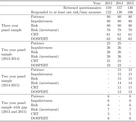
Table 4: Number of subjects per year and panel sample

Year: 2013 2014 2015 Returned questionnaires 159 157 130 Responded to at least one risk/time measure 122 130 106

Three year panel sample

Patience 80 80 80

Impulsiveness 80 80 80

Risk 80 80 80

Risk (investment) 78 78 78

CRT 61 61 61

DOSPERT 62 62 62

Two year panel sample

(2013-2014)

Patience 25 25

-Impulsiveness 26 26

-Risk 26 26

-Risk (investment) 26 26

-CRT 21 21

-DOSPERT 23 23

-Two year panel sample

(2014-2015)

Patience - 15 15

Impulsiveness - 15 15

Risk - 15 15

Risk (investment) - 14 14

CRT - 11 11

DOSPERT - 12 12

Two year panel sample with gap (2013 and 2015)

Patience 6 - 6

Impulsiveness 6 - 6

Risk 6 - 6

Risk (investment) 7 - 7

CRT 5 - 5

DOSPERT 6 - 6

The purpose for choosing the specific sample is that our questionnaire was an appendix to that of an unrelated main questionnaire which collected various data regarding the socio-economic characteristics of the parents and the dietary, sedentary and sleeping behavior of the child as well as other family-environmental variables. This questionnaire allowed the identification of the respondent (in terms of his/her relation to the child) and thus we were

able to perform individual matches in the measures of RTPs across waves. The selection of schools was made to serve the critical requirements of the main survey which was to assure the recruitment of families with both higher and lower socio-economic status but without worrying too much about the differences in ethnicity/culture. Although the main survey took place in seven European countries, the appendix questionnaire with RTPs measures was only administered to Athens, Greece. Results from analysis of the main questionnaire (which is unrelated to RTPs) along with details on the design and methodology of the survey are described elsewhere (Mantziki et al.,2014).

Respondents were asked to return the questionnaires in two-weeks’ time. Response rates were high, reaching 88.3% in the first year, 87% in the second year and 72.2% in the third year. However, as Table 4 shows, about 80% of the returned questionnaires contained only partially completed RTPs answers, lowering the actual response rates to 59%-72%. In terms of follow-up rates, the number of matched responses in all three waves ranges from sixty-one to eighty subjects, depending on the specific measure. Finally, depending on the specific measure, five to twenty-six respondents were only tracked in two out of the three points in time. We do not analyze data points related with the two-year panel at T1 and T3 (bottom panel of Table 4) due to very small number of observations.

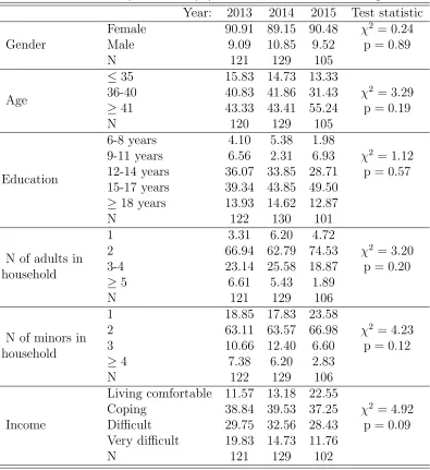
In terms of demographics, respondents are mostly female, older than the age of 36 years old and of medium to high education level (Table 5). They mainly live in households with 2 to 4 adults and 1 or 2 children. As per income status, half of the respondents self-reported to be in the lower classes while the other half in the higher ones. This profile was of course to be expected, considering the target audience that were primary caretakers of 6- to 8-year old children in both high and low socio-economic-status families. Overall, although our sample is far from representative of the general population, it is comparable to most other studies presented above. Like many other studies that use students as their research population, we do not claim external validity to the general population but only a contribution to the realm of studies dealing with stability of RTPs. We do claim, however, that the time span of our study is one of the longest in the literature

4

Results

Results are presented in the following sections. First, aggregate response profiles over the three years of the study are presented for each of the risk and time preferences measures. Second, we restrict our attention to the three year panel sample in order to examine their temporal stability at the individual level. We also examine temporal stability of responses from the two year panel sample, that is, for subjects that participated in years 2013-2014 or

Table 5: Summary statistics (%) for 2013, 2014 and 2015 samples Year: 2013 2014 2015 Test statistic

Gender

Female 90.91 89.15 90.48 χ2 = 0.24

Male 9.09 10.85 9.52 p = 0.89

N 121 129 105

Age

≤35 15.83 14.73 13.33

36-40 40.83 41.86 31.43 χ2 = 3.29

≥41 43.33 43.41 55.24 p = 0.19

N 120 129 105

Education

6-8 years 4.10 5.38 1.98

9-11 years 6.56 2.31 6.93 χ2 = 1.12

12-14 years 36.07 33.85 28.71 p = 0.57

15-17 years 39.34 43.85 49.50

≥18 years 13.93 14.62 12.87

N 122 130 101

N of adults in household

1 3.31 6.20 4.72

2 66.94 62.79 74.53 χ2 = 3.20

3-4 23.14 25.58 18.87 p = 0.20

≥5 6.61 5.43 1.89

N 121 129 106

N of minors in household

1 18.85 17.83 23.58

2 63.11 63.57 66.98 χ2 = 4.23

3 10.66 12.40 6.60 p = 0.12

≥4 7.38 6.20 2.83

N 122 129 106

Income

Living comfortable 11.57 13.18 22.55

Coping 38.84 39.53 37.25 χ2 = 4.92

Difficult 29.75 32.56 28.43 p = 0.09

Very difficult 19.83 14.73 11.76

N 121 129 102

Notes: The ‘test statistic’ column displays Pearson’s chi-squared test (and cor-responding value) for Gender and Kruskal-Wallis tests (and corcor-responding p-values) for all the other variables. Sample is constrained to subjects that have non-missing values for at least one of the risk/time measures.

2014-2015.

4.1

Temporal stability in aggregate

In this section we examine stability of preferences by looking at the aggregate distribution of responses for each risk/time preferences measure. We examine responses for all subjects that responded to at least one of the risk/time measures (sample size for each year is given

in second row of Table 4); we do not restrict analysis to the panel sample. This is justified by the fact that sample pools are similar across the three years of the study as shown in Table 5.

Figure 1plots distributions of responses by year, separately for each risk/time measure. Distributions of responses are depicted in the form of histograms with percentage of responses on the vertical axis. The only exception is the DOSPERT measure which, given the wide range of scores, it is depicted with a kernel density plot.6 _{Eyeballing Figure 1 reveals a} consistent pattern of responses across years with just a few exceptions here and there. What matters for aggregate stability, however, is not a few differences in the scale of a measure but the overall distribution of responses.

Table 6shows mean, standard deviation and median for each risk/time preferences mea-sure and their subscales. Summary statistics provide some, albeit incomplete, information about the underlying distribution of the data. For example, looking at the median, we see that there are just small shifts in the location of the distributions from one year to the other. Statistical tests can inform us whether two samples are drawn from the same popu-lation. Typically, Kolmogorov-Smirnov (KS) tests (Kolmogorov(1933), reprinted in English byShiryayev(1992);Smirnov(1948)) and Wilcoxon-Mann-Whitney rank-sum (WMW) tests (Wilcoxon, 1945; Mann and Whitney, 1947) are employed to test whether the underlying distributions of the two samples are equal. The WMW test detects only locational shifts while the KS detects differences in distributions due to location, scale, or family. A drawback of the KS test for our case, is the assumption that the data are drawn from a continuous distribution, while most of our risk/time measures are discrete and ordinal in nature. An alternative to the KS test is the Epps-Singleton test, where both continuous and discrete data may be used and has been shown to be more powerful than the KS test (Epps and Singleton, 1986).7

The last two columns of Table 6show results for: a) the Epps-Singleton test for the Pa-tience, Impulsiveness, Risk and Risk/investment measures b) the KS test for the DOSPERT measure and its subscales c) the WMW test for the CRT and d) proportion tests for the CRT individual questions (CRT1, CRT2 and CRT3). As shown, most of the tests fail to

reject the null that the underlying distributions of the two samples are equal. There is one minor exception for the CRT2 and CRT3 questions when looking at the change between 2014

and 2013. However, the statistical significant results fail to show up in the aggregate CRT measure.8

6

Figure A1 in Apendix A shows additional graphs for the DOSPERT subscales and the individual questions of the CRT.

7

SeeGoerg and Kaiser(2009) for a Stata implementation. 8

In FigureA1eand A1fit appears that less subjects give a wrong answer to these two particular CRT

Table 6: Descriptive statistics per year

2013 2014 2015 2013 vs. 2014 2014 vs. 2015

Mean S.D. Median Mean S.D. Median Mean S.D. Median Statistic p Statistic p Patience 6.64 2.30 7.00 6.74 2.39 7.00 6.53 2.26 7.00 W2 =3.58 0.47 W2 =1.94 0.75

Impulsiveness 5.07 2.39 5.00 5.67 2.37 6.00 5.42 2.54 5.00 W2 =5.32 0.26 W2 =6.87 0.14

Risk 5.23 2.49 5.00 5.25 2.15 5.00 4.66 2.43 5.00 W2 =4.17 0.38 W2 =6.65 0.16

Risk (investment) 5.28 0.95 6.00 5.12 0.95 5.00 5.10 1.01 5.00 W2 =3.83 0.43 W2 =3.68 0.45

DOSPERT 35.50 13.79 32.50 36.08 14.11 33.00 36.05 14.77 33.00 D= 0.09 0.73 D=0.08 0.85 DOSPERT-f 8.79 4.51 8.00 9.22 4.55 8.00 8.73 4.51 8.00 D=0.09 0.61 D=0.08 0.88 DOSPERT-h/s 12.94 6.81 11.00 13.33 6.97 11.00 13.31 7.28 12.00 D=0.10 0.50 D=0.12 0.34 DOSPERT-r 13.77 7.62 12.00 13.44 7.97 11.00 13.96 7.86 13.00 D=0.08 0.74 D=0.11 0.46 CRT 1.08 1.16 1.00 1.35 1.21 1.00 1.41 1.19 1.00 Z =-1.72 0.09 Z =-0.34 0.73 CRT1 0.25 0.43 0.00 0.29 0.46 0.00 0.30 0.46 0.00 Z =-0.72 0.47 Z =-0.17 0.86

CRT2 0.37 0.48 0.00 0.50 0.50 0.50 0.50 0.50 0.50 Z =-2.09 0.04 Z =0.00 1.00

CRT3 0.41 0.49 0.00 0.54 0.50 1.00 0.57 0.50 1.00 Z =-1.90 0.06 Z =-0.49 0.63

Notes: f stands for the Domain-Specific Risk-Taking scale on the financial domain, h/s is for the health/safety domain, DOSPERT-r is foDOSPERT-r the DOSPERT-recDOSPERT-reational domain. TheiDOSPERT-r sum composes the DOSPERT scale. CRT1, CRT2 and CRT3 stand for the three components of the Cognitive

Reflection Test (CRT). ‘Statistic’ columns show the W2 statistic of the EppsSingleton test, the D statistic of the Kolmogorov-Smirnov test, and the

Z-statistic for the Wilcoxon-Mann-Whitney test (CRT variable) and proportion tests (CRT1, CRT2, CRT3 variables). The ‘p’ column shows p-values

for the respective calculated statistics.

(a) Percentage distribution of patience scale (b) Percentage distribution of impulsiveness scale

(c) Percentage distribution of willingness to take risks scale

(d) Percentage distribution of lottery investment question

(e) Kernel density of Domain-Specific Risk-Taking scale

(f) Percentage distribution of number of correct answers in the Cognitive Reflection Test

Figure 1: Distribution of responses across years for the risk/time measures

All in all, the analysis in this section echoes the results from the literature about aggregate stability of risk and time preferences. This should not downplay the importance of our results since they concern preference stability over a wide time frame of three consecutive years, one of the largest in the literature. Although aggregate preference stability is important, Meier and Sprenger (2015) note that a stable distribution of responses could be obtained without individual stability. Next section tackles the issue of individual level stability of preferences by analyzing only the panel samples.

4.2

Temporal stability in individual behavior

Given the voluntary nature of responding to the questionnaire and the three time points at which the questionnaires were filled, we ended up with two types of panels. In the first panel, we have individuals that respondent to all three waves of the survey. Table 4 shows that the number of subjects which have complete responses in all three waves for each risk/time measure varies from 61 subjects (for CRT) to 80 subjects (for Patience, Impulsiveness and Risk). These numbers are reduced even further if one tries to combine responses to the risk/time measures with demographics, since a few more subjects have incomplete information regarding one or more demographic variables.

One way to analyze data from the three year panel is to calculate the difference between values in two consecutive years.9 _{A person with stable responses in the two years should have} a score of differences equal to zero. Subjects with instability would deviate from zero, so that larger differences would indicate greater instability. Figure2shows scatter graphs of changes in year 2014 with respect to 2013 (horizontal axis) and changes in year 2015 with respect to 2014 (vertical axis). Points that fall exactly on the dashed cross lines intersection, that is, on coordinates [0,0], indicate subjects with (deterministic) response stability for the full three year period. To get a sense of proportions, marks are depicted as bubbles with bubble sizes proportional to the frequency of occurrence of each case.10 _{Bubbles that fall on either} the vertical or the horizontal dashed cross lines, show subjects that gave the same response in at least two time points.11 _{By looking at the graphs in Figure 2 one can see that there}

questions in 2014 as compared to 2013 which is what the statistical test might be picking up. 9

Since most of our RTPs measures are ordinal in nature, taking their difference does not ensure the ordinality of the resulting measure nor it is permissible to make interpretations in continuous terms. Thus, we do not use this technique for conducting statistical tests or econometric analysis but rather as a trick to graph stability of responses.

10

To illustrate this, consider Figure2awhich depicts the Patience scale. This figure shows that 18 subjects fall exactly on the cross intersection which is to say that 18 subjects gave the exact same response on the Patience scale in the three years of the survey.

11

Consider Figure2aagain. The figure shows 15 (=7+5+2+1) subjects on the horizontal cross line and 12 (=2+1+2+3+2+1+1) subjects on the vertical cross line. These subjects gave the exact same response on the patience scale in two time points. These are different subjects than the 18 subjects that fall on the

is some heterogeneity in terms of stability of responses. However, there are enough subjects that fall on either one of the cross dashed lines, which indicates stability of preferences for at least two time points. The percent of subjects that fall on either one of the dashed cross lines is quantified in TableA1in AppendixAand can be as high as 80.8% of subjects for the Risk/investment measure or as low as 27.4% for the CRT. This indicates large variability between risk/time measures in terms of their temporal stability for the three year panel sample.

4.3

Stochastic Models

The analysis above is, of course, deterministic in that it allows no error in the decision making process. To account for the panel data structure, we explore individual stability by means of random parameters regressions. However, given that fixed and random effects panel regressions estimate population averages and not population distributions, we esti-mate random parameters (RP) ordered logit models (using maximum simulated likelihood methods) for the Patience, Impulsiveness, Risk and Risk/investment measures and RP linear regression models for DOSPERT and CRT. Since RP models assume that parameters are distributed with a mean (provided by the deterministic component) and a stochastic compo-nent, to test for aggregate stability we are mainly interested in the coefficient estimates of the year dummies while for individual stability, we focus on the parameters of their distributions (the values of σ). The results are shown in Table 7 while Table A2 in Appendix A shows results for the DOSPERT subscales and CRT individual questions. The upper panel shows results without any demographic control variables included in the model specification while the lower panel includes as controls the set of demographic variables shown in Table 5. Ta-ble 7 omits estimated parameters for ancillary parameters and coefficients for demographic controls in order to focus attention to the year dummies (the year 2014 serves as the base category) and their respective scale parameters.

Table7shows that for all measures, none of the year dummies is statistically significant in both panels of the table (with and without demographic controls), indicating high aggregate temporal stability of these measures. On the other hand, the scale parameters for the distributions of random parameters show a consistent pattern of statistical significance for all but the CRT measure, indicating instability of these measures at the individual level.

The second type of panel concerns subjects that responded to two consecutive waves but

cross intersection. Table A1in Appendix A depicts the number and percent of subjects that fall on the intersection of the dashed cross lines, on either one of the cross lines and the cumulative percent. As shown in TableA1, if we use the cumulative percent as the desired metric, highest individual stability is achieved by the Risk/investment measure, followed by the DOSPERT measure, while the least stable measure is the CRT.

(a) Changes in Patience scale (b) Changes in Impulsiveness scale

(c) Changes in Risk scale (d) Changes in Risk/investment question

(e) Changes in the Domain-Specific Risk-Taking scale

(f) Changes in number of correct answers in the Cognitive Reflection Test

Figure 2: Scatter graph of changes for the risk/time measures for the three year period weighted by frequency

Notes: In each graph, the horizontal axis shows differences in scores for 2014 vs. 2013. The vertical axis shows differences for 2015 vs. 2014. Marks that fall on the cross in each graph indicate subjects that showed stability of the respective measure (i.e., the score difference is exactly zero) for at least a one year time lapse. Marks that fall exactly on the cross intersection show subjects that are consistent in their responses for all three years. Bubble size is proportional to the frequency of each. A small number near the bubble indicates the frequency of each case. Bubbles with no numbers are single cases. Given the wide range of the DOSPERT scale, data are grouped in intervals of range of five (the first category being the [-2,2]) to allow small deviations from one year to the other to be classified as consistent. That is, any particular bubble for the DOSPERT scale counts observations within a range and not on a specific data point.

Table 7: Random parameters ordered logit and linear regression for the three year panel sample Patience Impulsiveness Risk Risk investment DOSPERT CRT

w

/o

d

em

og

ra

p

h

ic

s _{Constant 4.484}∗∗∗ _4.408∗∗∗ _3.802∗∗∗ _37.333∗∗∗ _36.758∗∗∗ _1.426∗∗∗ 2013 -0.307 -0.782∗ _{0.281 0.349 -0.827 -0.244}

σ2013 0.276 0.491∗∗ 1.229∗∗∗ 0.992∗∗∗ 3.985∗∗ 0.243

2015 -0.109 -0.523 -0.516 -0.016 -1.491 -0.114

σ2015 0.554∗∗∗ 1.107∗∗∗ 1.187∗∗∗ 0.504∗∗ 7.651∗∗∗ 0.041

N 240 240 240 234 186 183

Log-L -481.240 -486.379 -443.535 -275.023 -751.943 -284.794

w

/

d

em

og

ra

p

h

ic

s Constant 7.153∗∗∗ _7.207∗∗∗ _7.400∗∗∗ _37.601∗∗∗ _48.263∗∗∗ _1.294∗∗ 2013 -0.301 -0.979∗ _{0.267 0.773 -0.719 -0.170}

σ2013 0.591∗∗ 0.533∗∗ 1.465∗∗∗ 1.888∗∗∗ 0.348 0.112

2015 -0.214 -0.458 -0.552 0.224 -2.999 -0.228

σ2015 0.879∗∗∗ 1.301∗∗∗ 1.488∗∗∗ 1.002∗∗∗ 3.362∗∗ 0.549∗∗∗

N 213 213 213 207 171 165

Log-L -399.563 -417.857 -390.632 -226.657 -668.548 -227.219

Notes: Random parameters ordered logit models are estimated for Patience, Impulsiveness, Risk and Risk investment. Random parameters linear regression models are estimated for DOSPERT and CRT. Allσ _{are estimates of random parameters’ standard deviations assuming a normal} distri-bution for the year dummies and fixed coefficients for the rest or independents. Ancillary parameter estimates are omitted. The lower panel of the table shows results from models including demographic controls shown in Table5. Coefficient estimates for demographic controls are omitted. * p<_{0.1, **} p<_{0.05, *** p}<_0.01.

not in the third one. These are subjects with responses at time points 2013-2014 and 2014-2015. The number of subjects that responded to each of the risk/time measures is shown in the third and fourth panels of Table 4. We pool together responses from both two year panels in order to maximize available sample size. Table 8 shows the percent of subjects that exhibited stability in their responses in the two consecutive years of the survey. As shown, the Risk/investment measure exhibits very high stability for 57.5% of subjects. The least stable measures are the overall DOSPERT measure, followed closely by Patience and Impulsiveness.

In Table9we show results from random parameters ordered logit and random parameters linear regressions where the respective risk/time preferences measure of interest is regressed on a year dummy taking the value of 1 for the second year of the two year panel.12 _The upper panel shows results without any demographic control variables while the lower panel includes as controls the set of demographic variables shown in Table 5. Table 9 omits estimated parameters for ancillary parameters and coefficients for demographic controls. In both panels of Table 9 none of the year dummies is statistically significant, showing again aggregate stability over a one-year period. In terms of individual stability, the Implulsiveness,

12

Table A3in AppendixAshows results for the DOSPERT subscales and CRT individual questions.

Table 8: Percent of subjects showing stability/instability for the two year panel sample

Stability Instability

Patience 30.00 70.00

Impulsiveness 31.71 68.29

Risk 41.46 58.54

Risk (investment) 57.50 42.50

DOSPERT 28.57 71.43

DOSPERT-f 55.26 44.74

DOSPERT-h/s 35.00 65.00

DOSPERT-r 36.84 63.16

CRT 53.13 46.88

CRT1 83.78 16.22

CRT2 67.57 32.43

CRT3 73.53 26.47

Notes: For the DOSPERT measure, data are grouped in intervals of range of five to allow small deviations from one year to the other to be classified as consistent. Given the narrower range of the DOSPERT subscales, data are grouped in intervals of range of three for DOSPERT-f, DOSPERT-h/s and DOSPERT-r.

Risk and DOSPERT measures show instability as the distribution parameters of the second-year dummy is significant. In Patience and CRT, there is some indication of temporal instability but the conclusion changes, depending on whether we control for demographics, so this result is not clear-cut.

Given that we analyzed separately the three year and two year panels, one might worry for robust statistical inference with respect to reduced sample sizes. In Table A4 and Table A5 in the Appendix A we show additional results for the main risk/time measures and their subscales, respectively, where we pool together the three year panel and the two year panel. Results echo what was discussed above in that we can safely assume temporal stability at the aggregate but a general individual instability, with the exception of the CRT measure.

5

Conclusions

Despite the noise and the absence of real incentives for truthful answers, using survey-based measures of RTPs is of paramount importance for researchers since survey-survey-based mea-sures make elicitation much more convenient and less resource intensive. In this paper, we investigated the empirical power of a questionnaire consisting of survey-based measures, in an effort to learn more about the stability of these concepts that are crucial in economic re-search. To do so, we analysed patterns of aggregate differences as well as of individual-level changes in six measures of RTPs.

Table 9: Random parameters ordered logit and linear regression for the two year panel samples

Patience Impulsiveness

Risk

DOSPERT

CRT

w

/o

d

em

o-gr

ap

h

ic

s

Constant

4.101

2.282

3.476

35.000

1.313

2nd year

-0.081

0.012

-0.068

1.098

0.372

σ

1.251

1.035

0.430

9.704

0.211

N

80

82

82

70

64

Log-L

-169.404

-181.779

-166.752

-284.515

-102.924

w

/

d

em

o-gr

ap

h

ic

s

Constant

6.740

0.318

13.149

23.744

-0.916

2nd year

- 0.175

-0.159

-0.306

2.055

0.373

σ

0.06

-0.954

1.227

11.410

0.638

N

78

80

80

68

64

Log-L

-149.655

-163.796

-161.294

-268.595

-76.526

Notes: Random parameters ordered logit models are estimated for Patience, Impulsiveness, Risk and Risk investment (did not converge, due to insufficient variability). Random param-eters linear regression models are estimated for DOSPERT and CRT. Ancillary parameter estimates are omitted. The lower panel of the table shows results from models including demographic controls shown in Table 5. Coefficient estimates for demographic controls are omitted. * p<_{0.1, ** p}<_{0.05, *** p}<_0.01.

In line with existing literature, we observe temporal stability of RTPs measures at the aggregate level. This is extremely useful in policy-making where the allocation of resources should be based on the interest of the groups and not of the individuals. Even if agents move between groups throughout the implementation of a designed policy, the allocation may still be optimal if group interests remain stable. At the individual level, our results reveal that there is heterogeneity in terms of stability with only one of the measures (CRT) showing signs of intertemporal stability while all others fail to do so.

Aside the importance of our findings, we acknowledge a number of limitations related to our study. First of all, the profile of our respondents is very specific and cannot be considered as representative of the general population. However, there is little evidence suggesting that the results could be completely driven by differences in the pool of respondents; a fact that is also the cornerstone of the validity of lab experiments, that usually involve student-subjects (Belot et al., 2010).

Second, as with all survey-based measures, our approach does not provide respondents with incentives to reveal their preferences. In addition, since we do not have data on actual behavior with respect to risky or intertemporal choices, we cannot establish links between RTPs, as measured by the employed survey instruments, with real choices in the field; for this, we have to rely on previous studies. Also, as Harrison et al. (2005) note, the stability

over longer periods of time requires that one take into account possible changes in the ‘states of nature’. While we do record possible changes in states of nature, we do not know for sure whether we have recorded every possible change. Thus, whether our results point towards the (in)stability of the behavioral concepts we seek to examine or toward measurement error, is a question that we cannot be extremely confident about. The inclusion of questions like the ones we have employed in our study, in large longitudinal surveys that allow their observation over time in conjunction with other behavioral patterns and characteristics of respondents, is definitely a step towards the right direction; data stemming from such sources are valu-able for the study of preference stability. Judging from the recent flourishing literature on intertemporal stability of such data, we feel that this is a direction currently well-understood by economists, psychologists and other social and behavioral scientists. Finally, like many other longitudinal surveys, our study does not address sample selection and attrition effects. This requires much more elaborate experimental designs and methods and, consequently, are scarcely used (e.g., Harrison et al.,2014, for one of a few exceptions).

References

Aklin, W. M., M. T. Tull, C. W. Kahler, and C. Lejuez (2009). Risk-Taking Propensity Changes Throughout the Course of Residential Substance Abuse Treatment. Personality and individual differences 46(4), 454–459.

Andersen, S., G. W. Harrison, M. I. Lau, and E. Elisabet Rutstrm (2008). Lost in state space: Are preferences stable? International Economic Review 49(3), 1091–1112.

Andersen, S., G. W. Harrison, M. I. Lau, and E. E. Rutstr¨om (2008). Eliciting risk and time preferences. Econometrica 76(3), 583–618.

Andersen, S., G. W. Harrison, M. I. Lau, and E. E. Rutstr¨om (2010). Preference heterogene-ity in experiments: Comparing the field and laboratory. Journal of Economic Behavior and Organization 73(2), 209–224.

Andreoni, J., M. A. Kuhn, and C. Sprenger (2015). Measuring time preferences: A com-parison of experimental methods. Journal of Economic Behavior & Organization 116, 451–464.

Andreoni, J. and C. Sprenger (2012). Risk preferences are not time preferences. The Amer-ican Economic Review 102(7), 3357–3376.

Anokhin, A. P., S. Golosheykin, J. D. Grant, and A. C. Heath (2011). Heritability of Delay Discounting in Adolescence: A Longitudinal Twin Study. Behavior genetics 41(2), 175– 183.

Ashraf, N., D. Karlan, and W. Yin (2006). Tying Odysseus to the mast: Evidence from a commitment savings product in the Philippines. The Quarterly Journal of Economics, 635–672.

Baker, F., M. W. Johnson, and W. K. Bickel (2003). Delay discounting in current and never-before cigarette smokers: similarities and differences across commodity, sign, and magnitude. Journal of abnormal psychology 112(3), 382.

Ballard, K. and B. Knutson (2009). Dissociable neural representations of future reward magnitude and delay during temporal discounting. NeuroImage 45(1), 143–150.

Barseghyan, L., J. Prince, and J. C. Teitelbaum (2011). Are risk preferences stable across contexts? Evidence from insurance data. The American Economic Review 101(2), 591– 631.

Baucells, M. and A. Villass (2010). Stability of risk preferences and the reflection effect of prospect theory. Theory and Decision 68(1), 193–211.

Belot, M., R. Duch, and L. Miller (2010). Who should be called to the lab? A comprehensive comparison of students and non-students in classic experimental games. Discussion Paper 2010001, University of Oxford, Nuffield College.

Bickel, W. K., R. Yi, R. D. Landes, P. F. Hill, and C. Baxter (2011). Remember the future: working memory training decreases delay discounting among stimulant addicts. Biological psychiatry 69(3), 260–265.

Blais, A.-R. and E. U. Weber (2006). A domain-specific risk-taking (DOSPERT) scale for adult populations. Judgment and Decision Making 1(33-47).

Borghans, L. and B. H. Golsteyn (2006). Time discounting and the body mass index: Evidence from the Netherlands. Economics & Human Biology 4(1), 39–61.

Bradford, W. D., P. Dolan, and M. M. Galizzi (2014). Looking ahead: Subjective time per-ception and individual discounting. Center for Economic Performance Discussion Paper No 1255.

Chabris, C. F., D. Laibson, C. L. Morris, J. P. Schuldt, and D. Taubinsky (2008). Indi-vidual laboratory-measured discount rates predict field behavior. Journal of Risk and Uncertainty 37(2-3), 237–269.

Charness, G., U. Gneezy, and A. Imas (2013). Experimental methods: Eliciting risk prefer-ences. Journal of Economic Behavior & Organization 87, 43–51.

Chuang, Y. and L. Schechter (2015). Stability of experimental and survey measures of risk, time, and social preferences: A review and some new results. Journal of Development Economics 117, 151–170.

C