Monetary policy, market structure and
the income shares in the U.S
Bitros, George C.
Athens University of Economics and Business
15 April 2016
Monetary policy, market structure and the income shares in the U.S
By
George C. Bitros
Emeritus Professor of Economics Athens University of Economics and Business
76 Patision Street, Athens 104 34, Greece Tel: ++30 210 8203740 Fax: ++30 210 8203301,
E-mail: bitros@aueb.gr
Abstract
This paper investigates whether the monetary policy and the market structure have anything to do with the declining share of labor in the U.S in recent decades. For this purpose: (a) a dy-namic general equilibrium model is constructed and used in conjunction with data over the 2000-2014 period to compute the income shares; (b) the latter are compared to those reported from various sources for significant differences, and (c) the influence of monetary policy is subjected to several statistical tests. With comfortable margins of confidence it is found that the interest rate the Federal Open Market Committee charges for providing liquidity to the economy is related positively with the shares of labor and profits and negatively with the share of interest. What these findings imply is that, by moving opposite to the equilibrium real interest rate, the relentless reduction of the federal funds rate since the 1980s may have contributed to the decline in the equilibrium share of labor, whereas the division of the equilibrium non-labor income between interest and profits has been evolving in favor of the former, because according to all indications the stock of producers’ goods in the U.S has been aging. As for the market structure, it is found that even if firms had and attempted to exercise monopoly power, it would be exceedingly difficult to exploit it because the demand of consumers’ goods is significantly price elastic. Should these results be confirmed by further research, they would go a long way towards explaining the deceleration of investment and economic growth.
JEL Classification: E19, E25, E40, E50
1. Introduction
Notwithstanding Solow’s (1959) skeptical view, for several decades in the 20th century the dominant perception among economists was that the shares of productive factors in the
na-tional income remained fairly constant. Under the impetus of Kaldor’s (1961) stylized facts and Klein, Kosobud’s (1961) great ratios approach, most thought that around 75% of the net national income went to labor and the rest to capital. Then roughly from the late 1980s a few
at first and many more later on started to raise doubts and question the validity of the
evi-dence on which this perception stood. In particular, motivated by the worsening of the
distri-bution of labor income among workers and the rising of poverty, as well as the implications
for economic policy that these developments entailed, the search for the reasons why the
share of labor is declining intensified. As it would be expected, this agenda took the form of
research efforts in several directions. Blanchard, Giavazzi (2003), for example, looked into
the macroeconomic effects of regulation-deregulation and found that the decline in the labor
share may be due to changes in labor market institutions that reduce workers’ bargaining powers. Harrison (2005) and Guscina (2006) tested several indices of globalization and
con-tributed significantly to the available evidence by establishing that in the postglobalization era
the labor share has been negatively affected by openness to trade and capital-augmenting
tech-nological change. Elsby, Hobijn, Sahin (2013) dup up evidence showing that the offshoring of
labor intensive components in the U.S. supply chain offers the potential for explaining the
de-cline in the labor share to a great extent; and Karabarbounis, Neiman (2014) corroborated that
this development may be due to capital deepening, i.e. the replacement of workers by more
au-tomated equipment and software.1
The researchers in the above literature take the prevailing political and economic order in
the country or countries under consideration as given and study the problems of poverty and
maldistribution of income like many others that arise and fade away naturally in dynamic
market-based economies. Unlike them, in another strand of literature the researchers look at
these problems as manifestations of failures that are beyond repair. This originates from the
Marxian criticism of the capitalist system. In our times a much celebrated standard is the
1
study by Picketty (2014). As with his predecessors in the same lineage of analysis, the
funda-mental claim laid out by this researcher is that increasing poverty and maldistribution of income
are inherent to all economic systems founded on the principle of private ownership of the means
of production. Just for a case in point and for later reference, let r K Y, , and sK denote
respec-tively the real rate of return on capital, i.e. the real interest rate, the gross capital stock, the gross
domestic product, and the share of capital in the national income, assuming that the economy is
closed. One of the general laws of capitalism that he states takes the form:
K
K
s r
Y
.
This is interpreted to imply that, as the ownership of capital becomes increasingly concentrated among
less and less people, the share of capital in the national income has nowhere to go but up, and hence,
the culprit for the declining labor share is none other than this failure in the core of the system.
How-ever, arguing against this claim, Acemoglou, Robinson (2015) and others have shown that the laws stated in the aforementioned study lack validity because: (a) they are derived from an analytical
framework that abstracts form the rebalancing powers of the political and economic institutions, as
well as other endogenous factors like technological change, and (b) they are in conflict with past
eco-nomic history and more recent experiences in advanced economies. Thus with the excitement of a new
enlightenment regarding the future of capitalism gone, the search for the reasons why the distribution
of income and poverty worsen has returned to more mundane mainstream tracks.
Still another strand of relevant literature has its origins in the so called Cambridge
contro-versy on capital.2 This relates to the issues of interest here by claiming that the production
function approach commonly used in the study of income distribution, and not only, is
unten-able. To establish their claim, the more contemporary researchers in this line of thinking start
from the conditions that Solow (1974, 121) laid down for estimating aggregate production
functions and testing hypotheses regarding the elasticity of substitution between labor and
capital, the nature of technical change, the marginal remunerations of productive factors, etc.
According to Felipe, Fisher (2003), these conditions do not obtain because it is impossible to
define and measure aggregate input-output variables like K above without the intervention of
income shares and at the same time get a good fit of the estimated production function. Their
arguments are well taken. But their force is weak. For if the results from carefully designed
2
laboratory experiments that meet the above conditions come close to those in everyday
appli-cations, as the two of the protagonists in this debate report in Fisher, Solow, Kearl (1977),
science has its own limitations and no matter what the probability of committing Type II
er-rors will always be present. Yet, in view of the warnings in this literature, it is wise research
practice to exercise caution both in the choice of the research method as well as the data.
Although not the main, this is one of the objectives in the present research. To the extent
possible the goal is to construct a model as neutral as possible to the preceding critique and
test the hypotheses derived from it by paying close attention to the data used in the
computa-tions. As for the main objective this is to investigate whether changes in monetary policy, as
reflected by the central bank interest rate, and changes in market structure, as indexed by the
extent of their concentration and/or the price elasticity of output demand, influence in any
way the shares of labor, interest and profits. Since central banks are institutions of great
eco-nomic power in every country and by law and design they are responsible for preserving price
stability and stimulating economic growth, their operations are unlikely to be invariant with
respect to income shares.3 Nor is it sound methodologically not to account for the ability of
business firms to exercise monopoly power in the pricing of their products. Hence, given that
the rate of return of capital is a price of relative scarcity in investable resources and the rate of
profit may be related to the monopoly power of business firms, monetary policy and market
structure should be given proper emphasis in the study of income distribution.
The model is erected on two pillars of capital using economies. These are the longevity or average useful life of producers’ goods and the real interest rate. From Böhm-Bawerk (1889) and Wicksell (1898) to Wicksell (1923), Fisher (1930), Lindahl (1939), Hayek (1939), and to
more contemporary scholars like Blitz (1958) and Brems (1968) we know that the useful life
of capital and the real interest rate are related positively. The nominal interest rate, through
which the central bank channels its efforts to influence the general price level and the rate of
growth, may deviate from the equilibrium real interest rate. But not persistently and not for
long because eventually they may affect adversely not only the business cycle in the economy
but also other fundamentals like the distribution of income among the productive factors. To
highlight this claim, the model is solved using data from the business sector of the U.S.
pri-vate economy over the fifteen year period from 2000 to 20014 and then the equilibrium
in-come shares are computed with the help of the solved model. The solution is achieved without
3
the intervention of the income shares that are reported in various official sources. So the
com-puted equilibrium shares constitute independent estimates. With comfortable margins of
con-fidence it is found that the so-called federal funds rate, i.e. the interest rate that the Federal
Open Market Committee (henceforth the Fed) charges for providing liquidity to the economy
is related positively with the computed shares of labor and profits and negatively with the
share of interest. What these findings imply is that, by moving opposite to the equilibrium real
interest rate since the 1980s, the relentless reduction of the federal funds rate has contributed
to the decline of the share of labor, whereas the division of the non-labor share between
inter-est and profits has been evolving in favor of the former, because according to all indications the stock of producers’ goods in the U.S is aging. As for the market structure, it is found that even if firms had and wished to exercise monopoly power, it would be exceedingly difficult because the demand of consumers’ goods is significantly price elastic. Should these results be ascertained by further research, they would go a long way towards the deceleration in more
recent years of investment and economic growth.
Next section lays out the model. The economy considered consists of two markets: A
mar-ket where households and firms exchange consumers’ goods for labor income, and a money capital market, where households, firms and the Fed exchange loans and determine the real
interest rate. Technological change advances at a constant rate. Its effects surface as increases in
the productivity of producers’ goods and its benefits are passed on to the consumers in the form of lower consumers’ goods prices, and hence higher real incomes. All construction of producers’ goods is internal to firms and they decide how much to invest each time by maximizing their net
worth over an infinite investment horizon. The central bank monetizes productivity and sees to it
that the general price level is stable. In Section 3 the presentation centers on the application of the
model. Since income shares are determined by several variables and parameters, some of them are
approximated with reasonable empirical values, whereas some other are computed iteratively
dur-ing the solution of the model. The U.S. sources of the data and the conventions and compromises
adopted to arrive at these approximations are explained also in the same place. Section 4 presents
the results of the statistical analyses that were performed, as well as their interpretation. Lastly,
Sections 5 summarizes the findings and the conclusions.
2. The model
In a series of papers presented over several years I have drawn on a dynamic general
the realm of capital theory.4 For example, in Bitros (2008) the model is employed to explain
the reasons why the structure of capital and the useful lives of its constituent components may
offer precious insights regarding the whims of the economy’s business cycles. But the focus in these papers is on the microeconomic dynamics that emanate from the presumed behavior
of firms in the economy and their macroeconomic implications are held in abeyance. As a
re-sult, the strong potential of the model to shed light on such crucial contemporary issues as, for
example, the slowdown of economic growth, the distribution of national income, the effects
of fiscal and monetary policies, etc. remains unexploited. So what I propose in this section is
to shift attention from the microeconomic to the macroeconomic dynamics of this model by
focusing in particular on the relationship of monetary policy and market structure to the
shares of productive factors in the national income.
Next subsection summarizes briefly the core features of the model’s microeconomic foun-dations. Then, in the following subsection, the presentation is devoted to its analysis from a
macroeconomic point of view; and finally the last subsection closes with a summary of the
main results.
2.1 Microeconomics
The economy consists of any number of firms, one of which is representative of all others.
Aside from its management, this representative firm comprises two distinct business units or
divisions: That is, division C that produces consumer goods and division D that manufactures producer’s goods for the C division. During yearυ, the C division produces a basket of con-sumer goods in the quantity of X( )υ by combining ( )L υ units of labor with ( )S υ units of
pro-ducer’s goods newly built and supplied by division D. Moreover, the following definitions, conventions and functional relations pertain to the operations of the representative firm.
The unit of physical or real capital used in the production of consumer goods is defined as the quantity of producer’s goods operated by one unit of labor. Hence, we set:
( ) ( )
L υ S υ . (1)
The capital-output coefficient is defined as:
( ) ( )
( )
S υ
b υ
X υ
. (2)
4
Owing to technological progress, which proceeds at the rate μ, the capital-output
co-efficients declines over time as follows:
b t( )eμ t υ( )b( ), for υ t υ and <0μ . (3)
The firm’s pricing policy of consumer goods is given by the rule:
P t( ) eμ t υ( )P( ), for > and <0.υ t υ μ
(4)
The unit cost of producer’s goods is described by:
pkw . (5)
In this wdenotes the annual wage rate that serves also as a Walrasian numeraire and k
is the minimum labor required to build one unit of producer’s goods.
The net worth ( )n υ of each unit of producer’s goods, put in place in year υ and lasting
for u years, takes the following form:
( ) ( ) ( )
( ) ( ) 1 1
( )
( ) ( ) 1
μ i u iu υ u μ t υ i t υ
υ
P υ P υ e e
n υ e w e dt w p
b υ b υ μ i
. (6) It is worth noting that if (3) and (4) are divided side by side, it emerges that:
( ) ( )
( ) ( )
P υ P t
b υ b t . (7)
Interpreted in conjunction with (6), this equation ascertains that the net worth of a unit of producer’s goods is invariant with respect to the time it is put in place. This is as it should be because the output price ( )P υ and the capital coefficient ( )b υ decline at the
same rate, leaving the revenue stationary.
Lastly, with an eye towards obtaining analytically manageable results, it is postulated that in the market for consumer goods the firm faces the following constant-elasticity-
of-substitution demand curve:
( ) ( )[ ( )] , for <-1, ( )η 0, ( ) 0, ( ) 0
X υ N υ P υ η N υ P υ X υ . (8)
At time t 0, if the firm maximizes the net worth of an endless stream of investments
(0), ( ), (2 )
S S u S u with respect to the initial price P(0) and service life u, it can be shown
(b) (0) (0) (a)
1
( 1)( ).
μu
μu iu η
P e b w
η
ie μe ki i μ
(9)
To this two equation system the presentation will return frequently later on. But three of its
key aspects are in need of immediate clarification and emphasis. The first of them has to do
with its mathematical properties. Looking closer at (9) observe that while (9a) is an explicit
function and can be solved for u, (9b) does not permit an analytic solution. As a result, the
only approach to solve (9) for the purpose of using the solution as a reference to the general
equilibrium of a real economy is through iterative methods. What this implies is that, given
reasonable empirical values for the exogenous variables, convergence to the solution for the
endogenous variables up to a certain level of precision will be attempted by adjusting
appro-priately the values of the parameters.
The second aspect of interest is the price elasticity of demand, i.e. η. The importance of
this parameter lies in the realization that it ties the competitive structure in the consumer
goods market with the unit net worth of producer’s goods. In establishing this link it is fairly straightforward to show that by using (5), (7) and (9b), expression (6) reduces to:
1 1 ( )
1
μu
e k
n υ w
η i
. (10)
From this it turns out that, if the market for consumer goods is perfectly competitive, it would
hold thatη , and hence, the unit net worth of producer’s goods n( )υ would be equal to
zero. In that event, in equilibrium, aside from covering all wage and interest costs, firms
would manage to balance out the revenue losses on the older vintages of producers’ goods with the rents they earn from the higher productivity of the newer vintages. Or, stating the
same conclusion in another way, because of the sharp competition in the consumer goods
market, firms would be forced to relinquish all benefits from technological progress to
con-sumers. But at the same time they would cover the cost of labor and compensate fully the owners of the producers’ goods they employ both for the interest they are due and the loss in income earning capacity they suffer due to the technological obsolescence of the older vintag-es of producers’ goods. What all this implies is that, since firms would survive at the edge without realizing any pure profits, the national income would be distributed only in the form
However, from the national income accounts it is ascertained that as a rule and on the
av-erage firms realize significant above normal profits, thus indicating that they enjoy substantial
market power. A formal way to allow for this is to introduce the following condition:
1 1
η η
. (11)
Its implications are obvious. In view of the side condition in (8), the lower is the absolute
val-ue of η, the higher is the market power of firms, and hence, their ability not only to control
the rate at which the benefits from technological progress are transferred to consumers but
also to realize consistently above normal profits. Therefore, since market power is related
in-versely to the price elasticity of demand, the latter should be related positively to the share of
labor and negatively to the share of profits in the national income.
The third and last aspect to touch upon briefly here relates to the interest rate i. At the
rep-resentative firm level this is exogenous. It is determined in the money capital market where
the central bank plays an important role in the form of monetary policy operations. In
particu-lar, by raising or shrinking the quantity of money, the central bank influences the availability
of savings relative to the demand for loans, and hence it influences the level and the direction
of change of the interest rate. But from (9b) it can be established that changes in the interest rate induce shifts in the average service life of producers’ goods in the same direction. Con-sequently, since the interest rate is a channel through which the central bank may affect the
structure of capital, and hence of investment and economic growth, the system in (9) provides
a suitable analytical framework to inquire whether the monetary policy has contributed or not
to the shrinking share of labor in recent years.
2.2 Macroeconomics
Turning from microeconomics to macroeconomics, let the economy consist of firms all of
which are exactly like the one described above. If so, within any year the economy will
pro-duce two goods, i.e.X( ) and ( )υ S υ , of which the former remains the same from one year to
the next whereas the latter changes according to (3). Moreover, assume that: (a) there exists a
money capital market in which firms may borrow and households may lend funds at the
an-nual rate of interest iwith continuous compounding; (b) the labor force F t( ) is growing at
the annual rateg, (c) a central bank will be introduced in due course, and (c) the presence of
government is ignored in the modelling stage but it will appear as a contributing mechanism
ones of interest here are: Would there be steady growth with full employment? If in the
posi-tive, what would be the necessary interest rate? In that interest rate, what would be the share
of labor in national income? In the face of changes in monetary policy, would labor’s share shift, and if so in what direction? I will return to them, after some necessary steps to derive
the relevant macroeconomic aggregates.
2.2.1 Structure of the capital stock and full employment
The mass of the physical or real capital stock K t( )used in the economy may be obtained by
means of the following integral:
( ) t ( )
t u
K t S υ dυ
. (12′)
In view of the controversies in the relevant literature regarding the units of measurement of this
mass, it should be noted that while producers’ goods of different vintages differ in quality, their quantity is well-defined because of (1).5 Moreover, without loss in generality, producers’ goods may be considered as infinitely and productively durable and that the termination of their
ser-vice life at u is due solely to advancing technology which renders them obsolete.6 Considered
in this way, let ( )S υ grow per annum at the same proportionate rate as that of labor:
( )
( ) g t υ ( )
S t e S υ . (12″)
Now, inserting (12″) into (12′) yields:
( ) 1
( ) ( ) ( )
gu t
g t υ t u
e
K t e S t dυ S t
g
. (12)From this equation we see that since ( )S t is growing at the rate of g per annum, the
accumu-lated capital stock is growing at the same rate.
Next, using (12) in conjunction with (1) and (5), it should be easy to establish that the
structure of full employment is given by:
1
( ) ( ) [ ] ( ) ( )
gu
e
L t l t k S t F t
g
, (13)
5
It should be noted that since by (1) the variable S t( ) is measured in labor units no monetary values are in-volved in (12′), and hence, there arise no issues of aggregation.
6
where the symbols L t( ) and ( )l t stand for the workers employed in the industries of
consum-ers’ and producconsum-ers’ goods, respectively. Observe from the middle expression that time enters only through ( )S t , which by (15″) grows at the proportionate rate g per annum. This
ascer-tains that full employment is guaranteed because by definition the labor force F t( ) is
grow-ing at the same rate.
2.2.2 National income and the share of labor
The instantaneous rate of consumers’ goods emanating from the entire capital stock existing at time t is:
( ) ( )
( )
t t
t u t u
S υ
X υ dυ dυ
b υ
. (14)Inserting into this (3) and (12″) yields:
( ) ( )( ) ( ) 1 ( )
( )
( ) ( )
g μ u
t t
g μ t υ
t u t u
S t e S t
X υ dυ e dυ
b t g μ b t
. (15)From this it follows that the quantity of consumer goods increases at the rate of the ratio
( ) / ( ).
S t b t What is this rate? To find out, divide (3) and (12″) side by side to obtain:
( ) ( )
( ) ( )
g μ
S t S υ
e
b t b υ
. (16)
As it could be expected, the answer is that the quantity of consumer goods rises at the rate
gμ. However, what about the revenues? These grow as per (18) below:
( )
( )( ) ( ) 1
( ) ( ) ( )
1 ( ) 1
g μ u
t μu t g μ t υ μu
t u t u
η S t η e
P t X υ dυ e e dυ e wS t
η b t η g μ
, (17)From this we observe that the money value of consumer goods grows only at the rate ofg.
This again is at should be because, at the same time that their quantity increases at the annual
rategμ, their prices decline at the rate of technological progressμ.
On the other hand, the money value of producer goods is given by the expression:
( ) ( ),
pS t kwS t (18)
( )
1
( ) ( )
1
g μ u μu
gross
η e
Y t k e wS t
η g μ
. (19)
Now, obtaining the expression of net national income Ynet( )t requires calculating and
sub-tracting from (19) the money value of capital consumption or depreciation. To this effect,
re-call that earlier it was assumed for simplicity that producer’s goods are indestructible in the
sense that their physical and productive properties remain unaffected by the wear and tear of
usage as well as the sheer passage of time. If these were the only reasons of capital
consump-tion, firms would not have to allow in the pricing of their products for depreciation and then it
would hold thatYgross( )t Ynet( )t . But in the present case, as ascertained by (3), technological
progress renders newer producers’ goods more productive that older ones, implying that the latter become obsolete in the sense that they lose income earning capacity relative to the
for-mer. Hence, aside from the interest they must pay to whoever are the money capital owners of the producer’s goods they employ, firms must allow in their pricing policies for the income losses money capital owners suffer because of technological obsolescence. Due to the
com-plications involved, the derivation of the money value of producers’ goods on which interest is reckoned and paid by firms is relegated to Appendix A. The value sought is given by
ex-pression (8A), so the interest bill in the economy is:
( )= ( ) ( )
1 η
V t iZ t wQS t
η
. (20)
On the other hand, from (13) it follows that at full employment the aggregate wage bill
( )
W t is:
1
( ) [ ] ( )
gu
e
W t k wS t
g
. (21)
Now, adding (20) and (21) and using (10b) for simplification gives net national incomeYˆnetas:
( ) ( ) (1 )( ) ( )
1 ( )( )
μu gu
net
η ie g μ i e kg g μ
Y t wS t
η g μ i g
. (22)
1
( )
( )
ˆ ( ) ( ) (1 )( )
1 ( )( )
gu
L μu gu
net
e k
W t g
s
η ie g μ i e kg g μ
Y t
η g μ i g
. (23)
Looking at this expression, observe that tdoes not appear explicitly anywhere. By implication,
the share of labor does not have a time trend and as long as the economy stays in equilibrium,
it remains constant. But if the monetary policy pushes the interest rate steadily downwards, as
it has done in recent years, or if the market structure worsens due to increasing concentration,
a whole train of shifts take place in the real economy that are unlikely to leave the share of
labor unchanged. So, among other experiments with the model, with the equilibrium values of
variables in (9) at hand, it may be possible to trace the impact of monetary policy and market
structure on the share of labor.
2.2.3 Equilibrium in the money capital market
Recall that all producers’ goods are built by firms for their own use. This implies that there is no market for selling and buying such goods. The only markets that exist in the economy are
those for exchanging consumer goods and loans. Therefore, invoking Walras’ law, if the one of these markets is in equilibrium by necessity the other is in equilibrium as well. Here,
be-cause of the nature of the issues under consideration, the analysis will focus on the
equilibri-um of the money capital market.
Let us return to (12′). We observe that all units of ( )S υ aggregated to obtain K t( ) are the
same. But it does not reveal what these units are like. In other words it does not say whether
this mass of producers’ goods consists of bulldozers or pick-and- shovel implements. To
un-derstand what they are, we must look at (5) in conjunction with (6). In (5) wis fixed and
serves as a Walrasian numeraire. A lower rate of interest will induce firms to use higher
priced producers’ goods which have lower capital coefficient, implying that they are more productive. But irrespective of the quality of such goods, equilibrium in the economy would
require that the demand for funds equals their supply. The demand for funds stems from the
need of firms to finance the aggregate depreciated capital stock, whereas their supply, say
( )
M t , emanates from accumulated savings. Hence it must hold that:
( )
1 ( )
η w M t
Q
η i S t
Looking at this condition, observe that equilibrium requires the available money capital
( )
M t to grow at the proportionate annual rateg, i.e. the same rate by which the quantity of
gross investment ( )S t is growing. For then the ratio M t( ) / ( )S t is stationary and there are
no forces at work to change the variables ( , , )k i u from their equilibrium values( , , )k* i u* * .
DoesM t( )grow at this rate? From (20) and (23) it turns out that the funds released from the
depreciation of producers’ goods do grow at this rate. The same would be true if we aggre-gated savings, given some propensity to consume net income by households. Hence, full
employment equilibrium growth is possible. But whether it is stable or not needs further
analysis. To this end, let us focus on (24). This implies that the market for loanable funds,
functioning freely and without any outside interference, determines the full employment
equi-librium interest ratei*. Taking this interest rate as given, the firms adjust their production and
capital policies and by solving system (9) they determine the equilibrium values of
* *
(0) and
P u , whereas the equilibrium quantities of consumers’ and producers’ goods dete
r-mine the equilibrium value of b*, and hence of k*. By implication, there is equilibrium in
both the microeconomic and the macroeconomic levels. Now to find out whether it is stable
or not, assume that at time t consumers hoard a part of their savings. As a result, the available
funds in the money capital market fall short of the funds demanded and the interest rate
in-creases. Ceteris paribus, the rise in the interest rate would induce firms to build producers’
goods with higher useful lives (u), thus economizing on the depreciation funds, and lower
labor requirements(k), thus economizing on the funds for financing the construction of
such goods. This process would continue untiluu* and kk*, upon which the disturbed
equilibrium would be reestablished as ii* . Thus the equilibrium is stable, irrespective of
the time it would take to complete. Consequently steady full employment equilibrium growth
is possible, even though the actual economy may not follow it.
At this point a remark is in order regarding the prices ( ) and ( )P t p t . In contemporary
jar-gon ( )p t is actually a transfer price, i.e. an accounting price for intrafirm exchange and record
keeping purposes. From this clarification it follows that P t( ) stands both for the prices of
consumers’ goods as well as the general price index in the economy. So now that the mone-tary authorities in every country strive to re-inflate their economies to avoid the zero bound
on the nominal interest rate, the question is how to tweak the model to render it capable for
shedding light on issues of monetary policy. To this effect, assume that a central bank is
rate of inflation, say θ, and another to set the central bank interest rate in relation to the real
equilibrium interest rate so us to prop up economic growth. To achieve the first objective,
drawing on Buiter (2007) let the central bank introduce a mechanism relating the currency in
circulation as medium of exchange, and hence store of value, to the unit of account in such a way
that at the new numeraire wˆ the price (0)P in (9) rises at the target rate of inflation. This can
be accomplished by setting wˆ weρθu, θ0, where the parameterρ is to be estimated during
the solution. Substituting into (24), we obtain:
ˆ ( )
1 ( )
ρθu
η we M t
Q
η i S t
. (25′)
Looking closer at this condition, it is important to observe that the adopted modification
changes nothing but the numeraire. Consequently, since all prices in the economy increase at
the same rate, the relative prices remain unchanged and all real variables are left undisturbed
at their equilibrium levels.
Next, abstracting from money illusion on the part of economic agents, let us consider the
second objective. Pursuing it would require the central bank to aim at reducing the equilibrium
real interest rate i, because only then households and firms might be motivated to change
their plans and accelerate saving and investing. Traditionally monetary policies to this effect
have taken the form of quantitative easing, i.e. increasing the interest bearing quantity of money
( )
M t , pushing the equilibrium nominal interest rate iˆ downwards, or both. Here, assume that
the central bank targets the latter interest rate by setting i iˆ θ. Substituting into (25′) yields:
ˆ ( )
ˆ
1 ( )
ρθu
η we M t
Q
η i θ S t
. (25)
For this to hold, the equilibrium values ( , ,k i u ) that would result from (9) would be
differ-ent than in the absence of the cdiffer-entral bank or even in the presence of the cdiffer-entral bank but in
the above limited role of conducting only numeraire changing policies. The reason is that by
changing the central bank interest rate, the central bank would stir adjustments to the real
economy that may be accompanied by serious unintended consequences.
To explain why, the analysis is straightforward. Initially a reduction in the central bank
interest rate would depress the nominal interest rate in the economy below its equilibrium
value, say iˆ ˆ i. With the expected inflation rate given, firms would interpret this decline
rationally they would start building capital goods with lower useful lives(u u) and
high-er construction labor requirements(k k). In turn, these initiatives would raise the cost of
producers’ goods, reduce the price of consumer goods, and lead to unexpected losses of net worth for the firms. Eventually all these changes would lower savings by households, thus
driving the real and the nominal interest rates back to their equilibrium levels, leaving the
growth rate of the economy to its natural rategμ. If monetary authorities insisted on
keeping the central bank interest rate at the low level they set it, would such an initiative be
free of detrimental consequences to the real economy? No they would not, because as we
know from Hayek (1939), it would aggravate the business cycle of the economy. But could
such initiatives have wider and less transient undesirable effects? The answer to this question
is the subject of the presentation immediately below.
3. Model solution for the business sector of the U.S private economy
The research plan in this section provides for three tasks. The first is to solve (9) for the
val-ues of ( ) and ( )u t i t . Presumably, the interest rates that would result from the solution would
be the ones firms faced during these years when arriving at their decisions regarding the pro-duction of consumers’ and producers’ goods, as well as the financing of such activities. As argued earlier, these interest rates are determined in the money capital market by the joint
deci-sions of households, firms and the central bank. Hence, if they are not in actuality at least they
can be conceived as “natural” or “equilibrium interest rates”, whereas the so-called “federal funds rates” are policy rates through which the central bank channels its efforts to influence the course of real economic activity. Accomplishing this task necessitated the substitution into (9)
of plausible empirical values for the variables and parameters ( ), ( ), and P t k t θ μ. The
presenta-tion in the following subsecpresenta-tion explains what compromises were adopted and how annual data
from the business sector of the U. S. private economy over the period 2000-2014 were used to
obtain such plausible values.
The second task entails employing the computed equilibrium values ( ) and ( )u tc i tˆc in
conjunction with the values of the variables and parameters mentioned above, in order to
compute the labor share sLc( )t and the shares of profits sπc( )t and interests tic( ). The series
thus computed together with those reported in official U.S. sources are presented in the
sec-ond subsection. The results from an assessment of the differences among these series are
found in the same place. Lastly, in the third subsection, the focus is on the implications of
3.1 Empirically plausible values of certain key variables and parameters
Turning first to the useful life of producers’ goods, an indirect way to compute it is to apply
the ratio1 / ( )d t , i.e. the reciprocal of the depreciation rate ( )d t . Doing so would appear to be
handy. But in the present case it is beset by a major shortcoming. This has to do with the
real-ization that, in the available data sources it is computed by national product and income
ac-countants on the basis of some prior assumptions regarding the useful lives of producers’ goods that are aggregated into the economy wide measures of the capital stock. As a result,
calculations based on this ratio reproduce these prior assumptions of service lives rather than
yielding independent estimates. Fortunately, since equation (9a) is explicit with respect to u,
it offers a convenient approach to solving for it. On the way to doing so, it emerges that by
taking advantage of (11), (9a) can be reduced to the much simpler form of:
( ) 1 ( ) ( )
( ) , = , ( )= , 0, ,14 ( ) ( )
ρθu t η P t X t
εA t e ε A t t
η p t S t
. (26)
In this expression ( )A t is the ratio of the value of output produced by the producers’ goods
that are put in place in the same period through new investment. In other words, it is the
mar-ginal or incremental output-capital ratio. As such it is very likely that it varies erratically
be-cause of the frequent and at time sizable changes among economic sectors with various
capi-tal intensities.7 To confront this possibility a reasonable compromise is to use the average
output-capital ratio and, in particular, approximate it by the ratio of gross value added over
the undepreciated stock of fixed assets. Additionally, it should be noted that, contrary to the
assumption in the model, the producers’ goods industry does use capital, and hence, it is more accurate to approximate this ratio by using in the numerator and in the denominator the
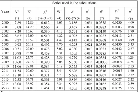
re-spective aggregates of the economy as a whole. Column 3 in Table 1 in Appendix B reports
the estimates for this ratio. They relate to the business sector of the U.S private economy over
the said period, whereas the sources of the data and certain conventions adopted in the
calcu-lations are described in the notes section at the bottom of the table.
Estimates of the minimum building labor of producers’ goods may be obtained by starting from the expression:
ˆ ( )
( ) ( ) , 0, ,14
ˆ ( )
wK t
k t k t t
wK t
. (28′)
Employing (1), (5) and (26), this can be re-written as:
7
( ) ( )
( ) , 0, ,14
ˆ ( )
p t K t
k t t
wL t
. (28″)
Implicit in (28″) is that the time it takes to construct each unit of producers’ goods is zero. To relax this assumption, but also for computational purposes, it helps to introduce two
adjust-ments. The first is to write (28) in the following modified form:
( ) ( )
( ) , 0, ,14
ˆ ( )
p t K t
k t α t
wL t
, (28)
where α is a parameter to be computed during the solution of system (9). As for the second
ad-justment, this derives from the observation that in the model the ratio p t K t( ) ( ) /wL tˆ ( ) is the
val-ue of the undepreciated capital stock to the wage bill in the consumers’ goods industry. Hence, in line with the explanation in the preceding paragraph, an estimate of ( )k t may be obtained by
us-ing the economy wide values of the undepreciated stock of fixed assets and the wage bill at the
same level of aggregation. The estimates for this ratio are shown in Column 5 of Table 1.
Next, let us turn to the parameters. Regarding the rate of technological progressμ,
con-ventionally it is approximated by two measures: labor productivity, or output per man-hour,
and Total Factor Productivity (TFP), or output per unit of all inputs used. The former
meas-ure is more in tune with the model because it coincides with the reciprocal of the capital
co-efficient, i.e.1 / ( )b υ X υ L υ( ) / ( ). To be sure, this measure is biased in several respects. For
example, it attributes all productivity to labor, even though firms employ also producers’ goods and many other inputs in the production of goods and services; As mentioned above, it
relates exclusively to one of the sector in the economy, i.e. the consumers’ goods industry; and moreover it varies significantly from year to year, whereas technological progress,
ema-nating primarily from systematic Research and Development (R&D) efforts, is a slow moving
incremental process. To allow for these shortcomings a reasonable compromise is to adopt the
data for labor productivity as reported by the U.S. Bureau of Labor Statistics for the business
sector of the U.S. economy. But, instead of relying on the annual figures, a better choice is to
use their simple average for the years 2000-2014. Column 6 of Table 1 displays both the
an-nual figures of labor productivity as well as their simple average, giving μ-0.0209.
The figures in Column 7 give the rate of inflation as measured by the Consumer Price Index
(CPI). Each figure in this series constitutes an approximation to the target rate of inflation that
the central bank had set in the particular year. While solving equation (26) it would be more
not converge, particularly because of the negative inflation rate in the year 2009. For this reason
the series of inflation was approximated by its mean, i.e. by setting θ0.0238
Columns 8 and 9 display two series ofg. In the model this was defined as the growth rate of
the labor force. Doing so was appropriate because it set the minimum rate of growth that the
economy ought to achieve for attaining and maintaining full employment stable equilibrium
economic growth. But if technological change and/or other reasons enable the economy to
achieve higher rates of economic growth, the appropriate rates to use would be those higher
rates. On this basis, in the computationsgis approximated by the figures in column 8 that
rep-resent the growth rates of the U.S. economy.
Finally, some details about the parameters , and α η ρ. In the computations their values are
determined iteratively so as to achieve convergence in the solution of system (9). In
particu-lar, during the solution the Solve algorithm in the mathematical software package Mathcad
was directed to assign such values to them so as to maximize pairwise the correlation between
the computed series ( ( ), ( ))u tc i tˆc and the reported series ( ( ), ( ))u tr i tr from official U.S.
gov-ernment and semi-govgov-ernment sources.
3.2 Comparative analysis of computed and reported series of key variables
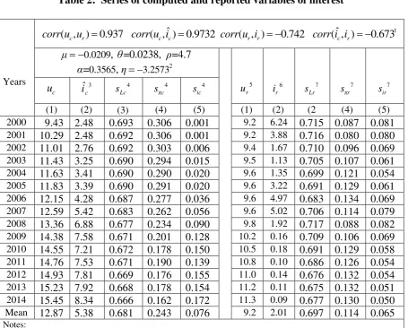
Table 2 in Appendix B consists of two sections. The one on the left presents the main series
of interest that were computed from the model, whereas the one on the right displays the same
series that were retrieved from the sources mentioned in the notes section of the table. The
figures in the top two rows give the values of the parameters for which the computed series
hold, as well as the correlations among certain selected pairs of computed and reported series.
Looking closer at this table, several key results stand out. To facilitate their presentation
and interpretation, Figure 1 brings together the computed and the reported series in a uniform
visual setting. In particular, in order to add the time perspective in the discussion, the reported
series have been extended as far back as the 1950s. From the graphs of ( ) and ( )u tc u tr we
ob-serve that: (a) both series are increasing; (b) the difference of u tc( ) over u tr( ) grows larger
by the year, and (c) given from Table 2 that they are correlated to the tune of 0.937, the series
( ) c
u t tracks the series u tr( ) extremely well. These findings ascertain with comfortable
mar-gins of confidence that the stock of producers’ goods in the U.S private economy is getting older from the early years of the 1980s, and indeed since 2000 at much faster rates than those
estimated by the national income and product accountants. Hence, unless it is propagated by
high-ly unlikehigh-ly,8 this persistent upward trend of the average useful life of producers’ goods should be due to other reasons that need to be identified and explained, because the aging of the capital
stock in an economy is intimately related to the slowdown in productivity, the deceleration in
economic growth, the decline in the labor share, etc.
Certainly, there may be many reasons that have shaped this trend. The parameters in the
second row from the top in Table 2 reveal that the model accounts for three of them. These
are technological change, shifts in the competitive structure of markets, and monetary policy.
Regarding technological change, the value of μ embedded in the calculations may be biased
upwards, if not from a long term perspective, at least since 2005. Therefore, given that ceteris
paribusμ is related negatively with ( )u t , the true upward trend in the series u tc( )may be a bit
sharper. Turning to the market structure, recall that the value of η results from the solution of
system (9) that maximizes the correlation between the series ( ) and ( )u tc u tr . This implies
that it is derived endogenously and that it cannot be assessed empirically whether it is
reason-able or not. However, it should be noted that ceteris paribus the higher is the output price elas-ticity of demand, and hence the more competitive are the markets for consumers’ goods, the
8
lower the useful lives of producers’ goods that are employed. Lastly, the model accounts for changes in monetary policy that are channeled through the numeraire and the nominal interest
rate. According to Buiter (2007), decoupling of the numeraire from the other functions of
money is still far from being adopted as an instrument of monetary policy. Hence, the value of
0.112
ρθ may stand for the rate of increase in the quantity of money capital. Of this rate
0.0209 percentage points might be aimed at monetizing technological change, because then
0.0209 0
μ , whereas the rest might aim at achieving other objectives, including the target
rate of inflation θ0.0238.
In the model all effects from expanding the quantity of money capital are channeled to the
equilibrium useful life of producers’ goodsu tc( ) through changes in the nominal equilibrium
rate of interest ( )i tˆc , which in turn bring about changes in the real equilibrium rate of interest
( ) c
i t .9 Exactly as we would expect from capital theory and past experience in mature market
economies, Figure 1 shows that these two variables are related positively and strongly, and
more precisely from Table 2 to the extent of 0.973. By contrast, as we see in Figure 1, the
federal funds rate ( )i tr moves opposite to the nominal and real equilibrium interest rates,
giv-ing for the period since 2000 a correlation of -0.742 (see top row of Table 2).10 Moreover,
ob-serve in Figure 1 that in the decades going back to 1950s the federal funds rate moved
oppo-site to the reported useful life of producers’ goods, thus rendering it most likely that the feder-al funds rate moved opposite to the equilibrium interest rate throughout the post war period.
These findings are highly puzzling, and hence, in need of an explanation.
One that comes to mind is the following. Suppose that the U.S. economy sometime in the
early years of the 1980s switched from a capital abundant to a capital scarce phase. From
cap-ital theory and past experience we would expect firms to switch to policies for economizing in
the use of fixed assets by slowing down or even postponing plans for new expansionary and
re-placement investments. As a result the useful life of the stock of producers’ goods would change course and from declining it would turn increasing. This shift is consistent with the path
in Figure 1 of the reported useful lives u tr( ) since 1950, as well as with the computed useful
livesu tc( )since 2000. But while the switching from relative abundance to relative scarcity of
investable resources in the real economy is reflected in the rising of the useful lives of
9
Mishkin (1996) reviews the channels of monetary policy and emphasizes the importance of changes in the real interest rate for monetary policy to be effective.
10
ers’ goods, in the money capital market it surfaces as a rising interest rate. Why then have the U.S. monetary authorities been driving the federal funds rates opposite to these fundamentals?
A possible answer is that they lean against the wind in the sense that they try to play a balancing
act by sending signals opposite to the ones that prevail in the economy just to discourage the
creating of bubbles due to animal spirits and other excesses. However, doing so is not without
welfare costs, because in the process they may distort, for example, the distribution of income in
unknown magnitudes and directions. Whether this possibility in the form of testable hypotheses
is confirmed or refuted by the data is an issue that will be taken up in the next section.
Columns 3, 4 and 5 in Table 2 give the income shares of labor, profits and interest. The
ones shown in the left section are percentages of income allocations derived from the model.
Hence they are based on the net value added in the business sector of the U.S private
econo-my. Those shown in the right section are similar percentages reckoned on the basis of gross
domestic income in the particular manner explained in note 6 of the table. On inspection, it
can be seen that the share of profits from the model is much higher than that derived from the
U S. National Income and Product me Accounts (NIPA), of the U.S Bureau of Economic
Analysis (BEA). The reason is that the model allocates to profits sources of incomes that BEA
accounts separately, because they cannot be allocated with certainty among labor, profits and
interest. However, this difficulty presents no problem for our purposes, because the only
as-pect that matters here is the trends reflected in these series and not their levels. On this basis,
Figure 2 displays the three pairs of income shares in order to identify and draw attention to
important differences in the ways they have evolved since 2000.
The graphs at the top relate to the computed and the reported series of the labor share. We
observe that both decline, the former somewhat slower and with much less variability than the
latter. Actually the rates at which they decline per annum are so small that this evidence may
be viewed as a confirmation of the result from equation (23) that the labor share is free of
any time trend. In turn these findings lead to the near certainty that the decline in the labor
share is due mainly to the forces that have been allowed for in the model and that whatever
differences in the variability between the computed and the reported series of the labor
share are due to unaccounted forces like the changes in monetary policy that are channeled
to the real economy through the federal funds rate.
Significant are also the findings regarding the shares of profits and interest. In the period
under consideration these evolved as shown by the graphs in the lower part of Figure 2. The
pair of graphs colored brown depicts the series of computed and reported share of profits,
observe is that the computed share of profits and interest move opposite to those reported.
The difference, particularly with regard to the share of profits, is important not because it
con-trasts sharply with the established wisdom, which sides with the view that the share of profits
is increasing, but because if the equilibrium share of profits is indeed on a downward trend,
several puzzling questions about the deceleration of investment and productivity can be
ex-plained by appeal to rational entrepreneurial decisions. As for the rising equilibrium share of
interest, the explanation is straightforward. The net stock of producers’ goods on which inter-est income is reckoned grows faster because: first, as the useful life of producers’ goods i n-creases the net stock of such goods declines slower, and, second, as the depreciation of the producers’ goods in place declines the proportion of expansionary investment in gross in-vestment grows. Thus, given that at the same time the equilibrium interest rate rises, the share
of interest increases. Expressed in another way, the share on non-labor income increases,
al-beit mildly, not because the profits share is increasing but because of the increasing interest share due to the increasing average useful life of producers’ goods and the increasing nom i-nal, and hence real, equilibrium interest rate.
Finally, in order to get a glimpse into the differences in the levels, the variability and the
rates of decline in the reported and the computed share of labor, Table 3 in Appendix B brings
together the series sLc and sLr from Table 2 with two additional series sLr and sLr
from the
three reported series indicate that the labor share has been declining and that the series
comput-ed from the model is consistent with this finding. So there is no doubt about this stylizcomput-ed fact. But
otherwise the differences in their levels and variability are wide, with the largest observed
be-tween the series from BEA and BLS. As a matter of fact, given that the latter series includes some allocation from the share of proprietors’ incomes, whereas the series from BEA is comprises only the compensation of employees, the difference between the two series is even wider.
3.3 Market structure and the share of labor
By virtue of condition (11) the firms in the model are endowed with some monopoly power in
their markets and they can set the prices of their products so as to maximize the unit net worth
of the producers’ durables they employ. This monopoly power is associated with a finite price elasticity of demand that translates into profits over and above what the firms pay out in the
form of interest to money capital owners. From Table 2 it can be ascertained that in the 15
year period under consideration with a price elasticity of aggregate demand for consumer
goods equal to -2.865, the computed average share of profits was 21.6 percent.
Instead, let us abandon for the moment the above conceptualization and concentrate on the
case in which all markets in the economy are perfectly competitive. Since this implies that the
1 1
η η
. (11′)
The value of the expression / (1η η) would decline from 1.536 in the model to 1; the labor
share according to expression (23) would increase as much as required to drive the share of
profits to zero; and the net national income would be allocated only in the form of labor
in-comes and interest payments. Consequently, by drawing on these implications in comparison
to the results from the model, we may surmise that: (a) the degree of monopoly power firms
command and exercise in the economy is intimately related to the level of labor share; (b)
changes in the monopoly power of firms affect the share of labor in the opposite direction; (c)
public policies which intentionally or unintentionally increase (decrease) the monopoly power
of firms should be expected to decrease (increase) the share of labor, and (d) monetary policy,
in particular, may affect the labor share both directly through its influence on the interest rate
and indirectly by encouraging or discouraging the concentration of firms among others
through the process of mergers and acquisitions. That is why keen competition, first and
foremost in the money capital markets, is of primary importance and interest.
However, gauging the monopoly power of firms and especially in the economy as a whole
faces many difficulties. Some are conceptual. For example, if a concentration index shows
that a small number of firms realize a very large percentage of the overall sales in the
econo-my, this by itself does not imply necessarily that the firms use their market power to set
abu-sively high prices, since their profits may come from innovative activities or efficiency gains
that eventually may benefit the consumers. Some other difficulties emanate from the nature
of the available data. The case in this regard is that the data which can be accessed, say from
the cite http://www.census.gov/epcd/www/concentration.html, are reported for five year
peri-ods and refer to manufacturing, not the overall economy. Lastly, by most indications
concen-tration in the aggregate economy appears to be decreasing rather than increasing. For instance,
according to the U.S. Economic Census in 1997 the fifty largest U.S. companies accounted
for 24 percent of the value added in manufacturing. This percentage was the same in 1992 and
even in 1954, whereas by such measures as the percentage of total employment and total
as-sets controlled by the 50, 100, or 200 largest firms, industrial concentration in the U S.
actu-ally has declined since World War II.
From the above it follows that concentration in the U.S. economy is unlikely
to have increased the monopoly power of firms, at least not to an extent that it
2000. This narrows whatever adverse effects may have been exerted from this source to
pos-sible concentration gains in the banking sector, particularly due to mergers, acquisitions and
liquidations of failed banks during the 2007-10 economic turmoil. The following excerpt from
Wheelock (2011, 167) draws on considerable evidence showing that concentration in this
sec-tor has not increased:
“…this article finds that except for a few rural banking markets, acquisitions of failed banks by in-market competitors generally had only a small impact on market concentra-tion. Most banks that failed during 2007-10 were small, and although many of those banks were acquired by much larger institutions, those acquisitions generally had little impact on market concentration. Acquisitions of larger banks that failed during 2007-10, such as the acquisition of Washington Mutual Bank by JPMorgan Chase Bank, also had only limited impact on the concentration in most of the banking markets involved. Among large MSAs, the Houston and New York City banking markets were most affect-ed by the acquisition of Washington Mutual but both remainaffect-ed relatively unconcentrataffect-ed after the acquisition.”
To conclude, the research effort below will be conducted as if the degree of concentration and
the exercise of monopoly power by U. S. firms remained stable throughout the 15 year period
under consideration.
4. Test results and interpretations
Drawing on the above findings and assessments, the emphasis in this part is on testing the
fol-lowing two hypotheses:
H1: At least since 2000 the stance of monetary policy as gauged by the federal funds rate has been easing. However, contrary to popular thinking, this policy has been perceived and acted upon by households and firms as a worsening scarcity of in-vestable resources, thus leading to a persistent rise in the equilibrium useful life of producers’ goods as well as the equilibrium nominal and real interest rates. In turn both these trends resulted in a persistent, albeit mild, decline in the share of labor. Therefore, the monetary policy may not have been as innocuous as com-monly thought with respect to this undesirable development.
H2: According to the computations, quite more sizable that the decline in the equilib-rium share of labor is the decline in the share of profits. Since during the period under consideration the degree of competition remained roughly stable, if not de-clining, it is not unlikely that the monetary policy by pushing the federal finds rates to the zero bound may have contributed to this trend.
The objective of the statistical analysis below is to confirm or refute these two hypotheses
with a comfortable margin of confidence.
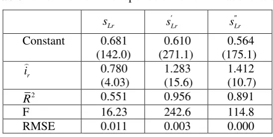
4.1 Monetary policy and the share of labor
Equation (29) presents the results from the estimation of the relationship between the