Munich Personal RePEc Archive
Forecasting with High-Dimensional Panel
VARs
Koop, Gary and Korobilis, Dimitris
University of Strathclyde, University of Essex
December 2015
Forecasting with High-Dimensional Panel VARs
∗
Gary Koop
University of Strathclyde
Dimitris Korobilis
†University of Essex
January 31, 2018
Abstract
This paper develops methods for estimating and forecasting in Bayesian panel vector autoregressions of large dimensions with time-varying parameters and stochastic volatility. We exploit a hierarchical prior that takes into account possible pooling restrictions involving both VAR coefficients and the error covariance matrix, and propose a Bayesian dynamic learning procedure that controls for various sources of model uncertainty. We tackle computational concerns by means of a simulation-free algorithm that relies on an analytical approximation of the posterior distribution. We use our methods to forecast inflation rates in the eurozone and show that forecasts from our flexible specification are superior to alternative methods for large vector autoregressions.
Keywords: Panel VAR, inflation forecasting, Bayesian, time-varying parameter
model
∗We want to thank Ana Galvao, Tony Garratt, George Kapetanios, James Mitchell, Ivan Petrella,
Rob Taylor and participants at the 9th European Central Bank Workshop on Forecasting Techniques; the Bank of England workshop on Time-Variation in Econometrics and Macroeconomics; and the 10th RCEA Bayesian Econometric Workshop, for helpful comments and discussions. All remaining errors are ours.
†Corresponding author: Essex Business School, University of Essex, Wivenhoe Park, Colchester,
1
Introduction
As the economies of the world become increasingly linked through trade and financial flows, the need for multi-country econometric modelling has increased. Panel Vector Autoregressions (PVARs), which jointly model many macroeconomic variables in many countries, are becoming a popular way of fulfilling this need. We use the general term PVAR for models where the dependent variables for all countries are modelled jointly in a single VAR and, thus, the VAR for each individual country is augmented with lagged dependent variables from other countries. In this paper, we develop econometric methods for PVARs of possibly large dimensions using a hierarchical prior which can help overcome the concerns about over-parameterization that arise in these models. The novelties of our approach are that i) we tackle in one integrated setting all concerns pertaining to out-of-sample forecasting, such as controlling for over-fitting and dealing with model uncertainty; ii) we allow for empirically relevant extensions that account for structural breaks and changing volatilities; and iii) we do so in a computationally efficient way, building on previous work by Koop and Korobilis (2013) for single-country VARs.
and Korobilis (2013), that incorporate shrinkage estimators and efficient computational algorithms. However, large VAR methods typically rely on shrinkage priors that ignore the panel structure in the data and this loss of useful information might have adverse effects in forecasting.1
Consequently, our motivation and first econometric contribution is to develop efficient methods for VARs of large dimensions that feature panel-specific restrictions as well as time-varying parameters and stochastic volatility, and fill this particular gap in the VAR literature. Our starting point is the seminal contribution of Canova and Ciccarelli (2009) who introduce a hierarchical shrinkage prior for multi-country VARs with time-varying parameters and develop Markov chain Monte Carlo (MCMC) simulation methods to tackle estimation.2 We extend their methods to account for stochastic volatility in
the panel VAR error covariance matrix. We also propose a model formulation that allows us to introduce their hierarchical shrinkage prior to the time-varying error covariance matrix. Both these extensions are empirically relevant. There is ample evidence that volatility in empirical macroeconomic models is extremely important for forecasting (see, among many others, Clark and Ravazzolo, 2015 and Diebold, Schorfheide and Shin, 2017), in which case it is imperative to relax the assumption of homoskedasticity used by Canova and Ciccarelli (2009). However, given that time-varying covariance matrices are non-parsimonious, some form of shrinkage is also needed for these parameters. Off-diagonal elements of the error covariance matrix of a panel VAR represent static/contemporaneous interdependencies among countries. This motivates our use the same pooling prior on these error covariance parameters that Canova and Ciccarelli (2009) only use for the VAR coefficients. Finally, we adapt
1
In particular, popular applications of large VARs rely on the Minnesota prior (Doan, Litterman and Sims, 1984) that places weak prior shrinkage on the intercepts and own autoregressive dynamics of each variable, but heavily shrinks cross-terms and more distant lags. In the case of panel VARs right-hand side lags include own lags of each variable of a given country, but also i) lags of the same variable of other countries; ii) lags of other variables of the same country; and iii) lags of other variables of other countries. The Minnesota prior would simply place equal prior weight on these three categories of right-hand side variables, which would result in discarding useful information about interdependencies and homogeneities among countries. Similar arguments would hold for any shrinkage prior or penalized estimator that is not developed specifically for panel VARs, such as the popular lasso of Tibshirani (1996).
2
the scalable state-space estimator of Koop and Korobilis (2013) to this time-varying parameter panel VAR setting. This estimator is simulation-free and, in combination with the pooling-shrinkage prior of Canova and Ciccarelli (2009), it allows estimation and forecasting with models with possibly hundreds of endogenous variables.
performance.
Our paper also seeks to contribute to the empirical literature on inflation modelling in the eurozone. There are many linkages and inter-relationships between the economies of the eurozone countries. Modelling aggregate inflation for the eurozone as a whole will miss many interesting country-specific patterns since monetary policy can have differing impacts on different countries. These considerations justify why we want to forecast individual country inflation rates, but not using conventional VAR methods one country at a time. The panel VAR is an effective way of modelling the spillovers and inter-linkages between countries that may exist for the eurozone countries. Euro area inflation has been an important component in many recent policy discussions. Deflation has been a recent worry. For instance, in December 2014, most of the eurozone were experiencing deflation and no country registered an inflation rate above 1%. Subsequently euro area inflation has increased, but as of 2018 it still remains low by historic standards. Although there has been a tendency for inflation rates in the various eurozone countries to converge to one another, there are still substantive cross-country differences, in particular around the time of the eurozone crisis. For instance, Delle Monache, Petrella and Venditti (2015) document the relative roles of country-specific and common shocks to euro area country inflation rates. Although commonalities predominate, country-specific shocks play a large role. Furthermore, Delle Monache, Petrella and Venditti (2015) document substantial time variation in parameters, providing additional support for our model which allows for such variation.
The remainder of the paper is organized as follows. In Section 2, we describe our econometric methods, beginning with the panel VAR before proceeding to the case of time-varying parameters and stochastic volatility, and then our dynamic treatment of model uncertainty. Section 3 contains our empirical study of euro area inflation. We find substantial evidence of forecasting benefits, in particular from using dynamic learning methods which average over different PVAR dimensions and different hierarchical priors. Section 4 concludes.
2
Econometric Methodology
and introduce the hierarchical prior we adopt, before discussing time-varying parameter versions of PVARs. We then propose modifications of the time-varying parameter PVAR model in order to allow hierarchical modelling of the error covariance matrix. We conclude this section with a discussion of our treatment of model uncertainty and provide a detailed explanation of how the dynamic learning procedure works.
2.1
Methods of Ensuring Parsimony in the PVAR
Assume N countries and G variables for each country which are observed for T time periods. In our empirical application these are 10 eurozone countries and we use inflation plus an additional eight country-specific predictor variables, observed for 216 months. Let Yt = (y1′t, y2′t, ..., y′N t) for t = 1, ..., T be the N G×1 vector of dependent variables
where y′
it is theG×1 vector of dependent variables of country i,i= 1, ..., N.3 Thei-th
equation of the PVAR with p lags takes the form
yit=A1iYt−1+...+ApiYt−p+uit, (1)
where Aji for j = 1, .., p are G × N G matrices PVAR coefficients for country i. Additionally, uit is a G×1 vector of disturbances, uncorrelated over time, where uit ∼
N(0,Σii). The errors between countries may be correlated and we defineE uitu′jt
= Σij
and Σ to be the entireN G×N Gerror covariance matrix forut = (u1t, .., uN t)′. LetAj =
Aj1, ..., AjN for j = 1, ..., p and α= vec(A1)′, ..., vec(Ap t)
′′
. Note that, for notational simplicity, we have not added an intercept or other deterministic terms nor exogenous variables, but they can be added with the obvious modifications to the formulae below. In our empirical work, we include an intercept.
The unrestricted PVAR given in (1) is likely over-parameterized, involving K =p×
(N ×G)2 unknown autoregressive parameters and N×G×(N2 ×G+1) error covariance terms. Plausible choices for N, G and p can lead to very large parameter spaces. A popular approach to dimension reduction in Bayesian vector autoregressions is to use hierarchical priors that induce shrinkage in the parameters. Examples of such priors include the scale mixture of Normals priors used in George, Sun and Ni (2008) and the priors from general equilibrium models of Del Negro and Schorfheide (2004). However, adopting any of the
3
existing priors developed for a single-country VAR will result in discarding valuable information due to the fact that one would expect partial pooling of coefficients in a panel setting. Incorporating such information could improve forecasts. Furthermore, these methods require the use of MCMC methods which make them computationally infeasible with high-dimensional models, particularly in the context of a forecasting exercise.
A popular way to introduce such pooling in PVARs that will result in efficient shrinkage, is described in Canova and Ciccarelli (2009, 2013). These authors use a certain hierarchical prior so as to work with restricted versions of (1), a practice which we adopt in this paper. In particular, we assume the following reduced rank representation of the PVAR coefficients:
α = Ξ1θ1+ Ξ2θ2+..+ Ξqθq+e
= Ξθ+e
where Ξ = (Ξ1, ..,Ξq) are known matrices and θ = θ1′, .., θq′
′
is an R ×1 vector of unknown parameters with R < K and e is uncorrelated with ut and distributed as
N(0,Σ⊗V) where V = σ2I. Due to the fact that the high-dimensional vector of
coefficientsα is projected into a lower dimensional vector of latent parametersθ, we will refer to this second layer regression as a “factor model” for the PVAR coefficients (this will become clearer later when α, θ become time-varying). This specification can be thought of as a hierarchical prior for the PVAR model of the formα|Σ∼N(Ξθ,Σ⊗V) and θ ∼N(0, Q), which is of the natural conjugate form for α due to the conditioning on Σ.
How can we use this specification to extract meaningful lower-dimensional factors of
α that take into account the panel structure in the data? Suppose, for instance, that the elements of α are made up of a common factor, a factor specific to each country and a factor specific to each variable. This is the factor structure used in Canova and Ciccarelli (2009). Then q= 3 and Ξ1 will be a K×1 vector of ones,θ1 a scalar. Ξ2 will
be a K×N matrix containing zeros and ones defined so as to pick out coefficients for each country and θ2 is anN×1 vector. Ξ3 will be a K×Gmatrix containing zeros and
For instance, if N =G= 2 and p= 1 then
Ξ2 =
ι1 0
ι1 0
0 ι2
0 ι2
and Ξ3 =
ι3 0
0 ι4
ι3 0
0 ι4
where ι1 = (1,1,0,0)′, ι2 = (0,0,1,1)′, ι3 = (1,0,1,0)′ and ι4 = (0,1,0,1)′. Thus, the
K dimensional αis dependent on a much lower dimensional vector of parameters, since
θ is of dimension R = 1 +N +G with e being left to model any residual variation in the parameters. Such a strategy can be used to greatly reduce the dimensionality of α
and help achieve parsimony. However, such a method may come at a cost if the factor structure is not chosen correctly. The latter could lead either to over-parameterization concerns or to mis-specification concerns. In the previous example, where the coefficients are assumed to depend on a common factor, a country specific factor and a variable specific factor, it could be, e.g., that no common factor exists (θ1 = 0) and a specification
which ignored this restriction would over-parameterized. On the other hand, our example of a factor structure might be too restrictive and mis-specification might result. The
K distinct elements of α may be so heterogeneous that a factor structure with only
N +G+ 1 parameters may not be adequate.
These considerations suggest that the model space should be augmented using different choices of Ξ and an algorithm developed to choose between them. This is what we do in this paper. In theory, one could devise a huge range of possible structures for Ξ, e.g. allowing own lag coefficients to be unrestricted; impose “core” and “periphery” clusters on the coefficients; global VAR restrictions, and so on. In practice, we have found that for our euro area data two specific structures clearly beat a range of several other options in terms of in-sample and out-of-sample fit. The first is one begins with the same pooling structure proposed in Canova and Ciccarelli (2009) but leaves intercepts and first autoregressive lagged coefficients to be unrestricted – meaning that these sets of coefficients are not determined through the common factors. This can simply be achieved if we extract one factor for each coefficient we want to leave unrestricted and set the state variance of that parameter to zero. If, as an example, the j-th element of
has it’sj-th scalar element equal to one, and all remainingK−1 elements equal to zero. That way, we add 2×N ×G factors to the ones that already Canova and Ciccarelli suggest.4
The second way of specifying the factor structure is by restricting Ξ in such a way that the PVAR collapses to a country-specific VAR structure. To explain what we mean by this, let p = 1 and consider the N G2 coefficients in the VAR for country i. G2
of these coefficients are on lags of country i variables, with the remaining (N −1)G2
being on lags of other countries’ variables. We define Ξ such that its accompanying θ
loads only on the G2 coefficients that are on lags of country ivariables. Thus, if e= 0,
the coefficients on other country variables are zero and the PVAR breaks down into
N individual VARs, one for each country (apart from any inter-linkages which occur through Σ). The impacts of other countries’ variables on country i are only allowed for through the presence of e. Intuitively, this structure for Ξ captures the idea that working with VARs one country at a time comes close to being adequate (i.e. most of the coefficients on lagged country j variables in the country i VAR will be zero), but there are occasional inter-linkages which can be captured through e. When we move to the time-varying parameter PVAR (TVP-PVAR) in the next section, this definition of Ξ will imply the same intuition, except in terms of individual-country TVP-VARs.
2.2
Moving from the PVAR to the TVP-PVAR
We begin by putting t subscripts on all the PVAR coefficients in (1) and, thus, αt =
vec(A1
t)
′
, ..., vec(Apt)
′′
is the K×1 vector collecting all PVAR parameters at time t. We write the TVP-PVAR in matrix form as:
Yt =Xt′αt+ut, (2)
where Xt = I ⊗ Yt′−1, ..., Yt′−p
′
, and ut ∼ N(0,Σt). An unrestricted time-varying
parameter VAR would typically assume αt to evolve as a random walk (see, e.g., Doan,
Litterman and Sims, 1984, Cogley and Sargent, 2005, or Primiceri, 2005). However, in
4
the multi-country TVP-PVAR case this may lead to an extremely over-parameterized model and burdensome (or even infeasible) computation. At each point in time t the number of PVAR parameters, p×(N×G)2, could run into the thousands or more. The fact that in the case of time-variation we haveT such high-dimensional parameter vectors only complicate computations. Adding to the mix the fact that typical estimation would rely on MCMC methods (e.g. Cogley and Sargent, 2005, use MCMC), means that we have to repeat thousands of times any burdensome algorithmic operations involving these high-dimensional parameter vectors. Repeatedly running such an algorithm on an expanding window of data, as is typically done in a recursive forecasting exercise, multiplies this burden by hundreds in many applications. As discussed in Koop or Korobilis (2013), estimating TVP-VARs using MCMC methods can easily become computationally infeasible unless the number of forecasting models and their dimension are both small.
In order to achieve parsimony, we follow Canova and Ciccarelli (2009) and extend the factorization of the PVAR coefficients described in the preceding subsection to the time-varying case using the following hierarchical prior:
αt = Ξθt+et (3)
θt = θt−1+wt, (4)
where θt is an R × 1 vector of unknown parameters, R ≪ K, Ξ is defined as
in the preceding subsection and wt ∼ N(0, Wt) where Wt is an R × R covariance
matrix, and extending Canova and Ciccarelli (2009)’s homoskedastic specification we let
et ∼N(0,Σt⊗V) where V = σ2I. The factors θt evolve according to a random walk,
in order to be consistent with the bulk of the time-varying parameter VAR literature we cited above. The hierarchical representation of the panel VAR using equations (2), (3) and (4) resembles the hierarchical time-varying parameter SUR specified in Chib and Greenberg (1995). However, the generic MCMC sampler of Chib and Greenberg (1995), when applied to the hierarchical prior above, proves to be computationally inefficient. This is because their algorithm requires many draws from the Normal conditional posterior of αt ∀t, which proves to be extremely demanding. In this case, a certain
assumption that the prior forαtin equation (3) is of natural conjugate form (conditional
on Σt) comes in handy.
As a consequence, we can simplify the TVP-PVAR given by (2), (3) and (4) into the following simpler, two-equation form (see Canova and Ciccarelli, 2013, page 22, for a proof):
Yt = Xet′θt+vt, (5)
θt = θt−1+wt, (6)
where Xet =XtΞ and vt = Xt′et+ut with vt ∼ N(0,(I+σ2Xt′Xt)×Σt). Therefore, in
this form the TVP-PVAR is written as a Normal linear state-space model consisting of the measurement equation in (5) and the state equation (6). For known values of Σt,
Wt and σ2, standard methods for state space models based on the Kalman filter can be
used to obtain the predictive density and posterior distribution for θt.Thus, we will not
repeat the relevant formulae here and the reader is referred to the Technical Appendix of this paper, as well as Koop and Korobilis (2013) for further computational details. A typical Bayesian analysis would involve using MCMC methods to draw Σt, Wt and σ2
and then, conditional on these draws, use such state space methods. However, in our case, the computational burden of MCMC methods will be prohibitive. Accordingly, we use: i) forgetting factor methods to provide an estimate of Wt, ii) Exponentially
Weighted Moving Average (EWMA) methods to estimate Σt and, iii) use a grid of
values for σ2 and interpret each value as defining a particular model and, thus, include
them in our model space when we take model uncertainty into account (see the next subsection). The following paragraphs elaborate on these points.
First, in any state-space problem estimation of the state variance (Wt in our case)
means that Wt can be estimated using the following formula
c
Wt =
1
λ −1
var(θt|Dt−1),
whereDt−1 denotes data available through periodt−1, 0< λ≤1 is the forgetting factor
(typically set to a value lower than one but close to it) and var(θt|Dt−1) is a predicted
variance readily available at time t from the Kalman filter iteration of the previous time period, t−1. Thus, at the cost of using a method which is approximate, we gain huge benefits in terms of computational simplicity and stability.5 The forgetting factor
approach allows estimation of systems with large numbers of variables in seconds, and, hence, is computationally attractive for recursive point and density forecasting or any other state space modelling exercise that can become infeasible using MCMC methods. Improving on the inference of Canova and Ciccarelli (2009), we allow for the TVP-PVAR error covariance matrix to be time-varying and use EWMA filtering methods to estimate it as:
b
Σt =κΣbt−1+ (1−κ)eutue′t,
where ueteu′t = (I+σ2Xt′Xt)
−1
Yt−Xet′E(θt|Dt−1) Yt−Xet′E(θt|Dt−1)
′
,
E(θt|Dt−1) is produced by the Kalman filter and 0 < κ ≤ 1. κ is referred to as a
decay factor. We define the κ = 1 case to be Σbt =
Pt
τ=1ueτeu′τ
t (i.e. equivalent to least
squares methods in a homoskedastic model). In order to initializeΣbt, we setΣb0 = 0.1×I
which is a relatively diffuse choice.
The forgetting factor λ and decay factor κ control the amount of time variation in the system. Lower (higher) values of λ, κ imply faster (slower) changes over time in the values of θt and Σt, respectively. When λ = κ = 1 then both θt
and Σt become time invariant and we have the constant parameter homoskedastic
PVAR. In our empirical work, we let λ = {0.990,0.992,0.994,0.996,0.998,1.000} and κ = {0.92,0.94,0.96,0.98,1.00}, interpret each grid point as defining a model and use dynamic model selection methods (to be described below) to select the optimal value. Thus, the data can select either the constant coefficient PVAR or
5
Likelihood-based methods, such as Bayesian and maximum likelihood inference, rely on formulae involving var(θt|Dt). However, at time t this quantity is uknown and needs to be estimated reliably,
homoskedastic PVAR at any point in time, or can select a greater degree of variation in coefficients or error covariance matrix. We adopt a similar strategy for σ2, using a grid
of σ2 ∈ {0.001,0.003,0.005,0.007,0.009, 0.01,0.03,0.05,0.07,0.09, 0.1,0.3,0.5,0.7,0.9,
1,3,5,7,9}.
The Kalman filter provides us with a one-step ahead predictive density. Since we wish to forecast at horizon h >1 and calculate predictive likelihoods, we use predictive simulation for longer forecast horizons. To do this, we draw YT+1 from its Normal
predictive density with mean and variance given by the Kalman filter (these are assumed to be constant and fixed during predictive simulation), then simulate YT+2 from its
Normal predictive density conditional on the drawn YT+1, etc. up to h.
2.3
A Hierarchical Prior for the Error Covariance Matrix
As we have seen, the error covariance matrix of the TVP-PVAR can also be huge, leading to a desire for shrinkage on it as well. In this subsection, we extend the hierarchical prior of Canova and Ciccarelli (2009) to allow for such shrinkage. We decompose the error covariance matrix as Σt =Bt−1Ht HtBt−1
′
where Bt is a lower triangular matrix with
ones on the diagonal, Ht is a diagonal matrix and write the VAR as
Yt=Xt′αt+Bt−1Htεt,
where εt∼N(0, I). We can write the model in the following form as:
Yt =Xt′αt+Wt′βt+Htεt, (7)
where Wt is the matrix
Wt=
0 . . . 0
ε1t 0 . . . 0
0 [ε1t, ε2t] . .. ...
... . .. . .. 0 0 . . . 0 ε1t, ..., ε(N G−1)t
With this specification we have an equivalent model where the error covariances show up as contemporaneous regressors on the right hand side of the TVP-PVAR. This model cannot be estimated as a multivariate system using standard filtering methods described previously. To see this, note that elements Yt show up both on the left-hand side, and
the right-hand side of the PVAR (via the matrix of contemporaneous error terms, Wt).
In this case, the state-space system is nonlinear and multivariate estimation would need to rely on computationally intensive simulation methods. A potential solution to this problem would be to follow Carriero, Clark and Marcellino (2016) and estimate the model equation-by-equation: the first equation does not contain any contemporaneous information on the right-hand side so can be estimated independently of other equations using a linear filter; the second equation is dependent on ε1t which can be replaced by
residuals from the first equation; the third equation is dependent onε1t, ε2twhich can also
be replaced by residuals, and so on until equation N G which also depends on residuals available from the previous N G−1 equations.6 However, such an option is not available
to us, since the pooling prior we adopt clusters coefficients among different equations. As a consequence the parameters of different PVAR equations will not be independent a-posteriori, and equation-by-equation estimation is not available. We overcome this issue in a fashion similar to the problem of estimating time-varying covariance matrices using the EWMA specification described in the previous subsection. That is, when constructingWtwe replaceεt with the one-step ahead residuals from each Kalman filter
iteration, namely εet =Yt−Xt′E(αt|Dt−1)−Wt′E(βt|Dt−1). Doing so allows each time
period t to have all right-hand-side variables observed and proceed with the estimation methods described in the previous section.
In order to complete this new but equivalent PVAR specification that treats elements
6
In a previous version of this manuscript we were instead working with the model
Yt=Xt′γt+Zt′βt+Htεt,
whereγt=
vec BtA 1 t
′
, ..., vec(BtA p t)
′′
andZthad the same structure asWtbut with elements−Yjt
in place ofεbjt – see also the definition of the respective matrixZtin the Appendix of Primiceri (2005).
This previous formulation of the VAR and the one we currently use in equation (7) are observationally equivalent, however, the latter offers the advantage of having the original VAR coefficientαtremaining
the vector of VAR coefficients as in our original specification in (2). In contrast, the VAR form described above is in terms of coefficients γt which consist of products of VAR coefficients At and the VAR
covarianceBt. In this case, applying the pooling prior onγtinstead of the original VAR coefficientsαt
of the error covariance matrix as exogenous predictors, we can extend our previous approach and introduce a hierarchical prior on both αt and βt of the form:
δt ≡
"
αt
βt
# =
"
Ξα 0
0 Ξβ
#
θt+ut≡Ξθt+ut, (8)
θt = θt−1+vt.
where now ut ∼ N(0, HtHt⊗(σ2I)), which has a diagonal covariance matrix since
both Ht and σ2I are diagonal matrices. Under the additional assumption that Ξ is
block diagonal and αt and βt load on separate factors (rows of θt), then we have prior
independence between the two sets of coefficients. This exact prior independence of the sets of coefficients – an assumption that is used extensively in many Bayesian applications (see Primiceri, 2005) – is a crucial assumption that allows for equation-by-equation estimation of the PVAR using the linear Kalman filter. The econometric methods described in the preceding subsection can be used directly, with a slight simplification due to the diagonality of Ht.
The two choices for Ξα are those described at the end of Section 2.1. For Ξβ we
also use these two choices with the trivial adaptation required by the structure for
Wt. In the forecasting exercise we allow for Ξα and Ξβ to potentially be different.
Using P (for pooled) subscripts to denote the form that builds on Canova and Ciccarelli (2009), and CS (for country-specific) subscripts to denote the country-specific VAR factor structure, we define four possible specification for the Ξ matrices: i) Ξα
P and Ξ β P,
ii) Ξα
P and Ξ β
CS, iii) Ξ α
CS and Ξ β
P and iv) Ξ α
CS and Ξ β
CS. As we explain next in the
following subsection, selection of the best specification pair for Ξα and Ξβ is part of a
more general dynamic procedure that selects the values of various hyperparameters that are optimal for forecasting.
2.4
Dynamic Treatment of Model Uncertainty
The previous subsections discussed the estimation of single time-varying parameter PVARs and defined our model space. Our most general approach involves a model space where the models differ in various features, in order to explicitly control for model uncertainty. The features defining the models include the different choices for λ, κ and
sub-section 2.3; and different PVAR dimensions (to be described in sub-section 3.1). In total we have 16,800 PVAR or TVP-VAR models to choose between. In this sub-section, we describe how to do so in a dynamic manner such that the chosen model may change over time. Our methods use posterior model probabilities constructed in a dynamic manner.
We can use such posterior model probabilities to either do model selection or averaging. In this paper, we adopt the view that some of our specification choices relate to concepts which can be interpreted as parameters (i.e. λ, κ and σ2). For these we do
model selection since this is similar to estimating them (e.g. if we select a model with
λ= 0.99 this is the same as estimatingλto be 0.99). We also do model selection for the different choices for Ξα and Ξβ since they define different priors and presenting results
which average over very different priors would reduce the interpretability of results. With regards to choosing the dimension of the PVAR, this is more like a conventional modelling choice. For this, we use model averaging methods following standard Bayesian practice. Of course, the econometric methods developed in this paper could be used to use a single approach throughout (e.g., do only dynamic model selection over all models in our model space).
To be precise, for Ξα, Ξβ, λ,κ and σ2, we choose the values that maximize posterior
model probabilities. Conditional on the optimal choice of these, we then estimate TVP-PVARs with different numbers of endogenous variables and provide forecasts which average over them. That is, we produce forecasts from every model and then our final forecast is a weighted average of them, where the weights are given by their respective posterior model probabilities.
Calculating posterior model probabilities can also be computationally burdensome, especially with a vast array of models. In addition, most conventional methods are not dynamic (e.g. simply calculating the marginal likelihood for each model). In the remainder of this sub-section, we outline a computationally simple method for the calculation of posterior model probabilities in a dynamic fashion, comparable with the Kalman filter update rules used for parameter estimation (i.e. we predict time t model probabilities given information at time t−1, and then update these probabilities when time t information becomes observed).
Let M(i) for i = 1, ..., J be the set of models under consideration, which in our
about the optimal configuration for forecasting we need to quantify a measure of belief for each single model. We follow Raftery et al (2010) and do so by calculating dynamic model probabilities, p M(i)|D
t−1
, for each model. We use forgetting factor methods to estimate p M(i)|D
t−1
. The forgetting factor literature (e.g. Kulhav´y and Kraus, 1996 and Raftery, Karny and Ettler, 2010) provides derivations and additional motivation for how sensible estimates forp M(i)|D
t−1
can be produced in a fast, recursive manner, in the spirit of the Kalman filtering approach. Here we outline the basic steps, following the exponential forgetting factor approach of Kulhav´y and Kraus (1996). Let ωt(|it)−1 =
p M(i)|D
t−1
be the probability associated with model i for forecasting Yt using data
available through timet−1. The general version of the algorithm combines a prediction step
ωt(|it)−1 =
ωt(−i)1|t−1µ
PJ j=1
ωt(−j)1|t−1µ
, (9)
with an updating step
ωt(|it) ∝ωt(|it)−1p Yt|M(i),Dt−1
, (10)
with a normalizing constant to ensure the ω(t|it) sum to one. p Yt|M(i),Dt−1
is the predictive density produced by the Kalman filter, evaluated at the realized value forYt.
The recursions begin with an initial condition for the weights, which we set at ω(0i|)0 = J1 (i.e. all models have equal prior probability).
The quantity 0 < µ ≤ 1 is a forgetting factor used to discount exponentially more distant observations in a similar fashion to λ. Since p Yt|M(i),Dt−1
is a measure of forecast performance, it can be seen that this approach attaches more weight to models which have forecast well in the recent past. To see this clearly, note that (9) can be written as
ω(t|it)−1 ∝
t−1
Y
i=1
p Yt|M(i),Dt−1
µi .
With monthly data and µ= 0.99, this equation implies that forecast performance one year ago receives about 90% as much weight as forecast performance last period, two years ago receives about 80% as much weight, etc. This is the value used by Raftery, Karny and Ettler (2010) and in our empirical work.
our models differ in Yt (i.e. they have a different number of endogenous variables). To
surmount this problem, p Yt|M(i),Dt−1
is replaced by p YC
t |M(i),Dt−1
where YC t is
the set of variables which are common to all models. In our application, these are the three variables which are included in our smallest TVP-PVAR (see sub-section 3.1) for every country. We refer to the approach as the TVP-PVAR with a dynamic learning prior: TVP-PVAR (DLP). We use this terminology since the prior is hierarchical and dynamic so we can learn about which panel structure is appropriate to impose on the coefficients. Finally, note that it is also possible to include lag length selection as another specification choice and do dynamic model selection over p in a time-varying fashion. However, we do not do so to keep the computational burden manageable. Canova and Ciccarelli (2009) set p = 1 for all their specifications involving TVP-PVARs. Allowing for p > 1 is possible and we found that p = 2 provides optimal inflation forecasts compared to other choices. Hence, our empirical results use p= 2.
3
Forecasting Euro Area Inflation
3.1
Data
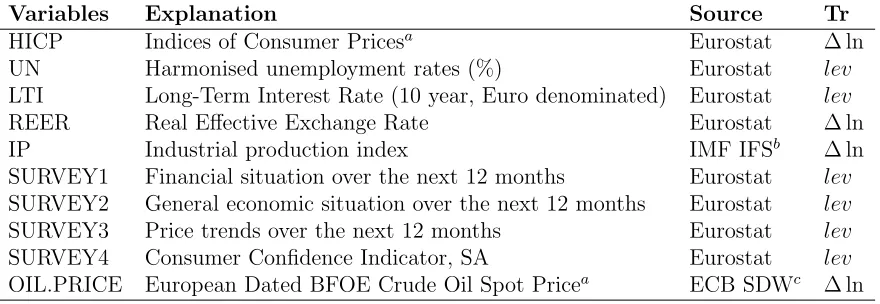
Variables Explanation Source Tr
HICP Indices of Consumer Pricesa Eurostat ∆ ln
UN Harmonised unemployment rates (%) Eurostat lev
LTI Long-Term Interest Rate (10 year, Euro denominated) Eurostat lev
REER Real Effective Exchange Rate Eurostat ∆ ln
IP Industrial production index IMF IFSb ∆ ln
SURVEY1 Financial situation over the next 12 months Eurostat lev
SURVEY2 General economic situation over the next 12 months Eurostat lev
SURVEY3 Price trends over the next 12 months Eurostat lev
SURVEY4 Consumer Confidence Indicator, SA Eurostat lev
OIL.PRICE European Dated BFOE Crude Oil Spot Pricea ECB SDWc ∆ ln
a
Variables that are not seasonally adjusted by the provider, are adjusted by the authors using the X11 filter in Eviews.
b
International Monetary Fund, International Financial Statistics
c
European Central Bank, Statistical Data Warehouse
3.2
Estimation Using the TVP-PVAR with Dynamic Learning
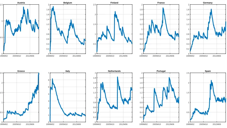
[image:20.612.88.528.97.249.2]Before comparing the forecasting performance of TVP-PVAR (DLP) to some popular alternatives, it is useful to see which specification choices are receiving the most weight in our model averaging exercise.
Figure 1 plots the volatilities in the inflation equations for all countries using TVP-PVAR (DLP) methods. We emphasize that our algorithm allows for the optimal choice of the degree of time variation in parameters through the choice of κ. The algorithm could have chosen κ = 1 (homoskedasticity), but based on visual inspection of Figure 1, it clearly is not doing so. Figure 1 shows a high degree of heteroskedasticity in all countries. Note, too, that the patterns of volatility vary substantially across countries.
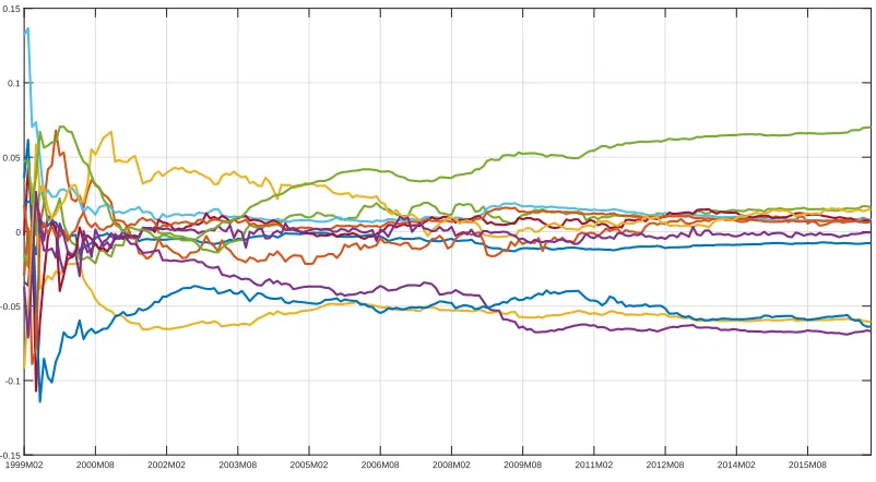
Figure 1 relates to the error variances. Does the substantial heterogeneity and fluctuation in volatility we are finding for them also occur with the time-varying covariances? We are finding that it does not. To illustrate this point, remember that our specification in equation (7) leads to the error covariances being in βt which are
then pooled using common factors as in (8). Due to the high-dimensionality of βt,
1999M020 2005M10 2012M06 0.5
1
1.5 Austria
1999M020 2005M10 2012M06 0.2 0.4 0.6 0.8 1 1.2 1.4 1.6 1.8 2 Belgium
1999M020 2005M10 2012M06 0.5
1 1.5 2
2.5 Finland
1999M020 2005M10 2012M06 0.2 0.4 0.6 0.8 1 1.2 1.4 1.6 1.8 2 France
1999M020 2005M10 2012M06 0.2 0.4 0.6 0.8 1 1.2 1.4 1.6 1.8 2 Germany
1999M02 2005M10 2012M06 0 0.5 1 1.5 2 2.5 Greece
1999M02 2005M10 2012M06 0 1 2 3 4 5 6 7 Italy
1999M02 2005M10 2012M06 0 0.2 0.4 0.6 0.8 1 1.2 1.4 1.6 1.8 2 Netherlands
1999M02 2005M10 2012M06 0 0.2 0.4 0.6 0.8 1 1.2 1.4 1.6 1.8 2 Portugal
[image:21.612.113.509.98.321.2]1999M02 2005M10 2012M06 0 0.5 1 1.5 2 2.5 Spain
Figure 1: Point estimates of error variances in inflation equations
is substantially less fluctuation of these covariance factors over time7. Note that we do
not plot the factors relating to time-varying VAR coefficients αt in equation (7) due to
the fact that they are so numerous.
7
1999M02 2000M08 2002M02 2003M08 2005M02 2006M08 2008M02 2009M08 2011M02 2012M08 2014M02 2015M08 -0.15
[image:22.612.108.509.102.323.2]-0.1 -0.05 0 0.05 0.1 0.15
Figure 2: Posterior mean estimates of covariance matrix common factors implied by the pooling prior.
2005M12 2007M06 2008M12 2010M06 2011M12 2013M06 2014M12 2016M06 0
0.1 0.2 0.3 0.4 0.5 0.6 0.7 0.8 0.9
1 Time-varying probabilities of selection of different Ξ matrices
ΞP α
and ΞP β
ΞP α and ΞCS
β
ΞCS α
and ΞP β
ΞCS α and ΞCS
[image:23.612.111.509.99.322.2]β
Figure 3: Posterior mean probabilities attached to different choices for Ξ
2005M120 2007M06 2008M12 2010M06 2011M12 2013M06 2014M12 2016M06 0.1
0.2 0.3 0.4 0.5 0.6 0.7 0.8 0.9 1
3 variables per country (30-variable VAR) 4 variables per country (40-variable VAR) ...
[image:24.612.110.509.102.324.2]9 variables per country (90-variable VAR)
Figure 4: Posterior mean probabilities attached to different choices for G
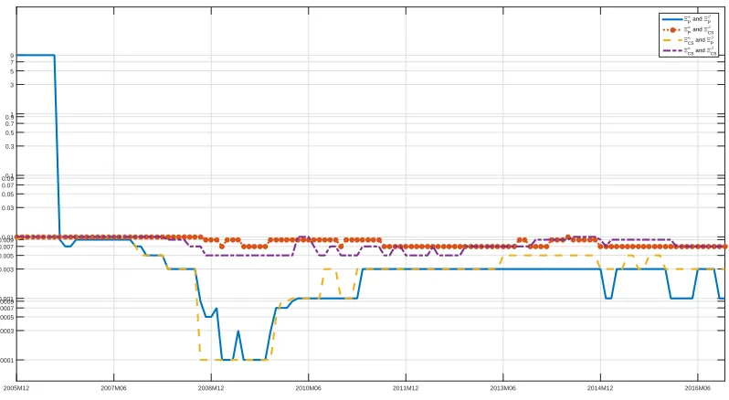
Figure 5 relates to the scale parameter σ2 and plots the optimal value selected at
each point in time for the four different possible configurations of Ξα,Ξβ matrices in
that state equation. Note that the vertical axis is in the logarithmic scale, which allows us to plot in a single graph all possible values of σ2 specified in our grid. Here again we
can see some time variation in the optimal choice for this parameter. There is also a fair degree of sensitivity to the structure of Ξ. When we use Canova and Ciccarelli (2009)’s choice of Ξ, then the optimal value of σ2 is lower than when using the country-specific
factor structure, particularly between 2008 and 2010. This pattern in our data-base estimates of σ2 is roughly consistent with the choice of Canova and Ciccarelli (2009)
who in their empirical work set for simplicity σ2 = 0. However, when we use
country-specific restrictions σ2 tends to be different from zero. It is clearly worth estimating this
2005M12 2007M06 2008M12 2010M06 2011M12 2013M06 2014M12 2016M06 0.0001
0.0003 0.0005 0.0007 0.0009 0.001 0.003 0.005 0.007 0.009 0.01 0.03 0.05 0.07 0.09 0.1 0.3 0.5 0.7 0.9 1 3 5 7 9
ΞP
α
and ΞP
β ΞP
α and ΞCS
β ΞCS
α
and ΞP
β ΞCS
α and ΞCS
[image:25.612.110.509.102.321.2]β
Figure 5: Optimal values for σ2 selected by DMS for different choices for Ξ
In this subsection, we have presented evidence that TVP-PVAR (DLP) captures important patterns in the data in a manner that a single model could not. But, ultimately, the test of our approach lies in forecasting and it is to this we now turn.
3.3
Forecasting using TVP-PVAR (DLP)
3.3.1 Models for Comparison
following paragraphs and provide complete specification details of all approaches in the Technical Appendix.
First, relative to other approaches for high-dimensional VARs, our dynamic learning prior allows for the model to learn which panel prior is appropriate. This motivates a comparison with other Big Data approaches which do not allow for this sort of learning. Thus, we include a conventional large Minnesota prior VAR similar to the popular specification of Ba´nbura, Giannone and Reichlin (2010) but with optimal degree of shrinkage estimated as in Giannone, Lenza and Primiceri (2015). We also include a dynamic factor model and a factor augmented VAR. We abbreviate these three approaches as BVAR, DFM and FAVAR, respectively.
Second, relative to other large VAR approaches which do incorporate a panel structure in the hierarchical prior, our approach allows for time-variation in parameters. This motivates comparison with a model with a panel structure similar to our own, but without time-variation in the parameters. We consider a version of the constant parameter model of Canova and Ciccarelli (2009) which is nested within our TVP-PVAR (DLP) approach. This uses their choices of Ξα
P and Ξ β
P and setsλ=κ= 1, thus
ensuring a homoskedastic model with no time-variation in PVAR coefficients. We do not do model averaging over VAR dimensions with this approach. All other specification and modelling choices (including treatment of σ2) is the same as in our TVP-PVAR
(DLP) approach. This is labelled PVAR (CC09) in the tables.
Third, our TVP-PVAR (DLP) considers two different panel structures in the hierarchical prior. However, several other structures have been proposed in the literature. An influential one allows for the investigation of whether there are dynamic or static interdependencies between countries as described in Canova and Ciccarelli (2013). We consider a hierarchical prior which allows for the selection or omission of these types of interdependencies between countries. We adopt the approach of our earlier work, Koop and Korobilis (2016), which develops a simulation algorithm called stochastic search specification selection (SSSS) to find such interdependencies if they exist and refer to the approach as PVAR (SSSS). We also consider a restricted version of our approach which leads to a single TVP-PVAR of the form considered in Canova and Ciccarelli (2009). That is, we use the full set of endogenous variables, select Ξα
P and Ξ β
P as done in
and Ciccarelli (2009). Our use of forgetting factor methods (as opposed to MCMC) mean estimation and forecasting are computationally feasible.
Fourth, our approach differs from many approaches that estimate a model for each country individually. As a representative of this class of models, we present forecasts from country specific VARs and abbreviate this approach as CS-VAR. We also consider two popular univariate models which we run one country at a time. These are the unobserved components stochastic volatility (UCSV) model of Stock and Watson (2007) and an extension of the UCSV model which allows for AR lags with time varying coefficients on the right hand side. The latter model, which we label TVP-AR, was found by Pettenuzzo and Timmermann (2017) to provide good forecasts of inflation.
Finally, in Big Data models there is a growing interest in use of machine learning methods. Such methods are starting to work their way into the VAR literature and it is of interest to compare our approach to something from this emerging literature. The general idea of this literature is to allow an algorithm to automatically search through the myriad possible specification choices without much input from the economist. This contrasts with conventional approaches used in econometrics where the researcher carefully designs a hierarchical prior based on empirical insight into the problem at hand (e.g. the factor structure Σα
P reflects the empirical wisdom expressed in Canova
and Ciccarelli, 2009, as to how VARs in different countries might be related to one another). In Koop, Korobilis and Pettenuzzo (2017), we developed a particular type of machine learning algorithm using random compression methods for large VARs. In the present paper, we forecast with it and refer to it as BCVAR. See the Technical Appendix or Koop, Korobilis and Pettenuzzo (2017) for exact details on how this method works, but the key point to stress here is that it does not reflect the multi-country nature of our data set. Rather each equation in the VAR receives an identical treatment and it is left to the algorithm to uncover the nature of any inter-linkages across countries.
Complete details of these models are given in the Technical Appendix.
coefficients (by choosing λ= 1) or the error covariance (by choosing κ= 1), but it does not. Our approach could have chosen smaller PVARs (by choosing G= 3), but it does not always do so. Thus, comparison with these types of restrictions on our models is less interesting than comparison with other plausible non-nested alternatives which are described above.
3.3.2 Forecasting Results
We evaluate statistically forecasts of inflation from the models introduced in the previous sub-section relative to a benchmark approach which produces forecasts using individual AR(2) models for each country’s inflation series. We forecastpt+h−ptwhereptis the log
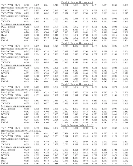
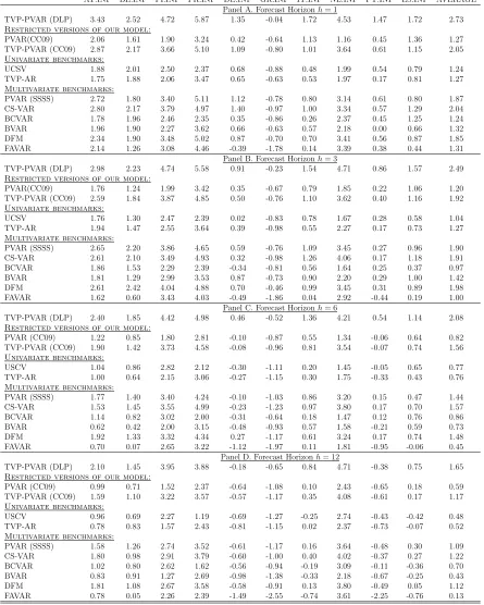
of a country’s prices at time t for various forecast horizons. Our forecasts are produced recursively on an expanding window of data. We present Mean Squared Forecast Errors (MSFEs) and Averages of Log Predictive Likelihood (ALPLs) in order to evaluate point and density forecasts, respectively. In the tables in this sub-section, we present results for the 10 inflation rates in the 10 countries in our sample as well as an average across all countries. For the MSFEs, we use a simple average (and divide by the comparable figure using the AR(2) benchmarks). For the ALPLs, the cross-country average is based on the multivariate predictive density for the 10 inflation series and the comparable figure from the AR(2) benchmark is subtracted off. The forecast evaluation period is 2006M1-2016M12.
It can be seen that, when we look at cross-country averages, our TVP-PVAR (DLP) approach is forecasting best particularly at short horizons. This holds true regardless of whether we use MSFEs or ALPLs as measures of forecast performance. We elaborate on these points in the remainder of this section in relation to the five features mentioned at the beginning of the preceding sub-section.
Incorporating the panel structure in the prior in a dynamic fashion is helping improve forecast performance. A comparison of the TVP-PVAR (DLP) results to a conventional Minnesota prior large VAR indicates the former is forecasting better at all horizons, regardless of whether MSFE or ALPL is used as a forecast metric. The same holds for the DFM and FAVAR approaches.
(CC09)) we find, without exception, evidence in favour of the TVP-PVAR (DLP). This holds true regardless of whether MSFEs or ALPLs are used as a measure of forecast performance. This suggests that it is not enough to allow for selection of different panel priors in the context of a constant coefficient models, one must do so in a dynamic fashion allowing for the panel structure to change.
Next we compare the forecast performance of our approach to the alternative panel structure in the prior of PVAR (SSSS). Recall that this latter algorithm was proposed by Koop and Korobilis (2016) in order to stochastically search for all combinations of static and dynamic interdependencies that can possibly occur among N countries. However, being a computationally expensive simulation-based approach, this approach only features constant coefficients and covariance. As a consequence, this alternative is also consistently beaten by our current approach in terms of forecast performance. Similarly PVAR (CC09) which uses the single factor structure of Canova and Ciccarelli (2009) in a constant coefficient model provides forecasts inferior to our approach. Even allowing for time-variation in parameters (but constant volatilities) as in the TVP-PVAR (CC09) does not substantially improve things.
Working with individual country models such as CS-VAR, UCSV or TVP-AR also produces, on average, consistently worse forecast performance over all forecast horizons and both forecast metrics. Finally, the TVP-PVAR (DLP) is even forecasting better than the approach inspired by the machine learning literature: BCVAR.
Table 1. MSFEs relative to AR(2) for the period 2006M1-2016M12
AT.INF BE.INF FI.INF FR.INF DE.INF GR.INF IT.INF NL.INF PT.INF ES.INF AVERAGE Panel A. Forecast Horizonh= 1
TVP-PVAR (DLP) 0.620 0.785 0.651 0.719 0.881 0.964 0.676 0.854 0.970 0.869 0.799
Restricted versions of our model:
PVAR(CC09) 0.752 0.891 0.707 0.949 0.890 1.014 0.773 0.931 1.005 1.021 0.893
TVP-PVAR (CC09) 0.729 0.873 0.692 0.926 0.871 0.990 0.759 0.915 0.983 1.011 0.875
Univariate benchmarks:
UCSV 0.661 0.854 0.721 0.759 0.882 0.888 0.786 0.867 1.034 0.904 0.836
TVP-AR 0.653 0.845 0.711 0.750 0.879 0.880 0.775 0.861 1.036 0.901 0.829
Multivariate benchmarks:
PVAR (SSSS) 0.782 0.808 0.788 0.758 0.840 0.987 0.747 0.851 1.047 1.093 0.870
CS-VAR 0.675 0.812 0.806 0.766 1.080 1.015 0.715 1.042 1.046 0.918 0.887
BCVAR 0.706 0.894 0.708 0.815 0.960 0.992 0.861 1.004 1.148 1.004 0.909
BVAR 0.716 0.877 0.700 0.917 0.882 0.987 0.763 0.906 0.974 1.015 0.874
DFM 0.720 0.933 0.679 1.022 0.822 0.902 0.859 0.821 1.027 0.948 0.873
FAVAR 0.701 0.892 0.741 0.786 0.913 0.912 0.829 0.896 1.066 0.937 0.867
Panel B. Forecast Horizonh= 3
TVP-PVAR (DLP) 0.647 0.795 0.663 0.873 0.825 1.072 0.849 0.885 1.012 1.025 0.865
Restricted versions of our model:
PVAR(CC09) 0.745 0.892 0.732 0.945 0.932 0.927 0.796 0.913 1.028 1.126 0.904
TVP-PVAR (CC09) 0.733 0.884 0.716 0.928 0.917 0.913 0.790 0.907 1.009 1.109 0.891
Univariate benchmarks:
UCSV 0.694 0.806 0.687 0.889 0.856 1.148 0.901 0.931 1.075 0.974 0.896
TVP-AR 0.686 0.794 0.683 0.888 0.855 1.147 0.891 0.930 1.072 0.972 0.892
Multivariate benchmarks:
PVAR (SSSS) 0.716 0.861 0.725 0.921 0.908 1.123 0.904 0.931 1.098 1.203 0.939
CS-VAR 0.713 0.837 0.720 0.929 0.878 1.140 0.908 0.955 1.082 1.173 0.933
BCVAR 0.872 1.061 0.786 0.993 0.981 0.971 0.935 1.026 1.082 1.077 0.978
BVAR 0.737 0.877 0.727 0.926 0.922 0.930 0.795 0.907 1.006 1.096 0.892
DFM 0.712 1.127 1.017 1.142 0.906 0.934 0.868 0.764 1.123 1.215 0.981
FAVAR 0.728 0.842 0.697 0.922 0.898 1.162 0.936 0.949 1.089 1.202 0.943
Panel C. Forecast Horizonh= 6
TVP-PVAR (DLP) 0.609 0.749 0.628 0.767 0.833 0.982 0.774 0.836 1.007 1.073 0.826
Restricted versions of our model:
PVAR (CC09) 0.734 0.870 0.712 0.942 0.966 0.932 0.743 0.938 1.046 1.175 0.906
TVP-PVAR (CC09) 0.722 0.858 0.698 0.927 0.951 0.917 0.734 0.913 1.025 1.165 0.891
Univariate benchmarks:
USCV 0.675 0.813 0.686 0.881 0.869 1.084 0.831 0.880 1.055 0.953 0.873
TVP-AR 0.675 0.807 0.677 0.874 0.863 1.072 0.823 0.877 1.051 0.945 0.866
Multivariate benchmarks:
PVAR (SSSS) 0.680 0.836 0.680 0.833 0.879 1.076 0.844 0.893 1.088 1.098 0.891
CS-VAR 0.662 0.799 0.702 0.839 0.880 1.095 0.818 0.893 1.029 1.091 0.881
BCVAR 0.762 0.974 0.712 0.935 0.948 0.943 0.795 0.973 1.212 1.080 0.934
BVAR 0.711 0.866 0.690 0.939 0.954 0.934 0.730 0.920 1.031 1.168 0.894
DFM 0.744 0.963 0.704 0.878 0.699 0.931 0.729 0.661 1.082 1.014 0.841
FAVAR 0.700 0.838 0.706 0.900 0.907 1.127 0.858 0.916 1.085 1.141 0.918
Panel D. Forecast Horizonh= 12
TVP-PVAR (DLP) 0.688 0.856 0.835 0.907 0.818 0.931 0.890 0.887 1.095 1.062 0.897
Restricted versions of our model:
PVAR (CC09) 0.768 0.886 0.881 0.877 0.854 1.061 0.925 0.939 1.096 1.145 0.943
TVP-PVAR (CC09) 0.742 0.868 0.857 0.858 0.834 1.033 0.910 0.923 1.078 1.123 0.923
Univariate benchmarks:
USCV 0.644 0.769 0.722 0.862 0.781 1.109 0.929 0.940 0.976 0.941 0.867
TVP-AR 0.638 0.766 0.719 0.857 0.779 1.111 0.929 0.931 0.973 0.944 0.865
Multivariate benchmarks:
PVAR (SSSS) 0.749 0.830 0.749 0.862 0.876 1.121 0.950 0.944 1.143 1.124 0.935
CS-VAR 0.676 0.831 0.722 0.900 0.876 1.103 0.914 0.939 1.098 1.130 0.919
BCVAR 0.836 1.098 0.863 0.945 0.986 0.956 1.004 1.087 1.315 1.073 1.016
BVAR 0.677 0.821 0.757 0.853 0.847 1.038 0.914 0.923 1.080 1.130 0.904
DFM 0.695 0.851 0.810 0.922 0.896 1.252 0.973 1.055 1.083 1.281 0.982
Table 2. ALPLs relative to AR(2) for the period 2006M1-2016M12
AT.INF BE.INF FI.INF FR.INF DE.INF GR.INF IT.INF NL.INF PT.INF ES.INF AVERAGE Panel A. Forecast Horizonh= 1
TVP-PVAR (DLP) 3.43 2.52 4.72 5.87 1.35 -0.04 1.72 4.53 1.47 1.72 2.73
Restricted versions of our model:
PVAR(CC09) 2.06 1.61 1.90 3.24 0.42 -0.64 1.13 1.16 0.45 1.36 1.27
TVP-PVAR (CC09) 2.87 2.17 3.66 5.10 1.09 -0.80 1.01 3.64 0.61 1.15 2.05
Univariate benchmarks:
UCSV 1.88 2.01 2.50 2.37 0.68 -0.88 0.48 1.99 0.54 0.79 1.24
TVP-AR 1.75 1.88 2.06 3.47 0.65 -0.63 0.53 1.97 0.17 0.81 1.27
Multivariate benchmarks:
PVAR (SSSS) 2.72 1.80 3.40 5.11 1.12 -0.78 0.80 3.14 0.61 0.80 1.87
CS-VAR 2.80 2.17 3.79 4.97 1.40 -0.97 1.00 3.34 0.57 1.29 2.04
BCVAR 1.78 1.96 2.46 2.35 0.35 -0.86 0.26 2.37 0.45 1.25 1.24
BVAR 1.96 1.90 2.27 3.62 0.66 -0.63 0.57 2.18 0.00 0.66 1.32
DFM 2.34 1.90 3.48 5.02 0.87 -0.70 0.70 3.41 0.56 0.87 1.85
FAVAR 2.14 1.26 3.08 4.46 -0.39 -1.78 0.14 3.39 0.38 0.44 1.31
Panel B. Forecast Horizonh= 3
TVP-PVAR (DLP) 2.98 2.23 4.74 5.58 0.91 -0.23 1.54 4.71 0.86 1.57 2.49
Restricted versions of our model:
PVAR(CC09) 1.76 1.24 1.99 3.42 0.35 -0.67 0.79 1.85 0.22 1.06 1.20
TVP-PVAR (CC09) 2.59 1.84 3.87 4.85 0.50 -0.76 1.10 3.62 0.40 1.16 1.92
Univariate benchmarks:
UCSV 1.76 1.30 2.47 2.39 0.02 -0.83 0.78 1.67 0.28 0.58 1.04
TVP-AR 1.94 1.47 2.55 3.64 0.39 -0.98 0.55 2.27 0.17 0.73 1.27
Multivariate benchmarks:
PVAR (SSSS) 2.65 2.20 3.86 4.65 0.59 -0.76 1.09 3.45 0.27 0.96 1.90
CS-VAR 2.61 2.10 3.49 4.93 0.32 -0.98 1.26 4.06 0.17 1.18 1.91
BCVAR 1.86 1.53 2.29 2.39 -0.34 -0.81 0.56 1.64 0.25 0.37 0.97
BVAR 1.81 1.29 2.99 3.53 0.87 -0.73 0.90 2.20 0.29 1.00 1.42
DFM 2.61 2.42 4.04 4.88 0.70 -0.46 0.99 3.45 0.31 0.89 1.98
FAVAR 1.62 0.60 3.43 4.03 -0.49 -1.86 0.04 2.92 -0.44 0.19 1.00
Panel C. Forecast Horizonh= 6
TVP-PVAR (DLP) 2.40 1.85 4.42 4.98 0.46 -0.52 1.36 4.21 0.54 1.14 2.08
Restricted versions of our model:
PVAR (CC09) 1.22 0.85 1.80 2.81 -0.10 -0.87 0.55 1.34 -0.06 0.64 0.82
TVP-PVAR (CC09) 1.90 1.42 3.73 4.58 -0.08 -0.96 0.81 3.54 -0.07 0.74 1.56
Univariate benchmarks:
USCV 1.04 0.86 2.82 2.12 -0.30 -1.11 0.20 1.45 -0.05 0.65 0.77
TVP-AR 1.00 0.64 2.15 3.06 -0.27 -1.15 0.30 1.75 -0.33 0.43 0.76
Multivariate benchmarks:
PVAR (SSSS) 1.77 1.40 3.40 4.24 -0.10 -1.03 0.86 3.20 0.15 0.47 1.44
CS-VAR 1.53 1.45 3.55 4.99 -0.23 -1.23 0.97 3.80 0.17 0.70 1.57
BCVAR 1.14 0.82 3.02 2.00 -0.31 -0.64 0.18 1.47 0.12 0.76 0.86
BVAR 0.62 0.42 2.00 3.15 -0.48 -0.93 0.57 1.58 -0.21 0.59 0.73
DFM 1.92 1.33 3.32 4.34 0.27 -1.17 0.61 3.24 0.17 0.74 1.48
FAVAR 0.70 0.07 2.65 3.22 -1.12 -1.97 0.11 1.81 -0.95 -0.06 0.45
Panel D. Forecast Horizonh= 12
TVP-PVAR (DLP) 2.10 1.45 3.95 3.88 -0.18 -0.65 0.84 4.71 -0.38 0.75 1.65
Restricted versions of our model:
PVAR (CC09) 0.99 0.71 1.52 2.37 -0.64 -1.08 0.10 2.43 -0.65 0.18 0.59
TVP-PVAR (CC09) 1.59 1.10 3.22 3.57 -0.57 -1.17 0.35 4.08 -0.61 0.17 1.17
Univariate benchmarks:
USCV 0.96 0.69 2.27 1.19 -0.69 -1.27 -0.25 2.74 -0.43 -0.42 0.48
TVP-AR 0.78 0.83 1.57 2.43 -0.81 -1.15 0.02 2.37 -0.73 -0.07 0.52
Multivariate benchmarks:
PVAR (SSSS) 1.58 1.26 2.74 3.52 -0.61 -1.17 0.16 3.64 -0.48 0.30 1.09
CS-VAR 1.80 0.98 2.91 3.79 -0.60 -1.00 0.40 4.02 -0.37 0.27 1.22
BCVAR 1.02 0.80 2.62 1.62 -0.56 -0.94 -0.19 3.09 -0.11 -0.36 0.70
BVAR 0.83 0.91 1.27 2.69 -0.98 -1.38 -0.33 2.18 -0.67 -0.25 0.43
DFM 1.81 1.08 2.67 3.58 -0.58 -0.91 0.13 3.80 -0.49 0.05 1.12
4
Conclusions
References
[1] Ba´nbura, M., Giannone, D., and Reichlin, L. (2010), “Large Bayesian Vector Autoregressions,”Journal of Applied Econometrics, 25, 71-92.
[2] Bauwens, L., Koop, G., Korobilis, D., and Rombouts, J. (2015). “The Contribution of Structural Break Models to Forecasting Macroeconomic Series,”Journal of Applied Econometrics, 30, 596-620.
[3] Bernanke, B. S., Boivin, J., and Eliasz, P. (2005). “Measureing the Effects of Monetary Policy: A Factor-Augmented Vector Autoregressive (FAVAR) Approach,”Quarterly Journal of Economics, 120, 387-422.
[4] Canova, F. (1993), “Modelling and Forecasting Exchange Rates using a Bayesian Time Varying Coefficient Model,” Journal of Economic Dynamics and Control, 17, 233-262.
[5] Canova, F., and Ciccarelli, M. (2009), “Estimating Multicountry VAR Models,”International Economic Review, 50, 929-959.
[6] Canova, F., and Ciccarelli, M. (2013), “Panel Vector Autoregressive models: A Survey,”Advances in Econometrics, 32, 205-246.
[7] Chib, S. and Greenberg, E. (1995), “Hierarchical Analysis of SUR models with Extensions to Correlated Serial Errors and Time-varying Parameter Models,”Journal of Econometrics, 68, 339-360.
[8] Chudik, A. and Pesaran, H. (2011), “Infinite-Dimensional VARs and Factor Models,”Journal of Econometrics, 163, 4-22.
[9] Clark, T. E. and Ravazzolo, F. (2015), “Macroeconomic Forecasting Performance under Alternative Specifications of Time-Varying Volatility ”Journal of Applied Econometrics, 30, 551-575.
[11] Dees, S., di Mauro, F., Pesaran, M.H., and Smith, V. (2007), “Exploring the International Linkages of the Euro Area: A Global VAR analysis,”Journal of Applied Econometrics, 22, 1-38.
[12] Del Negro, M. and Schorfheide, F. (2004), “Priors from General Equilibrium Models for VARs,”International Economic Review, 45, 643-673.
[13] Delle Monache, D., Petrella, I. and Venditti, F. (2015), “Common Faith or Parting of Ways? A Time-varying Parameter Factor Analysis of Euro Area Inflation,”Advances in Econometrics, forthcoming.
[14] Diebold, F. X., Schorfheide, F. and Shin, M. (2017), “Real-Time Forecast Evaluation of DSGE Models with Stochastic Volatility,”Journal of Econometrics, 201, 322-332.
[15] Doan, T., Litterman, R., and Sims, C. (1984), “Forecasting and Conditional Projection Using Realistic Prior Distributions,”Econometric Reviews, 3, 1-100.
[16] Faust, J. and Wright, J. (2013), “Forecasting Inflation,” chapter 1 in Handbook of Economic Forecasting, volume 2A, G. Elliot and A. Timmermann, eds., Amsterdam: North Holland.
[17] Feldkircher, M. and Huber, F. (2016), “The International Transmission of US shocks – Evidence from Bayesian Global Vector Autoregressions,”European Economic Review, 81, 167-188.
[18] Giannone, D., Lenza M. and Primiceri, G. (2015), “Prior Selection for Vector Autoregressions,”Review of Economics and Statistics, 97, 436-451.
[19] George, E. I., Sun, D. and Ni, S. (2008), “Bayesian Stochastic Search for VAR Model Restrictions,”Journal of Econometrics, 142, 553-580.
[20] Harvey, D., Leybourne, S. and Newbold, P. (1997), “Testing the Equality of Prediction Mean Squared Errors,”International Journal of Forecasting, 13, 281-291.
[22] Koop, G., (2014), “Forecasting with Dimension Switching VARs,”International Journal of Forecasting, 30, 280-290.
[23] Koop, G. and Korobilis, D., (2013), “Large Time-varying Parameter VARs,”Journal of Econometrics, 177, 185-198.
[24] Koop, G. and Korobilis, D. (2016), “Model Uncertainty in Panel Vector Autoregressive Models,”European Economic Review, 81, 115-131.
[25] Koop, G., Korobilis, D. and Pettenuzzo, D. (2018), “Bayesian Compressed Vector Autoregressions,”Journal of Econometrics, forthcoming.
[26] Korobilis, D. (2016), “Prior Selection for Panel Vector Autoregressions,”Computational Statistics and Data Analysis, 101, 110-120.
[27] Kose, M. A., Otrok, C., and Whiteman, C. (2003), “International Business Cycles: World, Region, and Country-Specific Factors,”American Economic Review, 93, 1216-1239.
[28] Kulhav´y, R., and Kraus, F. (1996), “On Duality of Regularized Exponential and Linear Forgetting,”Automatica, 32, 1403-1415.
[29] L¨utkephol, H. (2005) New Introduction to Multiple Time Series Analysis. Heidelberg: Springer Berlin.
[30] Pettenuzzo, D., and Timmermann, A. (2017), “Forecasting Macroeconomic Variables Under Model Instability,” Journal of Business and Economic Statistics, 35, 183-201
[31] Primiceri, G. (2005), “Time Varying Structural Vector Autoregressions and Monetary Policy,”Review of Economic Studies, 72, 821-852.
[32] Raftery, A., Karny, M., and Ettler, P. (2010), “Online Prediction Under Model Uncertainty via Dynamic Model Averaging: Application to a Cold Rolling Mill,”Technometrics, 52, 52-66.
[34] Stock, J. and Watson, M. (2007). “Why has U.S. Inflation Become Harder to Forecast?” Journal of Money, Credit and Banking,39, 3-33.
A
Technical Appendix
A.1
Writing the PVAR in triangular form
Before discussing Kalman filter estimation of the model, we briefly prove a standard result in VARs and general systems of equations, that says that under a certain Cholesky ordering, the likelihood of multivariate systems can be written as a collection of independent equations. The time-varying parameter PVAR with stochastic volatility is of the form8
Yt=AtYt−1+ut, (11)
where ut ∼N(0,Σt). We allow the Cholesky-like decomposition Σt =Bt−1Ht HtB−t1
′
where Bt−1 is the unitriangular matrix
Bt−1 =
1 0 ... 0
β(2,1)t 1 . .. ...
... . .. . .. 0
β(N G,1)t ... β(N G,N G−1)t 1
, (12)
and Ht is a diagonal matrix of standard deviations. In this case we can solve the PVAR
as
Yt = AtYt−1+ut, (13)
= AtYt−1+Bt−1εt, (14)
where εt ∼ N(0, Ht). Given the triangular structure of B−t1 described above, we can
write thei-th equation of the PVAR (assuming now thati doesn’t index only countries, rather all N G variables in the model) using the following form
Yit =αitYi,t−1+β(2,1)tε1t+....+β(i,i−1)tε(i−1)t+εit. (15)
8
For notational simplicity we illustrate the PVAR(1) without intercept, but our results can obviously be generalized when the RHS is not just Yt−1 but a more general matrix of the form
Zt = (1, Yt−1, Yt−2, ..., Yt−p, dt) where dt might include dummies, exogenous and other deterministic
Using this form it is now more clear how the contemporaneous coefficients β(·)t enter
in this form as RHS predictors. This formulation converts the likelihood function into a collection of N G univariate likelihoods, where the coefficients across equations are independent (while coefficients within equations might be correlated). However, for our estimation purposes this is not true as the pooling prior of Canova and Ciccarelli (2009) clusters together coefficients from different equations. Therefore, even if the likelihood is independent accross equations, this is not true for the prior which makes equation-by-equation inference impossible. In order to deal with this issue, we replace
ε1t to ε(i−1)t with their predicted values from the Kalman filter at iteration t, i.e.
ε1(t|t−1), ..., ε(i−1)(t|t−1), ...,. In this case, we can write the PVAR in the equivalent SUR
form we presented in the text, that is
Yt =Xt′αt+Wt′βt+εt, (16)
where Xt =IN G⊗Yt−1, Wt is the matrix
Wt =
0 . . . 0
ε1(t|t−1) 0 . . . 0
0 [ε1t, ε2t] . .. ...
... . .. . .. 0
0 . . . 0 ε1(t|t−1), ..., ε((N G−1)(t|t−1))t
,
and αt=vec(At),βt= β(2,1)t, ...., β(N G,N G−1)t
.
A.2
State-space estimation
Given our desire to extend Canova and Ciccarelli (2009) and allow a time-varying covariance matrix Σt and apply the pooling prior on that covariance matrix we have
The full model we can now estimate is of the form
Yt = Xt′αt+Wt′βt+εt, (17)
"
αt
βt
# =
"
Ξα 0
0 Ξβ
#
θt+ut, (18)
θt = θt−1+vt.
We can write more compactly as
Yt = G′tδtεt, (19)
δt = Ξθt+ut, (20)
θt = θt−1+vt,
whereGt= [Xt, Wt],δt = [αt, βt] and Ξ =
Ξα,Ξβ. Recall also that nowε
t∼N(0, Ht).
The novelty of the Canova and Ciccarelli (2009) approach is to write this hierarchical state-space model that involves one measurement and two state equations into an equivalent, regular form incorporating one measurement and one state equation. As demonstrated in the text, and proven in Canova and Ciccarelli (2009), this equivalent form is
Yt = Ge′tθtǫt, (21)
θt = θt−1+vt, (22)
where ǫt ∼ N(0,(I +σ2G′tGt)×Ht). It is this final state-space form that can be
estimated trivially using the Kalman filter algorithm of Koop and Korobilis (2013) and the reader is referred to this paper for more details. The only difference is that in the transformed model Ht is a diagonal matrix so its elements will follow a collection of
univariate exponentially weighted moving average (EWMA) models, compared to the case of Koop and Korobilis (2013) who deal with a measurement (VAR) covariance matrix that is non-diagonal and which evolves as a multivariate EWMA model.
given knowledge of Ξ, we can reconstruct the parameters in the original PVAR model in (11). Even when doing predictive simulation in order to calculate predictive likelihoods – a procedure that involves sampling by simulation the future path of θt for periods
t+ 1, ..., t+h – we can still follow a “backward” procedure for recoveringAt+1, ..., At+h.
Once we have the parameters of the simple PVAR form, we can forecast using standard formulas for VARs; see L¨utkephol (2005).
B
Competing models
B.1
Unobserved Component Stochastic Volatility
The Stock and Watson (2007) unobserved components stochastic volatility (UC-SV) model is a univariate specification that only allows for a time-varying intercept, that is, it is a local level specification of the form
Yit = τit+εit, (23)
τit = τit−1+ηit, (24)
for inflation of country i in our dataset. The novelty with this specification is that both the measurement error εit and the variance of state error ηit feature stochastic volatility
specifications (hence the full models comprises two more equations describing random walk evolution of these two volatility parameters). This model has been specifically proposed for forecasting inflation 9, but it is a possibly parsimonious and flexible
nonlinear specification that can fit other series as well. We fit this model with fairly standard priors that are as diffuse as possible – considering that this is a model where the intercept varies as a random walk and completely diffuse (noninformative) priors, that would only allow the likelihood to fully determine parameter estimates, are not possible. The reader is referred to Bauwens, Koop, Korobilis and Rombouts (2015) for the exact settings used in this model.
9
B.2
Time-varying parameter autoregression
The time-varying parameter autoregression extends the UC-SV model by allowing autoregressive dynamics, that is, it is of the form
Yit = βitxit+εit, (25)
βit = βit−1+ηit, (26)
where now xit = (1, Yit−1, Yit−2)′ includes both a time-va