Using Semantics for Granularities of Tokenization

of Tokenization

Martin Riedl

martin.riedl@ims.uni-stuttgart.de

Chris Biemann

University of Hamburg Language Technology Group

biemann@informatik.uni-hamburg.de

Depending on downstream applications, it is advisable to extend the notion of tokenization from low-level character-based token boundary detection to identification of meaningful and useful language units. This entails both identifying units composed of several single words that form a multiword expression (MWE), as well as splitting single-word compounds into their meaningful parts. In this article, we introduce unsupervised and knowledge-free methods for these two tasks. The main novelty of our research is based on the fact that methods are primarily based on distributional similarity, of which we use two flavors: a sparse count-based and a dense neural-count-based distributional semantic model. First, we introduce DRUID, which is a method for detecting MWEs. The evaluation on MWE-annotated data sets in two languages and newly extracted evaluation data sets for 32 languages shows thatDRUIDcompares favorably over previous methods not utilizing distributional information. Second, we present SECOS, an algorithm for decompounding close compounds. In an evaluation of four dedicated decompounding data sets across four languages and on data sets extracted from Wiktionary for 14 languages, we demonstrate the superiority of our approach over unsupervised baselines, sometimes even matching the performance of previous language-specific and supervised methods. In a final experiment, we show how both decompounding and MWE information can be used in information retrieval. Here, we obtain the best results when combining word information with MWEs and the compound parts in a bag-of-words retrieval set-up. Overall, our methodology paves the way to automatic detection of lexical units beyond standard tokenization techniques without language-specific preprocessing steps such as POS tagging.

Submission received: 5 July 2017; revised version received: 10 February 2018; accepted for publication: 15 May 2018.

1. Introduction

If we take Ron Kaplan’s motivation for tokenization seriously that the “stream of characters in a natural language text must be broken up into distinct meaningful units” (Kaplan 2005) to enable natural language processing beyond the character level, then tokenization is more than the low-level preprocessing task of treating interpunctua-tion, hyphenainterpunctua-tion, and enclitics. Rather, tokenization also should aspire to produce meaningfulunits, or, as Webster and Kit (1992) define it, tokens should be linguistically significant and methodologically useful. In practice, however, tokenizers are rather not concerned with meaning or significance—placed right at the beginning of any NLP pipeline and usually implemented in a rule-based fashion, they are merely workhorses to enable higher levels of processing, which includes a reasonable split of the input into word tokens and some normalization to cater to the sensitivity of subsequent processing components. Although it is clear that the methodological utility of a specific tokenization depends on the overall task, it seems much more practical to fix the tokenization in the beginning of the text ingestion process and handle task-specific adjustments later. The work presented in this article operationalizes lexical semantics in order to identify meaningful units. Assuming that low-level processing has already been performed, we devise a method that can identify multiword units, namely, word n-grams that have a non-compositional meaning, as well as a method that can split close compound words into their parts. Both methods are primarily based on distributional semantics (Harris 1951): By operationalizing language unit similarity in various ways, we are able to inform the tokenization process with semantic information, enabling us to yield meaningful units, which are shown to be linguistically valid and methodologically useful in a series of suitable evaluations. Both methods do not make use of language-specific processing, thus could be applied directly after low-level tokenization without assuming the existence of, for example, a part of speech tagger.

Depending on the task, the low-level “standard” tokenization can be too fine-grained, as from a semiotic perspective multiword expressions (MWEs) refer to a single concept. On the flipside, tokenization can be too coarse-grained, as close compound words are detected as single words, whereas they are formed by the concatenation of at least two stems and can be considered as MWEs without white spaces. In this article, we will describe two different approaches to represent (nominal) concepts in a similar fashion. This results in an extended tokenization, similar to the work by Hassler and Fliedl (2006). However, they extend their tokenization solely by bracketing phrases and MWEs and do not split text in more fine-grained units. Trim (2013) differentiates between low-level and high-level tokenization. Whereas high-level tokenization con-centrates on the identification of MWEs and phrases, low-level tokenization mostly splits words that are connected by apostrophes or hyphens. Our notion of coarse-grained tokenization is similar to high-level tokenization. However, the fine-coarse-grained tokenization goes one step beyond low-level tokenization, as we split close compound words.

As a second contribution, we present a method for splitting close compounds. Examples for such close compounds include, for example, dishcloth (English), pancake (English), Hefeweizen (German for wheat beer), bijenzwerm (Dutch for swarm of bees) or hiilikuitu (Finnish for carbon fibre). Similar to MWEs, compounds are created by combining existing words, although in close compounds the stems are not separated by white space. Detecting the single stems, calleddecompounding, showed impact in several natural language processing (NLP) applications like automatic speech recog-nitions (Adda-Decker and Adda 2000), machine translation (Koehn and Knight 2003), or information retrieval (IR) (Monz and de Rijke 2001) and is perceived as a crucial component for the processing of languages that are productive with respect to this phenomenon.

For both the detection of MWEs and the decompounding of words, most existing approaches rely either on supervised methods or use language-dependent part-of-speech (POS) information. In this work, we present two knowledge-free and unsuper-vised (and therefore language-independent) methods that rely on information gained by distributional semantic models that are computed using large unannotated corpora, namely, word2vec (Mikolov et al. 2013) and JoBimText (Biemann and Riedl 2013). First, we describe these methods and highlight how their information can help for both tok-enization tasks. Then, we present results for the identification of MWEs and afterwards show the performance of the method for decompounding. For both tasks, we first show the performance using manually annotated gold data before we present evaluations for multiple languages using automatically extracted data sets from Wikipedia and Wik-tionary. Lastly, we demonstrate how both flavors of such an extended tokenization can be used in an IR setting. The article is partly based on previous work (Riedl and Biemann 2015, 2016) that has been substantially extended by adding experiments for several languages and showing the advantage of combining the methods in an information retrieval evaluation.

The article is organized as follows. Section 2 describes the distributional semantic models that are used to compute similarities between lexical units, which are the main source of information for both fine- and coarse-grained tokenization. Then, we describe how multiword expressions can be detected and evaluate our methodology. In Section 4, we describe the workings and the evaluation for compound splitting. How to use both methods for information retrieval is shown in Section 5. In Section 6, we present the related work. Afterwards, we highlight the main findings in the conclusion in Section 7 and give an overview of future work in Section 8.

2. Using Distributional Semantics for Fine- and Coarse-Grained Tokenization

Such information is beneficial when it comes to the task of splitting compounds, as we shall see subsequently. When computing similarities not only for words but considering word n-grams, we observe that concepts that are composed of several word units are often similar to single-word terms. For example, the word hot dog is most similar to food-related terms likehamburgerorsandwich. As shown in the remainder of this article, the information of distributional semantics is beneficial for the tasks of identifying of MWEs but also for the task of compound splitting.

In this work, we compute semantic similarities using the dense vector-based CBOW model from word2vec (Mikolov et al. 2013) and a symbolic graph-based approach called JoBimText (Biemann and Riedl 2013). In order to use both models within the word splitting and the word merging task, we transform them to a so-called distributional thesaurus (DT) as defined by Lin (1997). A DT can be considered as a dictionary where for each word the topnmost similar words are listed, ordered by their similarity score. The CBOW model is learned during the task of predicting a word by its context words. For this, the input layer is defined by the contexts of a word. As output layer we use the center word. The prediction is performed using a single hidden layer that represents the semantic model with the specified dimensions. For the computation of word2vec models, we use 500 dimensions, 5 negative samples, and a word window of 5. Because the implementation by Mikolov et al. (2013)1does not support the computation of similarities between alln-grams within a corpus, we use the word2vecf implemen-tation by Levy and Goldberg (2014).2This implementation allows specifying terms and contexts directly and features the functionality to retrieve the most relevant contexts for a word. In order to extract a DT from models computed with word2vec and word2vecf, we compute the cosine similarity between all terms and extract, for each term, the 200 most similar terms.

As opposed to the mainstream of using dense vector representations, the approach by Biemann and Riedl (2013), called JoBimText, uses a sparse count-based context representation that nevertheless scales to arbitrary amounts of data (Riedl and Biemann 2013). Furthermore, this approach has achieved competitive results to dense vector space models like CBOW and SKIP-gram (Mikolov et al. 2013) in word similarity evaluations (Riedl 2016; Riedl and Biemann 2017). To keep the preprocessing language independent, we keep only words in a context window for both approaches, as opposed to, for example, dependency-parsing-based contexts. For the task of MWE identification we do not only represent single words but alson-grams using single-word contexts. For the task of decompounding, only unigrams are considered.

Based on the frequencies of words/n-grams and contexts, we calculate the lexicog-rapher’s mutual information (LMI) significance score (Evert 2005) between terms and features and remove all context features that co-occur with more than 1,000 terms, as these features tend to be too general. In the next step we reduce the number of context features per term by keeping for each term only 1,000 context features with the highest LMI score. The similarity score is defined as the number of shared features of two terms. Such an overlap-based similarity measure is proportional to the Jaccard similarity measure, although we do not conduct any normalization. After computing the feature overlap between all pairs of terms, we retain the 200 most similar terms for each word n-gram. In line with Lin (1997) we refer to such a resource as DT.

3. Merging Words: Multiword Identification

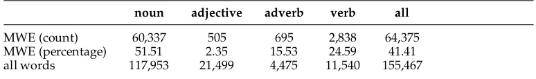
The detection of multiword units is one of the extensions needed for coarse-grained tokenization. As summarized concisely by Blanc, Constant, and Watrin (2007, page 1), “language is full of multiword units.” By inspecting dictionaries, we highlight the importance of MWEs. For example, in WordNet, 41.41% of all words are MWEs, as shown in Table 1. Whereas more than 50% of all nouns are MWEs, only about 26% of all verbs are MWEs. As the majority of all MWEs found in WordNet are nouns (93.73%), developing the method we focus first on the detection of terms belonging to this word class in Section 3.6 and show the performance on all word classes in subsequent sections. Although it seems intuitive to treat certain sequences of tokens as (single) terms, there is still considerable controversy about the definition of what exactly constitutes a MWE. Sag et al. (2001) pinpoint the need for an appropriate definition of MWEs. For this, they classify a range of syntactic formations that could form MWEs and define MWEs as being non-compositional with respect to the meaning of their parts. Although the exact requirements of MWEs is bound to specific tasks (such as parsing, keyword extraction, etc.), we operationalize the notion of non-compositionality by using distri-butional semantics and introduce a measure that works well for a range of task-based MWE definitions.

Reviewing previously introduced MWE ranking approaches (cf. Section 6.1), most methods use the following mechanisms to determine multiwordness: POS tags, word/multiword frequency, and significance of co-occurrence of the parts. In contrast, our method uses an additional mechanism, which performs a ranking based on distri-butional semantics.

Distributional semantics has already been used for MWE identification, but mainly to discriminate between compositional and non-compositional MWEs (Schone and Jurafsky 2001; Hermann and Blunsom 2014; Salehi, Cook, and Baldwin 2014). Here we introduce a concept to describe the multiwordness of a term by itsuniqueness. This score measures the likeliness that a term in context can be replaced with a single word. This measure is motivated by the semiotic consideration that due to parsimony, concepts are often expressed as single words. Furthermore, we deploy a context-aware punishment term, calledincompleteness, which degrades the score of candidates that seem incom-plete regarding their contexts. For example, the termred bloodcan be calledincompleteas the following word is most likely the wordcell. Both concepts are combined into a single score we callDRUID(DistRibutional Uniqueness and Incompleteness Degree), which is calculated based on a DT. In the following, we show the performance of this method for French and English and examine the effect of corpus size on MWE extraction. This section extends work presented in Riedl and Biemann (2015). In addition, we

Table 1

Amounts and percentages of MWEs contained in WordNet 3.1 for different POS.

noun adjective adverb verb all

MWE (count) 60,337 505 695 2,838 64,375

MWE (percentage) 51.51 2.35 15.53 24.59 41.41

demonstrate the language independence of the method by evaluating it on 32 languages and give a more detailed data analysis.

We want to emphasize that our method works in an unsupervised fashion and is not restricted to certain POS classes. However, most of the competitive methods require POS filtering as a pre-processing step in order to do their statistics. Hence, these methods are mostly evaluated based on noun compounds. Because of comparison reasons, the first evaluation that uses POS filtering (see Section 3.6) is restricted to noun compounds. However, the remaining experiments in Sections 3.7 and 3.8 are not restricted to any particular POS.

First, we describe the new method and show its performance on different data sets; we briefly describe the baseline and previous approaches in the next section.

3.1 Baselines and Previous Approaches

In the first setting, we evaluate our method by comparing the MWE rankings to mul-tiword lists that have been annotated in corpora. In order to show the performance of the method, we introduce an upper bound and two baseline methods and give a brief description of the competitors. Most of these methods rely on lists of pre-filtered MWE candidate termsT. Usually these are extracted by patterns defined on POS sequences.

3.1.1 Upper Bound.As an upper bound, we consider a perfect ranking, where we rank all positive candidates before all negative ones. Within the data set, we only have binary labels for true and false MWEs. Thus, any ordering of the MWEs within the block of MWEs labeled as true, respectively, false, does not change the upper bound.

3.1.2 Lower Baseline and Frequency Baseline. The ratio between true candidates and all candidates serves as a lower baseline, which is also called baseline precision (Evert 2008). The second baseline is the frequency baseline, which ranks candidate terms t∈Taccording to their frequencyfreq(t). Here, we hypothesize that words with high frequency are multiword expressions.

3.1.3 C-value/NC-value. Frantzi, Ananiadou, and Tsujii (1998) developed the commonly used C-value (see Equation (1)). This value is composed of two factors. As first factor, they use the logarithm of the term length in words in order to favor longer MWEs. The second factor is the frequency of the term reduced by the average frequency of all candidate terms T, which nest the termt (i.e.,t is a substring of the terms we denote asTt).

cv(t)=log₂(|t|)·



freq(t)− 1

|Tt|

X

b∈Tt

freq(b) 

 (1)

An extension of the C-value was proposed by Frantzi, Ananiadou, and Tsujii (1998) and is called the NC-value. It takes advantage of context wordsCt, which are neighboring

words oft, by assigning weights to them. As context words onlynouns,adjectives,and verbsare considered.3 _{Context words are weighted with Equation (2), wherekdenotes}

the number of times the context wordc∈Ctoccurs with any of the candidate terms.

This number is normalized by the number of candidate terms.

w(c)= k

|T| (2)

The NC-value is a weighted sum of the C-value and the product of the termtoccurring with each contextc, which form the termtc.

nc(t)=0.8·cv(t)+0.2X

c∈Ct

freq(tc)w(c) ₍₃₎

3.1.4 t-test.The t-test (see, e.g., Manning and Sch ¨utze 1999, page 163) is a statistical test for the significance of co-occurrence of two words. It relies on the probabilities of the term and its single words. The probability of a wordp(w) is defined as the frequency of the term divided by the total number of terms of the same length. The t-test statistic is computed using Equation (4) withfreq(.) being the total frequency of all unigrams.

t(w1. . .wn)≈ p(w1

. . .wn)−Qni=1p(wi)

p

p(w1. . .wn)/freq(.)

(4)

We then use this score to rank the candidate terms.

3.1.5 Marginal Frequency-Based Geometric Mean (FGM) Score. Nakagawa and Mori (2002, 2003) presented another method that is inspired by the C/NC-value and outperformed a modified C-value measure.4_{It is composed of two scoring mechanisms for the} candi-date termt, as shown in Equation (5).

FGM(t)=GM(t)·MF(t) (5)

The first term in the equation is the geometric meanGM(.) of the number of distinct direct leftl(.) and rightr(.) neighboring words for each single wordtiwithint.

GM(t)= 

 X

ti∈t

(|l(ti)|+1)(|r(ti)|+1)





1 2|t|

(6)

These neighboring words are extracted directly from the corpus; the method relies on neither candidate lists nor POS tags. In contrast, the marginal frequencyMF(t) relies on the candidate list and the underlying corpus. This frequency counts how often the candidate term occurs within the corpus and is not a subset of a candidate. Korkontzelos (2010) showed that although scoring according to Equation (5) leads to comparatively good results, it is consistently outperformed by the performance ofMF(t).

3.2 DistRibutional Uniqueness and Incompleteness Degree (DRUID)

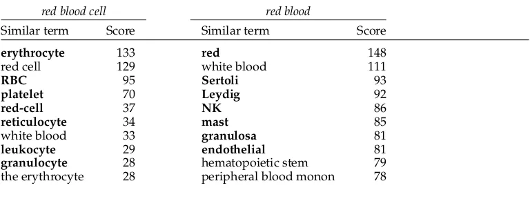
Here, we describe theDRUIDmethod for ranking terms regarding their multiwordness, which consists of two mechanisms relying on semantic word similarities: A score for theuniquenessof a term and a score that punishes itsincompleteness.5 The importance and influence of the results for the combination of both mechanisms is demonstrated in Section 3.9. The DT is computed as described in Section 2, usingn-grams (n=1, 2, 3, 4). When using JoBimText to compute such a DT, we use the left and right neighboring words as context. In order to compute the DRUID score using the CBOW model, we compute dense vector representations using word2vecf (Levy and Goldberg 2014) and convert it to a DT by extracting the 200 most similar words for eachn-gram. An example using JoBimText for the most similarn-grams to the termsred blood cell andred blood including their feature overlap is shown in Table 2.

3.2.1 Uniqueness Computation. The first mechanism of our MWE ranking method is based on the following hypothesis: n-grams that are MWEs could be substituted by single words, thus they have many single words among their most similar terms. When a semantically non-compositional word combination is added to the vocabulary, it expresses a concept that is necessarily similar to other concepts. Hence, if a candidate multiword is similar to many single word terms, this indicates multiwordness.

To compute theuniquenessscore (uq) of ann-gramt, we first extract then-grams it is similar to using the DT as described in Section 2. The functionsimilarities(t) returns the 200 most similarn-grams to the given n-gramt. We then compute the ratio between unigrams and all similar n-grams considered using the formula, where the function unigram(.) tests whether a word is a unigram:

uq(t)= |{∀w∈similarities(t)|unigram(w)}|

|similarities(t)| . (7)

We illustrate the computation of our measure based on two example terms: the MWE red blood cell and the non-MWEred blood. When considering only the ten most similar entries for both n-grams as illustrated in Table 2, we observe a uniqueness score of 7/10=0.7 for both n-grams. If considering the top 200 similar n-grams, which are also used in our experiments, we obtain 135 unigrams for the candidatered blood cell and 100 unigrams for the n-gramred blood. We use these counts for exemplifying the workings of the method in the remainder.

3.2.2 Incompleteness Computation. In order to avoid ranking nested terms at high positions, we introduce a measure that punishes such “incomplete terms”. This mecha-nism is called incompleteness (ic) and, similarly to the C/NC-value method (see Section 3.1.3), consists of a context weighting function that punishes incomplete terms. We show the pseudocode for the computation in Algorithm 1. First, we use the function context(t) to extract the 1,000 most significant context features. This function returns a list of tuples of left and right contexts.

5 TheDRUIDimplementation is available open source and pre-computed models can be found here:

Table 2

The ten most similar entries for the termred blood cell(left) andred blood(right). Here, seven of ten terms are single words in both lists.

red blood cell red blood

Similar term Score Similar term Score

erythrocyte 133 red 148

red cell 129 white blood 111

RBC 95 Sertoli 93

platelet 70 Leydig 92

red-cell 37 NK 86

reticulocyte 34 mast 85

white blood 33 granulosa 81

leukocyte 29 endothelial 81

granulocyte 28 hematopoietic stem 79

the erythrocyte 28 peripheral blood monon 78

Algorithm 1Computation of the incompleteness score 1: functionic(t)

2: contexts←context(t) 3: C←map()

4: for all(cleft,cright)incontextsdo

5: C[cleft,left]←C[cleft,left]+1

6: C[cright,right]←C[cright,right]+1

7: end for

8: returnmax value(C)/|contexts|

9: end function

For JobimText, these context features are the same that are used for the similarity computation in Section 2 and have been ranked according to the LMI measure. In the case of word2vecf, context features are extracted per word. To be compatible with the JoBimText contexts, we extract the 1,000 contexts with the highest cosine similarity between word and context.

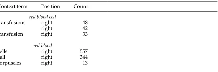
For the example term red blood, some of the contexts are hextravasated, cellsi,

huninfected, cellsi, hnucleated, corpusclesi. In the next step we iterate over all contexts. Using the first context feature results in the tuple(extravasated, cells). Then, we sepa-rately count the occurrence of both the left and the right context, including its relative position (left/right) as illustrated in Table 3 for the two example terms.

We subsequently return the maximal count and normalize it by the counts of fea-tures|context(t)|considered, which is at most 1,000. This results in the incompleteness measureic(t). For our example terms we achieve the valuesic(red blood)=557/1, 000 and ic(red blood cell)=48/1, 000. Whereas the uniqueness scores for the most similar entries are close together (100 vs. 135), we now have a measure that indicates the incompleteness of ann-gram, assigning higher scores to more incomplete terms.

Table 3

Top three most frequent context words for the termred blood cellandred bloodin the Medline corpus.

Context term Position Count

red blood cell

transfusions right 48

( right 42

transfusion right 33

red blood

cells right 557

cell right 344

corpuscles right 13

the overall score. In our experiments (see Section 3.9) we reveal that using solely the uniquenessscore results in good scores. However, often expressions ending with stopwords and incomplete MWEs are detected. In experiments, we found the best combination when we subtract the incompleteness score from the uniqueness score.6 This mechanism is inspired by the NC-value and motivated as terms that are often preceded/followed by the same word do not cover the full multiword expression and need to be downranked. This leads to Equation (8), which we callDistRibutional Uniqueness andIncompletenessDegree:

DRUID(t)=uq(t)−ic(t) (8)

Applying the DRUID score to our example terms (considering the 200 most similar terms) we achieve the scores DRUID(red blood cell)=135/200−48/1, 000=0.627 and DRUID(red blood)=100/200−557/1, 000=−0.057. As a higher DRUID score indicates the multiwordness of ann-gram, we conclude that then-gramred blood cellis a better MWE than then-gramred blood.

3.3 Experimental Setting

To evaluate the method, we examine two experimental settings: first, we compute all measures on a small corpus that has been annotated for MWEs, which serves as the gold standard. In the second setting, we compute the measures on a larger in-domain corpus. The evaluation is again performed for the same candidate terms as given by the gold standard. Results for the topkranked entries are reported using the precision atk:

P@k= 1

k

k

X

i=1

xi (9)

withxi equal to 1 if theith ranked candidate is annotated as MWE and 0 otherwise.

For an overall performance we use the average precision (AP) as defined by Thater, Dinu, and Pinkal (2009):

AP= 1

|Tmwe|

|T|

X

k=1

xkP@k (10)

withTmwebeing the set of positive MWEs. When facing tied scores, we mix false and

true candidates randomly following Cabanac et al. (2010).

3.4 Corpora

For the first experiments, we consider two annotated (small) corpora and two unan-notated (large) corpora for the evaluation and computation of MWEs. The language independence ofDRUIDis demonstrated on various Wikipedia text corpora.

GENIA Corpus and SPMRL 2013: French Treebank.In the first experiments, we use two small annotated corpora that serve as the gold standard MWEs. We use the medical GENIA corpus (Kim et al. 2003), which consists of 1,999 abstracts from Medline7 _and encompasses 0.4 million words. This corpus has annotations regarding important and biomedical terms.8 _{In addition, single terms are annotated in this data set, which we} ignore.

The second small corpus is based on the French Treebank (Abeill´e and Barrier 2004), which was extended for the SPMRL task (Seddah et al. 2013). This version of the corpus also contains compounds annotated as MWEs. In our experiments, we use the training data, which cover 0.4 million words.

Whereas the GENIA MWEs target term matching and medical information re-trieval, the SPMRL MWEs mainly focus on improving parsing through compound recognition.

Medline Corpus and Est R´epublicain Corpus (ERC).In a second experiment, the scalability to larger corpora is tested. For this, we make use of the entire set of Medline ab-stracts, which consists of about 1.1 billion words. The Est R´epublicain Corpus (Seddah et al. 2012) is our large French corpus.9 It is made up from local French newspapers from the eastern part of France and comprises 150 million words.

Wikipedia.Applying the methods to texts extracted from 32 Wikipedias validates their language independence. For this, we use the following languages: Arabic, Basque, Bulgarian, Catalan, Croatia, Czech, Danish, Dutch, English, Estonian, Finnish, French, Galician, German, Greek, Hebrew, Hungarian, Italian, Kazakh, Latin, Latvian, Nor-wegian, Persian, Polish, Portuguese, Romanian, Russian, Slovene, Spanish, Swedish, Turkish, and Ukrainian.

7 The Medline corpus is available at:

http://www.nlm.nih.gov/bsd/licensee/access/medline_pubmed.html. 8 The GENIA corpus is freely available at:

3.5 Candidate Selection

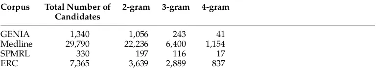
In the first two experiments, we use POS filters to select candidates. We concentrate on filters that extract noun MWEs, as they constitute the largest number of MWEs (see Table 1) and avoid further preprocessing like lemmatization. We use the filter introduced by Justeson and Katz (1995) for the English medical data sets (see Table 4).

Considering only terms that appear more than ten times yields 1,340 candidates for the GENIA data set and 29,790 candidates for the Medline data set. According to Table 5, we observe that most candidates are bigrams. Whereas about 20% of MWEs are trigrams in both corpora, only a marginal number of longer MWEs have been marked.

For the French data sets, we apply the POS filter proposed by Daille, Gaussier, and Lang´e (1994), which is suited to match nominal MWEs (see Table 4). Applying the same filtering as for the medical corpora leads to 330 candidate terms for the SPMRL and 7,365 candidate terms for the ERC. Here the ratio between bigrams and trigrams is more balanced but again the number of 4-grams constitutes the smallest class.

In comparison with the Medline data set, the ratio of multiwords extracted by the POS filter on the French corpus is much lower. We attribute this to the fact that in the French data, many adverbial, prepositional MWEs are annotated, which are not covered by the POS filter.

The third experiment shows the performance of the method in absence of language-specific preprocessing. Thus, we only filter the candidates by frequency and do not make use of POS filtering. As most previous methods rely on POS-filtered data, we cannot compare with them in this language-independent setting.

For the evaluation, we compute the scores of the competitive methods in two ways: First, we compute the scores based on the full candidate list without any frequency filter and prune low-frequent candidates only for the evaluation (post-prune). In the second setting, we filter candidates according to their frequency before the computation

Table 4

POS sequences for filtering noun MWEs for English and French. Each letter is a truncated POS tag of length one whereJis an adjective,Na noun,Pa preposition, andDa determiner.

Language POS filter

English (Korkontzelos 2010) (([JN]+[JN]?[NP]?[JN]?)N)

French (Daille, Gaussier, and Lang´e 1994) N[J]?|NN|NPDN

Table 5

Number of MWE candidates after filtering for the expected POS tag. Additionally, the table shows the distribution overn-grams withn∈ {1, 2, 3, 4}.

Corpus Total Number of 2-gram 3-gram 4-gram Candidates

GENIA 1,340 1,056 243 41

Medline 29,790 22,236 6,400 1,154

SPMRL 330 197 116 17

of scores (pre-prune). This leads to differences for context-aware measures, because in the pre-pruned case a lower number of less noisy contexts is used.

The evaluation on Wikipedia is slightly different, as we do not have any gold data. Thus, we compute the ranking regarding the multiwordness for all words in the corpus. Based on this list, we determine the multiwordness of ann-gram by testing its existence in the respective language’s Wiktionary.

3.6 Results Using POS

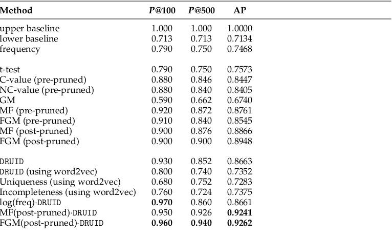
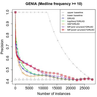
First, we present the results based on the GENIA corpus (see Table 6). Almost all competitive methods beat the lower baseline. The C/NC-value performs best when the pruning is done after the frequency filtering. In line with the findings of Korkontzelos (2010) and in contrast to Frantzi, Ananiadou, and Tsujii (1998), the AP of the C-value is slightly higher than for the NC-value. All the FGM-based methods except the GM measure alone outperform the C-value. The results in Table 6 indicate that the best com-petitive system is the post-pruned FGM system, as it has much higher average precision scores and misses only 50 MWEs in the first 500 entries. A slightly different picture is presented in Figure 1, where we plot theP@kscores against the number of candidates. Here DRUID computed on the JoBimText similarities performs well for the top-k list for smallk, that is, it finds many valid MWEs with high confidence, thus combines well with MF, which extends to largerk, but places too much importance of frequency when used alone. Common errors occur for frequent prepositional phrases, such as

Table 6

Results for P@100, P@500, and the average precision (AP) for various ranking measures. The gold standard is extracted using the GENIA corpus. This corpus is also used for computing the measures.

Method P@100 P@500 AP

upper baseline 1.000 1.000 1.0000

lower baseline 0.713 0.713 0.7134

frequency 0.790 0.750 0.7468

t-test 0.790 0.750 0.7573

C-value (pre-pruned) 0.880 0.846 0.8447 NC-value (pre-pruned) 0.880 0.840 0.8405

GM 0.590 0.662 0.6740

MF (pre-pruned) 0.920 0.872 0.8761

FGM (pre-pruned) 0.910 0.840 0.8545

MF (post-pruned) 0.900 0.876 0.8866

FGM (post-pruned) 0.900 0.900 0.8948

DRUID 0.930 0.852 0.8663

DRUID(using word2vec) 0.800 0.740 0.7352

Uniqueness (using word2vec) 0.680 0.752 0.7283 Incompleteness (using word2vec) 0.760 0.724 0.7375

log(freq)·DRUID 0.970 0.860 0.8661

0

200

400

600

800

1000

1200

0.6

0.7

0.8

0.9

1.0

GENIA (GENIA frequency >= 10)

Number of instances

Precision

● ● ● ● ● ● ● ● ● ● ● ● ● ● ●

●

●

●

●

●

●

● _{upper baseline} lower baseline MF (post−pruned) FGM (post−pruned)

DRUID

log(freq)*(DRUID) MF(post−pruned)*DRUID FGM(post−pruned)*DRUID

Figure 1

This graph shows the P@k for some measures, plotting the precision againstk. UsingDRUIDin combination with the MF and FGM measures yields the highest precision scores.

When looking at effects between post-pruning and pre-pruning, we observe that FGM scores higher than MF when post-pruning, but the inverse is observed when pre-pruning. Our JoBimText-basedDRUID method can outperform FGM only on the top-ranked 300 terms (see Figure 1 and Table 6).

Multiplying the logarithmic frequency with DRUID, the results improve slightly and the bestP@100 of 0.97 is achieved. All FGM results are outperformed when com-bining the post-pruned FGM scores with our measure. According to Figure 1, this combination achieves high precision for the first ranked candidates and still exploits the good performance of the post-pruned FGM based method for the middle-ranked candidates.

Different results are achieved for the SPMRL data set, as can be seen in Table 7. Whereas the pre-pruned C-value again receives better results than frequency, it scores below the lower baseline. In addition, the post-pruned FGM and MF method do not exceed the lower baseline. Data analysis revealed that for the French data set only ten out of the 330 candidate terms are nested within any of the candidates. This is much lower than the 637 terms nested in the 1340 candidate terms for the GENIA data set. As both the FGM-based methods and the C/NC-value heavily rely on nested candidates, they cannot profit from the candidates of this data set and achieve similar scores as ordering candidates according to their frequency. Comparing the baselines to our scoring method, this time we obtain the best result forDRUID without additional factors. However, multiplyingDRUID with MF or log(frequency) still outperforms the other methods and the baselines.

Most MWE evaluations have been performed on rather small corpora. Here, we examine the performance of the measures for large corpora, to realistically simulate a situation where the MWEs should be found automatically for an entire domain or language.

Using the Medline corpus, all methods except the GM score outperform the lower baseline and the frequency baseline (see Table 8). Regarding the AP the best results are obtained when combining our DRUID method with the MF, whereas for P@100 and P@500 the log-frequency-weighted DRUID scores best. As we can observe from

Table 7

Results for MWE detection on the French SPMRL corpus. Both the generation of the gold standard and the computations of the measures have been performed on this corpus.

Method P@100 P@200 AP

upper baseline 1.000 0.860 1.0000

lower baseline 0.521 0.521 0.5212

frequency 0.500 0.480 0.4876

t-test 0.500 0.485 0.4934

C-value (pre-pruned) 0.490 0.540 0.5107 MF (post-pruned) 0.510 0.495 0.5017 FGM (post-pruned) 0.460 0.480 0.4703

DRUID 0.790 0.690 0.7794

Table 8

Results ofn-gram ranking on the medical data. Whereas the gold standard is extracted from the GENIA data set, the ranking measures as well as the frequency threshold for selecting the gold candidates are computed using the Medline corpus.

Method P@100 P@500 AP

upper baseline 1.000 1.000 1.0000 lower baseline 0.416 0.416 0.4161

frequency 0.720 0.534 0.4331

C-value (pre-pruned) 0.750 0.564 0.4519

t-test 0.720 0.542 0.4483

GM 0.210 0.272 0.3502

MF (pre-pruned) 0.550 0.542 0.4578 FGM (pre-pruned) 0.580 0.478 0.4200 MF (post-pruned) 0.530 0.500 0.4676 FGM (post-pruned) 0.490 0.446 0.4336

DRUID 0.770 0.686 0.4608

log(freq)·DRUID 0.860 0.720 0.4693

GM·DRUID 0.770 0.634 0.4497

MF(pre-pruned)·DRUID 0.730 0.634 0.4824 MF(post-pruned)·DRUID 0.730 0.626 0.4889

Figure 2, using solely the DRUID method or the combined variation with the log-frequency lead to the best ranking for the first 1,000 ranked candidates. However, both methods are outperformed beyond the first 1,000 ranked candidates by the MF-informed DRUID variations. Using the combination with GM results in the lowest scores.

In this experiment, the C-value achieves the best performance from the competitive methods for theP@100 andP@500, followed by the t-test. But the highest AP is reached with the post-pruned MF method, which also outperforms the sole DRUID slightly. Contrary to the GENIA results, the MF scores are consistently higher than the FGM scores.

In the French ERC, no nested terms are found within the candidates. Thus, the post-pruned and pre-pruned settings are equivalent and thus MF equals frequency. We show the results for the evaluation using the ERC in Table 9.

The best results are again obtained with our method with and without the loga-rithmic frequency weighting. Again, the AP of the C-value and most of the FGM-based methods are inferior to the frequency scoring. Only the t-test and the MF score slightly higher than the frequency.10In contrast to the results based on the smaller SPMRL data set, the MF, FGM, and C-value can outperform the lower baseline.

In comparison to the smaller corpora, the performance for the larger corpora is much lower. Especially low-frequent terms in the small corpora that have high frequen-cies in the larger corpora have not been annotated as MWEs.

0

5000

10000

15000

20000

25000

0.4

0.5

0.6

0.7

0.8

0.9

1.0

GENIA (Medline frequency >= 10)

Number of instances

Precision

● ● ● ● ● ● ● ● ●

●

●

●

●

●

●

●

● ●

● ●

● ● _{upper baseline}

lower baseline DRUID

log(freq)*DRUID GM*DRUID

MF(pre−pruned)*DRUID MF(post−pruned)*DRUID

Figure 2

Precision scores when considering different number of highest ranked words forDRUIDand combinedDRUIDvariations. Here, the gold standard is extracted from the GENIA data set, whereas the scores for the methods are computed using the Medline corpus.

3.7 Results Without POS Filtering

Next, we apply our method to candidates without any POS filtering and report results for candidates surpassing a frequency threshold of 10. Thus, we do not only restrict the evaluation on noun MWEs but use all MWEs of all POS classes that have been annotated in both corpora. As most competitive methods from the previous section rely on POS tags, we only use the t-test for comparison.

Table 9

Results for rankingn-grams, according to their multiwordness, based on the French ERC. The candidates are extracted based on the smaller SPMRL corpus.

Method P@100 P@500 AP

upper baseline 1.000 1.000 1.0000 lower baseline 0.220 0.220 0.2201 frequency 0.370 0.354 0.3105

C-value 0.420 0.366 0.3059

t-test 0.390 0.360 0.3134

GM 0.010 0.052 0.1694

MF 0.370 0.356 0.3148

FGM 0.280 0.260 0.2405

DRUID 0.700 0.568 0.3962

log(freq)·DRUID 0.760 0.582 0.4075

MF·DRUID 0.570 0.516 0.3776

FGM·DRUID 0.510 0.418 0.3234

Table 10

MWE ranking results based on different methods without using any linguistic preprocessing.

Corpora Method Medical French

P@100 AP P@100 AP

small

corpora

upper baseline 1.000 1.0000 1.000 1.0000 lower baseline 0.107 0.1071 0.083 0.0832

frequency 0.150 0.1135 0.060 0.0906

t-test 0.160 0.1261 0.080 0.1097

t-test + sw 0.530 0.3643 0.180 0.1481

DRUID 0.700 0.4048 0.670 0.2986

log(freq)·DRUID 0.690 0.3644 0.460 0.2527

lar

ge

corpora

upper baseline 1.000 1.0000 1.000 1.0000 lower baseline 0.036 0.0361 0.019 0.0191

frequency 0.010 0.0361 0.060 0.0366

t-test 0.020 0.0412 0.080 0.0440

t-test + sw 0.000 0.0989 0.200 0.0485

DRUID 0.610 0.1378 0.660 0.1009

log(freq)·DRUID 0.760 0.1649 0.600 0.0988

3.8 Multilingual Evaluation

In order to demonstrate the performance ofDRUID for several languages, we perform an evaluation on 32 languages. For this experiment, we compute similarities on their respective Wikipedias.11 The evaluation is performed by extracting the 1,000 highest ranked words usingDRUID. In order to determine whether a word sequence is a MWE, we use Wiktionary as “gold” standard and test whether it occurs as word entry.12_Using this information, we compute the AP for these 1,000 ranked words.

We present the results for this experiment in columns 2 to 5 in Table 11. The t-test with stopword filtering mostly performs similar to the frequency baseline and improves from an average score of 0.07 to 0.08. We observe that in comparison to two baselines, frequency (freq.) and the t-test with stopword filtering, theDRUIDmethod yields the best scores for 6 out of the 32 languages. However, if we multiply the logarithmic frequency by the DRUID measure, we gain the best performance for 30 languages. In general, numerical scores are low—for example, for Arabic, Slovene, or Italian, we obtain APs below 0.10. The highest scores are achieved for Swedish (0.33), German (0.36), Turkish (0.36), French (0.44), and English (0.70). Analyzing the results, we observe that many “false” MWEs are multiword units that are in fact multiword units, which are just not covered in the respective language’s Wiktionary. Furthermore, we detect that these word sequences often are titles of Wikipedia articles. The absence of word lemmatiza-tion causes further decline, as words in Wiklemmatiza-tionary are recorded in lemmatized form. To alleviate this influence, we extend our evaluation and check the occurrence of word sequences both in Wiktionary and Wikipedia. Using the Wikipedia API also normalizes query terms and, thus, we obtain a better word sequence coverage. This is confirmed by much higher results, as shown in columns 6 through 9 in Table 11. Using the frequency combination withDRUID, we even gain higher APs for languages, which attained worse scores in the previous setting (e.g., Arabic [0.62], Slovene [0.17], and Italian [0.44]). Except for Estonian and Polish, using the logarithmic frequency weighting performs best for all languages. For these two languages, using the soleDRUIDmeasure performs best. The best performance is obtained for English (0.87), Turkish (0.66), French (0.66), German (0.62), and Portuguese (0.64). Based on these multilingual experiments, we have demonstrated thatDRUIDnot only performs well for English and French, but also for other languages, showing that its elements, uniqueness and incompleteness, are language-independent principles for multiword characterization.

3.9 Components ofDRUID

Here, we show different parameters for DRUID, relying on the English GENIA data set without POS filtering of MWE candidates and by considering only terms with a frequency of 10 or more. Inspecting the two different components of theDRUIDmeasure (see Figure 3 top), we observe that the uniqueness measure contributes most to the DRUIDscore. The main effect of the incompleteness component is the downranking of a rather small number of terms with high uniqueness scores, which improves the overall

11 We use Wikipedia dumps from late 2016.

Table 11

AP for the frequency baseline, t-test, andDRUIDevaluated against Wiktionary and a combination of Wiktionary and Wikipedia, including word normalization.

Language Wiktionary Wiktionary & Wikipedia

freq t-tests DRUID log(freq)· freq t-test DRUID log(freq)·

+sw DRUID +sw DRUID

Arabic 0.01 0.01 0.00 0.01 0.27 0.30 0.32 0.62

Basque 0.01 0.01 0.01 0.03 0.05 0.06 0.33 0.23

Bulgarian 0.01 0.01 0.00 0.03 0.28 0.35 0.23 0.54

Catalan 0.02 0.02 0.06 0.07 0.13 0.18 0.29 0.39

Croatia 0.04 0.05 0.01 0.06 0.14 0.15 0.11 0.21

Czech 0.07 0.07 0.01 0.08 0.17 0.20 0.14 0.28

Danish 0.01 0.02 0.01 0.25 0.19 0.21 0.19 0.32

Dutch 0.09 0.11 0.05 0.18 0.20 0.25 0.27 0.53

English 0.10 0.49 0.21 0.70 0.19 0.54 0.56 0.87

Estonian 0.03 0.03 0.03 0.05 0.12 0.13 0.17 0.14

Finnish 0.14 0.12 0.02 0.11 0.11 0.11 0.16 0.19

French 0.17 0.18 0.21 0.44 0.30 0.32 0.38 0.66

Galician 0.12 0.10 0.03 0.12 0.29 0.29 0.19 0.42

German 0.25 0.23 0.07 0.36 0.28 0.27 0.40 0.65

Greek 0.07 0.08 0.04 0.08 0.14 0.17 0.15 0.26

Hebrew 0.05 0.06 0.01 0.12 0.27 0.31 0.05 0.34

Hungarian 0.09 0.10 0.03 0.20 0.14 0.16 0.09 0.29

Italian 0.10 0.10 0.01 0.10 0.28 0.30 0.06 0.44

Kazakh 0.01 0.01 0.01 0.05 0.07 0.08 0.27 0.32

Latin 0.01 0.01 0.04 0.09 0.09 0.11 0.13 0.28

Latvian 0.00 0.00 0.00 0.01 0.10 0.10 0.07 0.13

Norwegian 0.02 0.02 0.39 0.21 0.19 0.20 0.28 0.40

Persian 0.08 0.11 0.04 0.19 0.29 0.37 0.41 0.55

Polish 0.07 0.08 0.02 0.19 0.12 0.14 0.36 0.32

Portuguese 0.14 0.14 0.05 0.20 0.31 0.34 0.32 0.64

Romanian 0.05 0.06 0.05 0.16 0.20 0.25 0.19 0.47

Russian 0.07 0.07 0.02 0.15 0.16 0.17 0.16 0.27

Slovene 0.01 0.01 0.01 0.05 0.09 0.11 0.09 0.17

Spanish 0.12 0.14 0.02 0.12 0.34 0.42 0.26 0.63

Swedish 0.07 0.10 0.03 0.33 0.19 0.26 0.42 0.58

Turkish 0.08 0.10 0.20 0.36 0.20 0.22 0.50 0.66

Ukrainian 0.01 0.01 0.02 0.04 0.09 0.11 0.12 0.14

Average 0.07 0.08 0.05 0.16 0.19 0.22 0.24 0.40

ranking. We can also see that for the top-ranked terms, the negative incompleteness score does not improve over the frequency baseline but merely outperforms frequency for candidates in the middle range. Used inDRUID, we observe a slight improvement for the complete ranking.

We achieve a P@500 of 0.474 for the uniqueness scoring and 0.498 for the DRUID score.

0 2000 4000 6000 8000 10000

0.0

0.2

0.4

0.6

0.8

1.0

GENIA (GENIA frequency >= 10)

Number of instances

Precision

● ● ●

●

●

●

● ●

● ●

● _● ● ●

● ● ● _{● ● ● ●}

● upper baseline lower baseline frequency DRUID UQ −IC

0 2000 4000 6000 8000 10000

0.0

0.2

0.4

0.6

0.8

1.0

GENIA frequency >= 10 and no POS filter

Number of instances

Precision

● ● ●

●

●

●

● ●

● ●

● _● ● ●

● ● ● _{● ● ● ●}

● upper baseline lower baseline frequency

number of single similarities > 0 number of single similarities > 5 number of single similarities > 10 number of single similarities > 20

Figure 3

3.10 Discussion and Data Analysis

The experiments confirm that ourDRUIDmeasure, either weighted with the MF or alone, works best across two languages and across different corpus sizes. It also achieves the best results in absence of POS filtering for candidate term extraction. The optimal weighting ofDRUIDdepends on the nestedness of the MWEs: UsingDRUIDwith the MF should be applied when there are more than 20% of nested candidates. If there are no nested candidates, we recommend using the log-frequency or no frequency weighting.

We present the best-ranked candidates obtained with our method and with the best competitive method in terms ofP@100 for the two smaller corpora. Using the GENIA data set, our log-frequency basedDRUID (see left column in Table 12) ranks only true MWE within the 15 top-scored candidates.

The right-hand side shows results extracted with the pre-pruned MF method that yields three non-MWE terms. Whereas these terms seem to be introduced as candidates due to a POS error, the MF, and the C-value are not capable of removing terms starting with stopwords. The DRUID score alleviates this problem with the uniqueness factor. For the French data set, only one false candidate is ranked in the top 15 candidates.

In comparison, eight non-annotated candidates are ranked in the top 15 candidates by the MF (post-pruned) method as shown in Table 13.

Whereas the unweightedDRUID method scores better than its competitors on the large corpora, the best numerical results are achieved when usingDRUIDwith frequency-based weights on smaller corpora. For a direct comparison, we evaluated the small and large corpora using an equal candidate set. We observed that all methods computed on the large corpora achieve slightly inferior results than when computing them using the small corpora.

Data analysis revealed that we personally would consider many of these high ranked “false” candidates as MWEs.

For examining the effect, we extracted the top ten ranked terms, which are not annotated as MWE from the methods with the best P@100 performance, resulting in

Table 12

Top ranked candidates from the GENIA data set using our ranking method (left) and the competitive method (right). Each term is marked if it is an MWE (1) or not (0).

log(freq)·DRUID MF (pre-pruned)

NF-kappa B 1 T cells 1

transcription factors 1 NF-kappa B 1

transcription factor 1 transcription factors 1

I kappa B alpha 1 activated T cells 1

activated T cells 1 T lymphocytes 1

nuclear factor 1 human monocytes 1

human monocytes 1 I kappa B alpha 1

gene expression 1 nuclear factor 1

T lymphocytes 1 gene expression 1

NF-kappa B activation 1 NF-kappa B activation 1

binding sites 1 in patients 0

MHC class II 1 important role 0

tyrosine phosphorylation 1 binding sites 1

transcriptional activation 1 in B cells 0

Table 13

Top ranked candidates from the SPMRL data set for the bestDRUIDmethod (left) and the best competitive method (right). Each term is marked if it is an MWE (1) or not (0).

DRUID MF (post-pruned)

hausse des prix 1 milliards de francs 0

mise en oeuvre 1 millions de francs 0

prise de participation 1 Etats - Unis 1 chiffre d’ affaires 1 chiffre d’ affaires 1 formation professionnelle 1 taux d’ int´erˆet 1 population active 1 milliards de dollars 0 taux d’ int´erˆet 1 millions de dollars 0

politique mon´etaire 1 Air France 1

Etats - Unis 1 % du capital 0

R´eserve f´ed´erale 1 milliard de francse 0 comit´e d’ ´etablissement 1 directeur g´en´eral 1

projet de loi 1 M. Jean 0

syst`eme europ´een 0 an dernier 1

conseil des ministres 1 ann´ees 1

Europe centrale 1 % par rapport 0

Table 14

Top ranked terms for the Medline corpus, which are not marked as MWEs. The rank is denoted to the left of each term and all terms, which can be found within a lexicon, are marked inbold.

log(freq)DRUID C-value (pre-pr.)

26 carboxylic acid 1 present study 28 connective tissue 7 important role

40 cathepsin B 11 degrees C

41 soft tissue 13 risk factors

42 transferrin receptor 15 significant differences

53 DNA damaging 18 other hand

61 foreign body 22 significant difference 62 radical scavenging 33 magnetic resonance 71 spatial distribution 39 first time

74 myosin heavy chain 48 significant increase

the log(freq)DRUIDand the pre-pruned C-value methods. We show the terms including their ranking position based on the GENIA data set in Table 14.

First, we observe that the first “false” candidate for our method appears at rank 26 and at rank 1 for the C-value. Additionally, only 10 out of the top 74 candidates are not annotated as MWEs for our method, whereas the same number of 10 non-MWEs is found in the first 48 candidates for the competitor. When searching the terms within the MeSH dictionary, we find seven terms ranked from our method and two for the competitive method, showing that most such errors are at least questionable, given that these terms are contained in a domain-specific lexicon.13This leads us to the conclusion that our method scales to larger corpora.

Table 15

The highest ranked single-worded terms for Medline and ERC without any POS filtering, based on theDRUIDscore.

Medline ERC

GATA-1 antiatherosclerotic mesure Berg´e

function Smad6 activit´es carnets

Sp1 Evi-1 politique Bouvet

used ETS1 prix promesse

increased 3q26 r´eduction pr´eoccupe

shown Tcf analyse composants

IFN-gamma LEF-1 crise aspirations

decreased hypolipidaemic strat´egie hostilit´e

IL-10 down-regulatory tˆete dettes

IL-5 Xq13 campagne Brunet

In contrast to the competitive measures introduced in this section, our method is also able to rank single-worded terms. We show the 20 highest ranked single-worded terms in Table 15 for the Medline and the ERC corpus. In both lists we did not filter by POS and removed numbers, which often have a highDRUIDscore. Both for French and for the medical data, we observe some verbs, but mostly common and proper nouns. These are well suited as keyword lists that are required for document indexing used, e.g., for search engines or automatic speech recognition, as we have demonstrated in Milde et al. (2016).

3.11 Summary on MWE Identification

frequently we observe single n-grams with function words or modifying adjectives concatenated with content words—for example,small dogis most similar to “various cat”, “large amount of”, “large dog”, “certain dog”, and “dog”. To be able to kick in, the measure requires a certain minimum frequency for candidates in order to find enough contextual overlap with other terms. Additionally, we demonstrate effective performance on larger corpora and show its applicability when used in a completely unsupervised evaluation setting. Furthermore, we have demonstrated the language independence of the measure by evaluating it on 32 languages using Wiktionary and Wikipedia for the evaluation.

4. Splitting Words: Decompounding

In order to enable a tokenization for sub-word units, we introduceSECOS (SEmantic COmpound Splitter), which is based on the hypothesis that compounds are similar to their constituting word units.14_{Again, our method is based on a DT. In addition, it does} not require any language-specific rules and can be applied in a knowledge-free way. We exemplify the method based on the compound nounBundesfinanzministerium(federal finance ministry), which is assembled of the wordsBundes(federal),Finanz(finance), and Ministerium(ministry). This section extends the work presented in Riedl and Biemann (2016) by adding results on an Afrikaans and a Finnish data set. Additionally, we introduce an evaluation based on automatically extracted compounds from Wiktionary and present results for 14 languages.

4.1 SEmantic COmpound Splitter (SECOS)

Our method consists of three stages: First, we extract a candidate word set that defines the possible sub-word units of compounds. We present several approaches to generate such candidates. Second, we use a general method that splits the compound based on a candidate word set. Using different candidate sets, we obtain different compound splits. Finally, we define a mechanism that ranks these splits and returns the top-ranked one.

Candidate Extraction. For the extraction of all candidates in C, we use a DT that is computed on a background corpus. We present three approaches for the generation of candidate sets.

When we retrieve thelmost similar terms for a wordwfrom a DT, we observe well-suited candidates that are nested inw. For example,Bundesfinanzministeriumis similar to Bund,Bundes, andFinanzministerium. Extracting the most similar terms that are nested inw results in the first split candidate set, called similar candidate units. However, only for few terms do we observe nested candidates in the most similar words. Thus, we require methods to generate “back-off” candidates.

First, we introduce the extended similar candidate units. Here, we extract thel most similar terms forwand then grow this set by again adding their respectivelmost similar words. Based on these terms, we extract all words that are nested inw. This results in more but less-precise decompounding candidates.

As the coverage might still be insufficient to decompound all words (e.g., entirely unseen compounds), we propose a method to generate a global dictionary of single

atomic word units. For this, we iterate over the entire vocabulary of the background corpus, applying the compound splitter (see Section 4.1) to all words where we find similar candidate units. Then, we add these detected units to the dictionary. Finally, for wordwsubject to decompounding, we first extract all nested wordsNWfrom this dictionary. Then, we remove all words inNWthat are nested itself inNW, resulting in the candidate set we callgenerated dictionary.

Compound Splitting.Here, we introduce the decompounding algorithm for a given can-didate set. For decompounding the wordw, we require a set of candidate wordsC. Each word in the candidate set needs to be a substring ofw. We do not include candidates in Cthat have less thanmlcharacters. Additionally, we apply a frequency threshold ofwc. These mechanisms are intended to rule out spurious parts and “words” that are in fact short abbreviations.

We show candidates, extracted from the similar candidate unit, with ml=3 for the example term in Table 16. Then, we iterate over each candidateci∈Cand add its

beginning and ending position withinwto the setS. This set is then used to identify possible split positions of w. For this, we iterate from left to right and add all split possibilities to the wordw. This approach overgenerates split points, as can be observed for the example word, which is split into six units:Bund-e-s-finanz-minister-ium.

To merge charactern-grams, we use a suffix- and prefix-based method. The suffix merging method appends all charactern-grams withnbelowmsto the left word. The prefix method merges all charactern-grams withnbelowmpto the word on the right side. To avoid remaining prefixes/suffixes, we apply the opposite method afterwards. For the German language, the suffix-prefix ordering mostly yields the best output. The suffix-prefix-based approach results to Bundes-finanz-ministerium and the prefix-suffix method toBund-esfinanz-ministerium. However, for some words, the prefix-suffix generates the correct compound split—for example, for the wordZuschauer-er-wartung (audience + he + service), which is correctly decompounded as Zuschauer-erwartung (audience+expectation).

In order to select the correct split, we compute the geometric mean of the joint probability for each split variation. For this we use word counts from a background corpus. In addition to the geometric mean formula introduced in Koehn and Knight (2003), we add a smoothing factor to each frequency in order to assign non-zero

Table 16

Examples of the output of our algorithms for the example termBundesfinanzministerium.

wordw Bundesfinanzministerium

candidatesC Finanzministerium, Ministerium, withml=3 Bunde, Bund, Bundes, Minister split possibilities Bund-e-s-finanz-minister-ium

Merging charactern-grams

values to unknown units.15_{This yields the following formula for a compoundw, which} is decomposed into the unitsw1,. . .,wN:

p(w)=

N

Y

i

wordcount(wi)+

total wordcount+·#words

!N1

(11)

Here, #word denotes the total number of words in the background corpus and total wordcountis the sum of all word counts. Then, we select the split variation with the highest geometric mean.16In our example, this is the prefix-suffix-merged candidate Bundes-finanz-ministerium.

Split Ranking.We have examined schemes of priority ordering for integrating informa-tion from different candidate sets—for example, using the similar candidate units first and only applying the other candidate sets if no split was found. However, preliminary experiments revealed that it was always beneficial to generate splits based on all three candidate sets and use the geometric mean scoring as outlined above to select the best split as decomposition of a word.

4.2 Evaluation Setting

For the computation of our method, we use similarities computed on various languages. First, we compute the DTs using JoBimText using the left and the right neighboring word as context representation. In addition, we extract a DT from the CBOW method from word2vec (Mikolov et al. 2013) using 500 dimensions, as described in Section 2. We compute the similarities for German based on 70M sentences and for Finnish on 4M sentences that are provided via the Leipzig Corpora Collection corpus (Richter et al. 2006). For the generation of the Dutch similarities, we use the Dutch web corpus (Sch¨afer and Bildhauer 2013), which is composed of 259 million sentences.17 Similarities for Afrikaans are computed using the Taalkommissie corpus (3M sentences) (Taalkommissie 2011) and we use 150GB of texts for Russian.18 _{The evaluation for} various languages based on the automatically extracted data set is performed on simi-larities computed on text from the respective Wikipedias.

We evaluate the performance of the algorithms using a splitwise precision and recall measure that is inspired by the measures introduced by Koehn and Knight (2003). Our evaluation is based on the splits of the compounds and is defined as shown:

precision= correct split

correct split+wrong splits

recall= correct split

correct split+missing splits

F1=2· precision·recall

precision+recall

(12)

15 We set=0.01. In the range of=[0.0001, 1] we observe marginally higher scores using smaller values. 16 Although our method mostly does not assume language knowledge, we uppercase the first letter of each

wi, when we apply our method on German nouns.

17 Available at:http://webcorpora.org/.

As unsupervised baselines we use the semantic analogy-based splitter (SAS) from (Daiber et al. 2015)19and the split ranking by Koehn and Knight (2003), called KK.

4.3 Data Sets

For the intrinsic evaluation, we chose data sets of various languages. We use one small German data set for tuning the parameters of the methods. This data set consists of 700 manually labeled German nouns from different frequency bands created by Holz and Biemann (2008). For the evaluation, we consider two larger German data sets. The first data set comprises 158,653 nouns from the German newspaper magazinec’tand was created by Marek (2006).20 As second data set we use a noun compound data set of 54,571 nouns from GermaNet,21 which has been constructed by Henrich and Hinrichs (2011).22While converting these data sets for the task of compound splitting, we do not separate words in the gold standard, which is made up of prepositions (e.g., the word Abgang [outflow]is not split intoAb-gang [off walk]).

In addition, we apply our method to a Dutch data set of 21,997 compound nouns and an Afrikaans data set that consists of 77,651 compound nouns. Both data sets have been proposed by van Zaanen et al. (2014). Furthermore, we perform an evaluation on a recent Finnish data set proposed by Shapiro et al. (2017) that comprises 20,001 words. In contrast to the other data set it does not only contain compound words but also 16,968 words with a single stem that must not be split. To show the language independence of our method, we further report results data sets for 14 languages that we collected from Wiktionary.23

4.4 Tuning the Method

In order to show the influence of the various candidate sets and to find the best performing parameters of our method, we use the small German data set with 700 noun compounds. We obtain the highest F1 scores (see Table 17) considering only candidates with a frequency above 50 (wc= 50) and that have more than four characters (ml= 5). Furthermore, we append only prefixes and suffixes equal or shorter than three characters (ms= 3 andmp= 3).

As observed in Table 17, the highest precision using the JoBimText similarities is achieved with the similar candidate units. However, the recall is lowest because for many words no information is available. Using the extended similarities, the preci-sion decreases and the recall increases. Interestingly, we observe an opposite trend for word2vec. However, the best overall performance is achieved with the generated dictionary, which yields an F1 measure of 0.9583 using JoBimText and 0.9627 using word2vec. Using geometric mean scoring to select the best compound candidate lifts the F1 measure up to 0.9658 using JoBimText and 0.9675 using the word2vec similarities on this data set.

19https://github.com/jodaiber/semantic_compound_splitting. 20 Available at:http://heise.de/ct.

21 Available at:http://www.sfs.uni-tuebingen.de/lsd/documents/compounds/split_compounds_from_ GermaNet10.0.txt.

22 We follow Schiller (2005) and remove all words including dashes. This only affects the GermaNet data set and reduces the effective test set to 53,118 nouns.

23 The data set was collected in February 2017 and is available here:

Table 17

Precision (P), Recall (R), and F1 Measure (F1) on split positions for the 700 compound nouns using different split candidates.

JoBimText word2vec

P R F1 P R F1

similar candidates 0.9880 0.6855 0.8094 0.9554 0.9548 0.9551

extended similar candidates 0.9617 0.7523 0.8442 0.9859 0.6813 0.8058

generated dictionary 0.9576 0.9589 0.9583 0.9644 0.9610 0.9627

geometric mean scoring 0.9698 0.9617 0.9658 0.9726 0.9624 0.9675

4.5 Decompounding Evaluation

In this section, we first show results for manually extracted data sets and then demon-strate the multilingual capabilities of our method using a data set that was automatically extracted from Wiktionary. We compare our results to previously available methods, which will be discussed in Section 6.2.

4.5.1 Results for Manually Annotated Data Sets.Now, we compare the performance of our method against unsupervised baselines and knowledge-based systems (see Table 18).

For the 700 nouns we achieve the highest precision, recall, and F1 measure using our method with similarities from word2vec. Because we have tuned our parameters on this comparably small data set, which might be prone to overfitting, we do not discuss these results in depth but provide them again for completeness.

On the c’t data set, the best results are observed by using (supervised) JWordSplitter (JWS) followed by supervised Automatische Sprachverarbeitungs Toolbox (ASV), and our method. Here, JWS achieves significant improvements against all other methods in terms of F1 score.24 Nevertheless, our method yields the highest precision value; SAS and KK score lowest.

Evaluating on the GermaNet data set, our method with similarities both from JoBimText is only outperformed by the supervised ASV method. Similar to the results for the 700 nouns, JWS performs lower than the decompounding method from the ASV toolbox. Whereas our method obtains lower recall than ASV and JWS, it still signif-icantly outperforms the unsupervised baselines (KK and SAS) and yields the overall highest precision.

On the Afrikaans data set we observe higher precision using the baseline method (KK) than usingSECOS. By approach, more words get split than using the KK method. Whereas the KK approach identifies most compounds correctly, many compounds are not detected at all. Here, our method performs best using JoBimText.

For Dutch, no trained models for JWS and ASV are available. Thus, we did not use these tools but compare to the NL splitter, achieving a competitive precision but lower recall. This is caused by many short split candidates that are not detected due to theml parameter. However, our method still significantly beats the KK baseline.

Furthermore, we show results based on a Finnish data set proposed by Shapiro (2016). Whereas her method performs better in terms of recall in comparison toSECOS,

Table 18

Results based on manually created data sets for German, Dutch, Afrikaans, and Finnish. We mark the best results inboldfont and use an asterisk (*) to show if a method performs significantly better than the baseline methods and use two asterisks (**) when a single method outperforms all others significantly.

Data Set Method Precision Recall F1 Measure

700 JWS 0.9328 0.9666 0.9494

SAS 0.8723 0.6848 0.7673

ASV 0.9584 0.9624 0.9604

KK 0.9532 0.7801 0.8580

SECOS(JoBimText) 0.9698 0.9617 0.9658

SECOS(word2vec) 0.9726 0.9624 0.9675

c’t JWS 0.9557 0.9441 0.9499**

SAS 0.9303 0.5658 0.7037

ASV 0.9571 0.9356 0.9462

KK 0.9432 0.8531 0.8959

SECOS(JoBimText) 0.9606 0.9139 0.9367

SECOS(word2vec) 0.9624 0.9143 0.9377

GermaNet JWS 0.9248 0.9402 0.9324

SAS 0.8861 0.6723 0.7645

ASV 0.9346 0.9453 0.9399**

KK 0.9486 0.7667 0.8480

SECOS(JoBimText) 0.9543 0.9158 0.9347

SECOS(word2vec) 0.9781 0.8869 0.9303

Afrikaans KK 0.9859 0.6527 0.7854

SECOS(JoBimText) 0.9224 0.7524 0.8288**

SECOS(word2vec) 0.9157 0.7512 0.8253

Dutch NL Splitter 0.9706 0.8929 0.9301**

KK 0.9579 0.8007 0.8723

SECOS(JoBimText) 0.9624 0.8548 0.9055

SECOS(word2vec) 0.9718 0.8595 0.