Analysis of human capital by means of a prospective method: A study for Latin America

Munich Personal RePEc Archive

Analysis of human capital by means of a

prospective method: A study for Latin

America

Laverde, Henry

Universidad Santo Tomás

12 June 2015

Online at

https://mpra.ub.uni-muenchen.de/81633/

Analysis of human capital by means of a prospective method: A

study for Latin America

Henry Laverde-Rojas1

Universidad Santo Tomás July 2017

Abstract: This paper aims to evaluate education as a component of human capital in comparison

to other types of investments that relate to the formation of this stock. First, in this study we use a nonparametric method, known as prospective, to estimate the value of human capital for a sample of ten Latin American countries from a returns perspective. Then, by means of partial decompositions the contribution made by education in the volumes of human capital is examined. Finally, a panel data model is used for evaluating the effect of education compared to other variables not explicitly included in the prospective model. The results indicate that the positive effects of education tend to be exhausted in the long run. Also, the impact of education on human capital decreases and is of a lesser quantity when compared to other forms of investment, particularly those related to health and the resources set aside for households.

Keywords: Education, Human Capital, prospective Method, Latin-American, OLS

Classification JEL:I21, J24, C51

1. Introduction

Based on the seminal works of Schultz (1961), Becker (1964) and Mincer (1974) we now have a solid theory regarding the determinants of human capital. Although there are good reasons for assigning a major role to education in determining human capital, at the macro-economic level the extent to which it can characterize this stock by and of itself has not been empirically analyzed. However, it has been tacitly established that this dimension brackets the most important fraction of human capital relegating the role of other types of investments in the formation of this stock. The lack of studies is due in part to the void of appropriate measures of human capital.

The purpose of this chapter is to address these two problems: consistently evaluate a series of human capital and, then, place the role of education in the formation thereof into perspective, compared with other types of investments. The literature has evaluated the dimensions of human capital in an isolated context and with the aim to determine the effect produced on other variables, such as economic growth. This practice can provide a partial view of the phenomenon. The dimensions of human capital play different roles in the formation of the same and only their joint influence can ensure a consistent explanation. Health, for example, provides a platform for a better use of innate conditions of individuals and has catalyzing effects on education. Thus, formal education by and of itself, does not provide enough information

1 _{Corresponding autor: [email protected]. Facultad de Economia, Universidad Santo Tomás.}

P á g i n a 2 | 18

regarding the best use of this form of human capital, given that it is subject to health. Therefore, establishing the relative importance of the determinants of human capital could confirm one way or another the appropriate use of educational variables as the only element in the reliable approximation of this stock.

The first obstacle in this effort is to have a measure of human capital that reflects the concept comprehensively linking it to its determinants to evaluate the relative importance of each. This chapter uses the method known in the literature as labor lifetime or prospective income. Taking advantage of the characteristics of human capital returns, the technique tries to overcome some limitations that are present in other methods, taking into account assessments made by the market in key elements of this stock2

. Although the measure has an extensive tradition, its implementation has been limited to developed countries3_{. This void in the literature}

is supplemented with the application to a sample of Latin American countries. The prospective method is a good alternative measurement of human capital and a valuable tool for assessing the relative importance of education. Moreover, as Jones (2010) points out, it contributes to the presentation of experimental measurements of human capital that are relevant to: (i) an explanation of the evolution of productivity; (ii) the discussion of public policy in education; and (iii) measuring welfare.

Based on the method the labor force is divided into different cohorts (differentiated by gender, age and education levels) to obtain an estimate of the volumes of human capital and its distribution in space and time for ten Latin American countries (Argentina, Chile, Colombia, Costa Rica, Ecuador, Honduras, Mexico, Peru, Paraguay and Uruguay). This distribution allows for evaluating the role of education as measured in relation to other of the population´s characteristics. Although the technique can segment the population into more characteristics, the availability of data limits this task. Therefore, the estimate does not allow for the direct observation of important components such as health, experience, and informal education for example. In order to make explicit the role of these variables into an index created and compare them with education, a panel data model is used. Although the model has a potential endogeneity problem, it is not addressed in this document because, on the one hand, the use of instrumental variables may be questionable (Aghion and Durlauf, 2005) and, secondly, the implementation of more sophisticated techniques requires a larger sample of countries and periods4_{. However, this}

analysis could shed light on the possible oversizing that is given to educational variables. In addition to this section, the document consists of the following contents: in section 2, the methodological aspects regarding the technique are given; in section 3, the construction of the data necessary to implement this methodology is outlined; in section 4, the results are presented and some comparisons with other studies are made; Finally, Section 5 offers conclusions .

2. Methodology

Based on the way physical capital is estimated, two approaches are used to achieve the monetary value of human capital; the first, based on production costs, is calculated by taking into account

2_{When a company rents labor of a worker pays for a complete package of skills embodied in individuals, not by one}

them, as the years of education. In this sense, wages reflect the valuation made by company for whole of abilities.

3_{An exception is the research of Coremberg (2010) who implements the method of JF to Argentina for the period}

1997-2004.

4_{This would be in case of dynamic panel developed by Arellano and Bond (1991), Arellano and Bover (1995) and}

P á g i n a 3 | 18

the outlays made at each stage of investment5_{. The second is an approach based on the incomes}

that will generate investment of this stock, called prospective or lifetime labor income, which was perfected in the last stage by Jorgenson and Fraumeni (1989, 1992), henceforth JF.

The latter approach estimates the monetary value of human capital from the perspective of returns, which is to say the yield generated by investments in human capital throughout the life cycle of individuals, resulting in a flow of income through their labor remuneration. This method relies heavily on the benefits of the market. It is assumed that in perfect competition and certainty, where the remuneration of the factors reflects their marginal productivity, the market is what best assesses the productivity of the workforce, taking into account many aspects in the assessments, including those related to skills and abilities.

The methodology and assumptions in this study fclosely follow Liu (2011), in order to make comparisons between OECD countries and developing countries. Although the approach is based on the original idea proposal by JF, it presents some modifications. First of all, it does not undertake the valuation of the activities that are not included in the market. This, by virtue not only of the difficulty in obtaining the data6_{, but because the market activities are considered}

as the most important for evaluating the productive capacity of the population (Wei, 2008, 2009). Broadly speaking, the method consists of three major steps (Liu, 2011). The first is the construction of a database containing the economic value of labor market activities for various categories of people. For the construction of this data, it is necessary to have information regarding the number of persons, labor income, employment rates, enrollment rates and survival rates. This information should be classified and cross-referenced by gender, age and educational level. However, not all information is available for categorization in this manner; for example, survival rates are only available for different ages and gender, making it necessary to assume that the influence of schooling on these rates remain constant (Liu, 2011).

The second is the application of an algorithm to calculate the lifetime income of a representative individual in terms of: age (a), sex (s) and educational level (e). The key assumption is that an individual with a determined age, gender and educational level, will have the same labor income in period 𝒕 + 𝟏 as an individual with the same features in a𝒕 period but a year older (Liu, 2011).

The present value of lifetime income can be seen as an expected value, in which the probability calculations are determined by employment rates and survival rates. Formally, the average human capital (𝒉), defined as the present value of lifetime income, of all individuals with age (a)7_(for

a = 16, 17,…, 62), and education (𝒆𝒋)8 (for j = 1,2,3), is as follows:

ℎ_𝑎𝑒𝑗 _{= 𝐸}

𝑎 𝑒𝑗_𝑌

𝑎 𝑒𝑗_{+ 𝑆}

𝑎+1ℎ𝑎+1

𝑒𝑗 _{𝑑 (1)}

5_{The traditional approach in this case is perpetual inventory. Laroche and Mérettle (1999), Le (2003) and Folloni}

and Vittadini (2009) make a comprehensive review of the literature around the measurement of this stock.

6_{Consistent estimation of these activities would imply obtaining prices and time allocated to them, see, for example,}

Jorgenson and Fraumeni (1992) for a detailed discussion of this point.

7_{For individuals under 16 and over 62, the age corresponding to the average age of retirement, lifetime labor income}

is zero, given it is assumed that these people are not in the labor market.

8_{There are three levels of education corresponding to a generalization of educational categories in Latin America: i)}

P á g i n a 4 | 18

Where E is the employment rate, Y is the average annual labor income of workers, S is the survival rate, defined as the probability of living another year of age, 𝒅 = (𝟏 + 𝒈) / (𝟏 + 𝒊),

𝒈 is the annual real income growth rate and i is the discount rate.

Although equation 1 covers a lot of people in the population, there are others that are looking to improve their current income through more years of schooling and, therefore, are enrolled in a particular level of study. In this sense, these people are faced with two streams of income: one that comes from continuing to work with the same educational level, and the other that arises from increasing incomes through schooling. Thus, for a representative individual, lifetime income derives from a linear combination of these two income streams, weighted by enrollment rates:

𝒉_𝒂𝒆𝒋_{= 𝑬}

𝒂 𝒆𝒋_𝒀

𝒂

𝒆𝒋_{+ {𝟏 − ∑ 𝑴}

𝒂𝒆𝒋−𝒆̅ 𝒆𝒋

} 𝑺𝒂+𝟏𝒉𝒂+𝟏

𝒆𝒋 _{𝒅 + ∑ 𝑴}

𝒂

𝒆𝒋−𝒆̅_{{( ∑ 𝑺}

𝒂+𝟏𝒉𝒂+𝟏𝒆̅ 𝒕_{𝒆𝒋−𝒆̅}

𝒕=𝟏

𝒅𝒕_{) /𝒕}

𝒆𝒋−𝒆̅} (𝟐)

𝒆̅

where 𝒉_𝒂𝒆𝒋 _{is the present value of lifetime labor incomes for a representative individual}

with educational level 𝒆𝒋 and age a, 𝑴𝒂𝒆𝒋−𝒆̅is the school enrollment rate for a representative individual with 𝒆𝒋 pursuing to get into a higher educational level𝒆̅,𝒕𝒆𝒋−𝒆̅is the length of studies for

these individuals to move from 𝒆𝒋to complete the highest educational level𝒆̅. Equation 2 can be interpreted as the sum of annual labor income plus the present value of the income for next year. Each year the representative worker faces two possibilities; to continue working with the same educational level and earn income 𝑺𝒂+𝟏𝒉𝒂+𝟏

𝒆𝒋 _{𝒅 with probability {𝟏 − ∑ 𝑴}

𝒂 𝒆𝒋−𝒆̅

𝒆𝒋 } or increase

their educational level and earn{(∑ 𝑺𝒂+𝟏𝒉𝒂+𝟏𝒆̅ 𝒕_{𝒆𝒋−𝒆̅}

𝒕=𝟏 𝒅𝒕) /𝒕𝒆𝒋−𝒆̅}with probability ∑ 𝑴𝒆̅ 𝒂𝒆𝒋−𝒆̅.

The empirical implementation of equation 2 is based on a backward recursion method. Lifetime labor income is calculated starting with individuals of 62 years of age (one year before the retirement age, for which capital is simply current income) given that by construction the present value of lifetime labor income of a person of 63 years of age is zero. Once this value is found, it is possible to estimate the lifetime labor income for a person of 61 as the current income plus the present value of lifetime labor incomes of a person of 62 years of age. This process is repeated successively until the age of 16 years for each one of the individual’s different profiles. Finally, in the third step, lifetime labor income is estimated using equation 2. Then, upon adding the human capital stocks among the different profiles the aggregate value of the human capital stock HC is calculated:

𝑯𝑪 = ∑ ∑ 𝒉𝒂𝒆𝒋𝑵𝒂𝒆𝒋 𝟑

𝒋=𝟏 𝟔𝟐

𝒂=𝟏𝟔

(𝟑)

where𝑵_𝒂𝒆𝒋 is the number of individuals with the age/education profile. Equation 3 is applied separately for both men and women and then adding these two values allows us to obtain the aggregate value.

P á g i n a 5 | 18

of the number of individuals in different categories (i.e., education, age and gender) where the considerations are the shares these categories have in the nominal value of human capital:

∆𝒍𝒏𝑯 = ∑ ∑ ∑ 𝒘̅𝒂,𝒆,𝒔 𝒔 𝒆 𝒂

∆𝒍𝒏𝑵𝒂,𝒆,𝒔 (𝟒)

Where H denotes the volume index of the aggregate human capital stock, 𝑵𝒂,𝒆,𝒔 is the number of individuals with age a, educational level e, gender s, and Δ denotes a first difference

indicating the change between two consecutive periods. Finally, the weights 𝒘 are average shares of human capital stock in each category of the population in the nominal value of the aggregate human capital stock:

𝒘̅𝒂,𝒆,𝒔=𝟏_{𝟐 (𝒘}𝒂,𝒆,𝒔𝒕 + 𝒘𝒂,𝒆,𝒔𝒕−𝟏), 𝒘𝒂,𝒆,𝒔=_{∑ ∑ ∑ 𝒉}𝒉𝒂,𝒆,𝒔 𝑵𝒂,𝒆,𝒔 𝒂,𝒆,𝒔 𝒔 𝒆

𝒂 𝑵𝒂,𝒆,𝒔 (𝟓)

where𝒉𝒂,𝒆,𝒔is the present value of lifetime labor income for a representative individual estimated by equation 2. Thereby, the index of equation 4 will increase if the composition of the population changes to categories of people who have higher lifetime labor incomes. To estimate the contribution that different categories have on human capital growth a partial Tornqvist index is conctructed. For example, the partial index for education is defined as:

∆𝑙𝑛𝐻𝑒= ∑ 𝑤̅𝑒 𝑒

∆𝑙𝑛 (∑ ∑ 𝑁𝑎,𝑒,𝑠 𝑠 𝑎

) (6)

𝑤̅𝑒=1₂(𝑤𝑒𝑡+ 𝑤𝑒𝑡−1), 𝑤𝑒= ∑ 𝑤𝑎,𝑒,𝑠 𝑎,𝑠

(7)

As with (6) and (7) partial indexes for the other categories are constructed.

3. Data

The main data for estimating the value of human capital stock comes from different household surveys of ten Latin American countries9 _{with national coverage (Argentina, Chile,}

Colombia, Costa Rica, Ecuador, Mexico, Peru, Paraguay, Honduras and Uruguay), collected by institutes or ministries of national statistics10 _{from each country. These surveys are not}

9_{In the case of Argentina the data come from the permanent household survey (EPH) collected by INDEC for the}

period 2003-2011. For Chile, the National Sociodemographic Characterization Survey (CASEN) of the Ministry of Planning for the period 1990-2011 is used. In Colombia the continuous household survey (ECH) of the DANE is used for the period 1997-2006. For Costa Rica, the new National Household Survey (ENAHO) of INEC for the period 2001-2010. For Ecuador the National Survey of Employment, Unemployment and Underemployment (ENEMDU) of the INEC 2002-2011. For Honduras, the Permanent Household Survey of Multiple Purposes (EPHPM) of INE for the period 2001-2009 is used. In Mexico the National Survey of Occupation and Employment (ENOE) of INEGI for the period 2000-2009. For Paraguay the Permanent Household Survey (EPH) of DGEEC for the period 1999-2008. In Peru the National Household Survey (ENAHO) of INEI for the period 2004-2012. Finally, for Uruguay, the Continuous Household Survey of INE for the period 2001-2010.

10_{Exceptions of this are Argentina and Uruguay that only have coverage for urban population, nevertheless, the}

P á g i n a 6 | 18

homogeneous among the countries, hampering comparability amongst them. Although this study tries to make every effort to standardize the criteria to classify and process data that enable comparability in time and space among countries, this goal is not achieved perfectly11_{. Gasparini}

et al. (2007) note that in international comparison studies with household surveys, the literature shows a trade-off between precision of estimates and the increase in the number of countries studied, the solution to which in the end contains a degree of arbitrariness difficult to avoid.

This study only takes into account people who are in the workforce. This includes those who are working or looking for a job. In addition, the age of individuals ranges between 16 and 62 years, established based on the average retirement age of men and women in Latin America, and so as to compare with the results obtained by the OECD international consortium whose range is between 15 and 64 years of age.

In order to implement the algorithm individuals must be organized by educational levels. However, the classification of educational levels is not homogeneous among surveys. In some cases, levels may include more or fewer years or more categories. In this way, individuals are subdivided according to their years of education into three broad categories: i) basic education, comprised of those individuals in the range between 0 and 8 years of education, ii) intermediate education, individuals in the range between 9 and 15 years of education and iii) higher education, individuals with 16 or more years of education.

Employment rates in this chapter are defined as the ratio between individuals of a certain age and educational level that are currently working over the economically active population12_.

In applying the JF model an essential element is the labor income of workers. In this chapter only the monetary income derived from wages and salaries from the main job13 _is

considered. The surveys used contain a significant portion of unreported income. Therefore, to correct the possible biases14 _{that this problem can generate an econometric model has been}

implemented. This way the undeclared income of the workers can be imputed. By means of this model it is possible to assign to a worker the income of another worker with the same characteristics. In this case, a multivariate regression model estimated by OLS was used.

Enrollment rates for different levels of education are the most important indicators of educational dynamics. These rates are defined in this document as the ratio of individuals with education level e and age a, who are currently registered as students to achieve a higher level 𝒆̅,

over all individuals in education level e and age a.

Some variables used in estimating the value of human capital stock are taken from other sources. Survival rates are derived from data from the United Nations Population Division. As Liu (2011) points out, it is expected that education would tend to decrease mortality rates, but

11_{One weakness of the present study is that it overlooks some incompatibilities from methodology to methodology,}

which in any case would imply a splicing between the series, particularly for those variables related to employment rates which are not contemplated.

12_{The economically active populationin this case will be defined on this subset of individuals, with which there may}

be differences in relation to the estimated by the different national statistical institutes.

13_{Although the inclusion of other types of income such as benefits, transfers, etc., could be considered in the}

estimation of human capital, the data are not homogeneous or are not available in the same categories between the surveys of the different countries with which was chosen to include only this type of income.

14_{As Gasparini et al. (2000)points out, if people who do not declare income were randomly selected, their exclusion}

P á g i n a 7 | 18

the data available only allows us to differentiate by gender and age, so it is assumed that survival rates do not vary between educational levels. In this chapter for all countries the discount rate is the same as that used by the consortium of the OECD, set at 4.58%, and for growth rates the average rate of growth of real wages of CEPAL data15_{. The choice of these parameters can be}

easily relaxed and then a sensitivity analysis of the results may be carried out.

4. Results

Equation 3 allowed to obtain the value of the human capital stock for ten Latin American countries. To observe the magnitude of this value is displayed in relation to nominal GDP and physical capital. First, figure 1(a) shows the ratios of the human capital stock to GDP. In general, it appears that the human capital value is several times nominal GDP. On average, ratios are about 4.6, although the differences between extremes (Chile and Honduras) are almost 4 points. The differences between the human capital stock and GDP are explained because the stock is the sum of Current Labor Income (CLI) plus the present value of Labor Income Futures (LIF), while only the first incomes are part of GDP. Therefore, it seems clear that the human capital stock exceeds several times the GDP, although in the latter is also the current non-labor income (CNLI).

Figure 1: (a) Ratio human capital stock to nominal GDP

(

On the other hand, Figure 1(a) shows that, on average, there is a positive relationship between the ratio HC/GDP and per capita income levels in selected countries. A possible explanation for this relationship may be given by the functional income distribution. Assuming a constant ratio between current and future income, namelythese two magnitudes grow at the same rate, in order to the ratio HC/GDP increases when per capita income risesthen the ILC has to grow at a higher rate than CNLI. Defining non-labor factorial share (NLFS) as NLFS= rK/GDP and differentiating (dNLFS/dt)/NLFS = (dr/dt)/r+(dK/dt)/K–(dGDP/dt)/GDP, then the condition for the HC/GDP rise is that (dNLFS/ dt)/NLFS<0. If K grows at the same rate as GDP (stylized fact at least until 90) means that the rate of profit should be down. If not,

15_{As a baseline, a medium-term criterion is used, taking as reference the period 1980-2010, based on the criteria of}

the OECD consortium. In the calculation the series is smoothed to avoid fluctuations in the economic cycle. The literature around the JF methodology reveals the sensitivity in the choice of these rates, which becomes one of the weaknesses of this model.

0,0 1,0 2,0 3,0 4,0 5,0 6,0 7,0

P á g i n a 8 | 18

what should happen is that the K grows at a slower rate than GDP, i.e. K/GDP was down which seems feasible with the growth of ICT. For example, Google generates enormous added value and invests relatively little in physical capital. However, Guerriero (2012) gives evidence that for developing countries the labor share of income has remained relatively stable since the seventies, while for developed countries the trend is declining. The results are in line with those found by Piketty (2014)16_.

However, if the rates at which are growing CLI and CNLI are relatively constant between these countries, then a description could be that the rates at which grows CLI should be lower than LIF. The latter incomes depends on the life cycle of individuals and the expectations they form. In turn, these latter factors depend not only on the economic cycle, and thus unemployment rates, but also of the investment made in terms of experience and education. JF model weighs more future income when unemployment rates are lower and, particularly, when levels of education increase.Countries with higher per capita incomes are reporting higher levels of educational attainments. Worldwide, both the rates and high levels in terms of average years of schooling reached by South Korea, for example, have allowed to accumulate high levels of human capital stock. This same relationship is found in Latin American countries, where it is seen that those with higher levels of human capital are also those with higher educational attainments. Low levels of human capital to GDP ratio can be explained by low levels of educational achievements. Additionally, as Coremberg (2010) points out, the results are in agreement with the classical theory of economic growth, in which countries with higher physical capital (as in the case of Argentina, Chile, Mexico, etc.) count with an average product of capital lesser (and hence, a larger capital - output ratio) than countries with more scarce capital resources (such as Honduras, Paraguay, etc.). As it would expect that ratio of human to physical capital is greater than 1, the countries with lower average product of capital will also have greater human capital to GDP ratios. On the other hand, as suggested by the author and quoting to Lucas (1990), another factor that could influence the ratio of human capital to GDP are positive externalities associated with this type of capital. It may be happening that people with higher human capital level are migrating to countries with higher income, since there can best take advantage of this stock.

In line with the foregoing, and as an additional measure for comparing the size of human capital, is confronted with its pair most traditional, physical capital (Figure 1(b)). As already mentioned, this ratio shows that human capital is several times the physical capital. Although there are some differences in the estimates of both stocks17_{, they correspond to the present value}

of the income stream in the investments made in these assets. The differences between the human and physical capital stock can be explained, first, because the physical capital stock endures on average less than its counterpart, the human capital. Additionally, the flow of human capital income is more stable and persistent than investment in machines and equipment related to ICTs (Corembergl, 2010). Second, technological changes can depreciate the value of capital goods in the long term and favor wages of more skilled workers (Corembergl, 2010).

16_{In order to verify this behavior in selected Latin American countries, it is calculated the factor shares using data}

based on employee remuneration, operating surplus and consumption of fixed capital at factor costs from CEPAL statistics. The results found the trend in shares for these countries seems to reinforce the findings of Guerriero (2012). Thus, the explanation via functional income distribution seems unsatisfactory.

17_{Data for the physical capital stock comes from Penn World Table 8.0 (Feenstra et al., 2013). This suggests that}

P á g i n a 9 | 18

4.1. Evolution of human capital

To observe the evolution of human capital over time is necessary to do so in real terms. The literature on national accounts uses indices such as Laspeyres or Paasche to decompose components of prices and quantities. Regarding human capital, Gu and Wong (2010) use the Törnqvistindex. The price of human capital is associated with short-term changes in wages. However, the key is to observe the evolution of the components in the long-term associated with changes in volumes on the educational structure, experience, etc.Nonetheless, much of the growth in the volumes of human capital may correspond only to increases in population size, which is necessary to discount this value to obtain a purer measure of the growth is due to increases in knowledge individuals. The difference between the growth human capital stock and the population give as result the growth rate of per capita human capital.

Figure 2 shows the results of the volume indices for the human capital stock, population and per capita human capital for ten Latin American countries18_.

Figure 2: Indexes of volumes for human capital stock, population, and per capita capital Human

Note: Estimated by Törnqvist index, the difference between the growth human capital stock and the population give as result the growth rate of per capita human capital.

With respect to the volume of the human capital stock it can be seen that theselected countries show increases in real terms compared to the base year, on average this stock rose a 3.8% per year. Much of the growth of human capital is explained by increases in population, on average grew at a rate of 2.7% (see Table 2). Compared with OECD countries these growth rates become relatively high. By the thirteen OECD countries these values range between 0.27% and 1.3%.

None of the Latin American countries have negative rates of human capital per capita as opposed to OECD countries (see Table 2). On average, Latin American countries showed growth of human capital per capita of 1.13% oppositeto 0.10% for those OECD countries. These differences may be explained through decomposition of three characteristics of the population: gender, age and education. This is possible by using Törnqvist partial indices. The

18_{For reasons of space, the results are only presented for Argentina and Chile, the estimates for the rest of countries}

have the same specifications although they are independently conducted. For each country the base year was set equal to 100. Note that Chile's values differ from other countries because the data are biannual between 1990-2000 and triennial for 2003-2011.

90 95 100 105 110 115 120 125

2003 2005 2007 2009 2011

Human Capital Stock Population

per capita human capital

Argentina

80 100 120 140 160 180 200

1990 1996 2003 2011

Human Capital Stock Population

Per capita human capital

P á g i n a 10 | 18

results show that most of the differences in growth rates of human capital per capita among those developed countries and Latin Americans have been due to the behavior of an aging population and average education levels. Although for both blocks the aging population has been offset by higher levels of education, this trend is most marked in Latin American countries. To the JF method the increase in the age composition means a decrease in human capital, because the older people have a higher annual income but a lower horizon in terms of life cycle, therefore, the higher is the mean of population age a decrease in human capital is created.

On the other hand, if the changes in population composition is carried out by greater educational levels will have a positive effect on human capital. Therefore, the net effect will depend on the growth rates of these two forces. As shown in Table 2, the positive effect of education has exceeded the negative effect of population aging. However, on average this compensation has been higher for Latin American countries, growing faster in the levels of education and to a slower aging rates than those OECD countries.

Moreover, the decomposition by gender shows that although, for both countries blocks, gender did not significantly influence in the determination of per capita human capital, on average, for Latin American countries the effect is negative indicating some wage discrimination. Thus, from the perspective of JF method, increases in the mean of the females, reduces human capital.

Table No. 2: Components of human capital growth

Latin American Countries

ARG CHI COL COS ECU HON MEX PAR PER URU Mean

Human Capital 2,51 7,62 3,99 3,85 3,19 3,59 3,09 4,53 4,23 1,49 3,81

Population 1,91 5,97 3,16 2,95 1,92 2,29 2,05 3,06 2,94 0,56 2,68

Per capita HC 0,61 1,65 0,84 0,90 1,27 1,30 1,04 1,47 1,29 0,94 1,13

Gender 0,04 -0,15 -0,01 -0,05 -0,08 -0,04 -0,05 -0,02 -0,03 -0,01 -0,04

Age -0,54 -1,3 -0,27 -0,21 -0,26 -0,23 -0,24 -0,18 -0,23 -0,31 -0,38

Education 1,11 3,10 1,12 1,15 1,61 1,57 1,33 1,67 1,55 1,25 1,55

OECD Countries

AUS CAN FRA ISR ITA KOR NZ NOR POL SPA UK USA HOL Mean

Per capita HC 0,00 0,00 0,03 -0,46 0,41 -0,21 0,00 -0,39 1,22 0,42 0,44 -0,18 -0,06 0,10

Gender 0,01 0,00 0,00 0,09 0,08 0,00 -0,02 0,02 0,03 0,02 0,05 0 -0,03 0,02

Age -0,42 -0,49 -0,48 -0,78 -0,39 -0,47 -0,44 -0,71 -0,09 -0,37 -0,38 -0,58 -0,65 -0,48

Education 0,41 0,49 0,51 0,23 0,72 0,53 0,46 0,29 0,99 0,77 0,76 0,4 0,66 0,56

Note: estimates for all countries using Törnqvist index. The decomposition of gender, age and education correspond to partial indices, which are first-order approximations. The calculations for the developed countries are taken from the OECD consortium estimates (Liu, 2011) and Rensman Holland (2013). Note that the values of Chile differ from other countries because data are biennial into 1990-2000 and triennial into 2003-2011.

P á g i n a 11 | 18

Latin American countries. This would lead to that human capital per capita tends to levels near to zero or even to a path of long-term unsustainability.

4.2. Sensitivity analysis

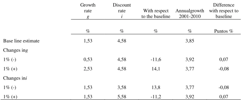
The JF estimation method relies on several important assumptions, including discount and growth rates necessary for estimating the human capital stock. This leads to ask some questions about the plausibility of the estimates, given that as shown in section 4.2., the human capital stock of Latin American countries exceeds several times the GDP. Table 3 assesses the behavior of human capital to changes in the growth and discount rates, using as example to Costa Rica in 2006. The analysis is performed by increasing and decreasing rates in a unit with regard to its initial value used in estimates of human capital, that is, 1.53% for the growth rate and 4.58% for the discount rate.

As can be seen, changes in the model parameters have an important impact on volumes of human capital stock nominal, a decline in the growth rate by one percentage point, all else being equal, reduces the stock of human capital by 11.6%, otherwise it increases by 14.1%. This same behavior is also observed to changes in the discount rate. In contrast, these changes produce very marginal changes in the rates of growth of volumes of the stock, whose differences from baseline are close to zero. This results have been found by national studies and by the consortium of the OECD (Gu and Wong, 2010); Liu, 2011; Christian, 2011; Wei, 2009).

Table 3: Sensitivity analysis for different growth and discount rates, Costa Rica in 2006

Growth rate

g

Discount rate

i

With respect to the baseline

Annualgrowth 2001-2010

Difference with respect to

baseline

% % % % Puntos %

Base line estimate 1,53 4,58 3,85

Changes ing

1% (-) 0,53 4,58 -11,6 3,92 0,07

1% (+) 2,53 4,58 14,1 3,77 -0,08

Changes ini

1% (-) 1,53 3,58 13,8 3,77 -0,08

1% (+) 1,53 5,58 -11,2 3,92 0,07

Note: estimates based on Equation 2 to changes in discount rates and growth.

4.3. Human Capital Index and education

P á g i n a 12 | 18

able to evaluate other population characteristics that affect the human capital index19_,

nonetheless, the necessary variables, for inclusion within it, differ substantially or are not available in the surveys of selected countries. Despite this, it can be used indirect techniques, such as econometric methods, to observe the effect of some of these variables on the estimated index. The idea would be to regress the index against some key variables that determining the human capital, but not explicitly included in the model, in order to analyze the behavior of education compared to these variables.

The selected variables are included on the criterion that the accumulation of human capital is done through investments that manifest in the form of formal and informal education, experience and health. In the literature is believed that schooling is the main component of this stock and can be measured by the average years of schooling. Informal education arises from the contexts in which individuals are developed, particularly the household background. The structure and resources allocated by households will impact significantly on performance both educational and labor, at later stages of individuals. To approximate this idea fertility rates are used, as these are associated with household sizes which in turn will determine the resources available for human capital formation (Rosenzweig et al., 1986; Rosenzweig et al. 2009; Temel, 2013). Labor experience is another important component of human capital formation. A proxy to this variable at international level is a complex issue. The difficulty is that the labors performed by individuals are not homogenous and labor insertion differs between countries, as well as the delay caused by increases in schooling, which an aggregate measure of this variable could be a very imperfect approximation of it. However, given its importance, in this study it was decided to measure it as the average age of the population minus 16, which was the age of reference for labor insertion in applying the prospective method, weighted by employment rates. Although data for construction of this variable are available in the data used in the household survey, employment rates require a longer horizon, given that for many of individuals the investments in experience took place long before the periods analyzed. Finally, another important factor in the formation of human capital is the health of individuals. The investments on this component have catalyst effects on productivity and academic performance of individuals.Nonetheless, the empirical literature has found a greater effect if these investments are done in early stages of human capital formation (Doyle et al., 2009). Thus, to approximate this dimension the mortality rate for children under five is used. It employ external data for the variables of fertility, employment rates and mortality rates from the World Bank.

Table 4 reports the results of the regressions for a panel data model with fixed effect20

that describe the determinants of human capital. Column 1 analyzes the effect of education on the index of human capital without controlling for other variables. This simple model confirms the results found in the prospective model, finding a positive and highly significant relationship between the education and the level of human capital. When entering a health variable, column 2, it shows that increases in infant mortality rates, reductions in health indicator, have a negative

19_{The method used in this document has segmented the population by age, gender and educational level, if}

information were available, more characteristics could be included to be evaluated in relative terms as determinants of human capital within the JF model. As mentioned, the method rests on the capacity of wages to capture most of the elements that are incorporated in human capital as the market pays for the complete package of qualities reflected in the marginal productivity of labor. In this sense, the method implicitly implies incorporating qualities like health or experience although it cannot express them explicitly by the information gap. Therefore, elements such as education, gender and age are absorbing the influence of these other elements, which could overstate their impact on human capital.

20_{Values of p-value less than 0.05 of the Breusch-Pagan and Hausman tests confirm the use of fixed effects in the}

P á g i n a 13 | 18

impact on human capital and different zero. Given the inclusion of this new variable, education remains highly significant but its impact is reduced substantially. In relative terms, this model shows health has a greater effect than that of education, the beta coefficients of both variables are 0.3 and -1.9 respectively21_{. Column 3 is added to the previous model the potential experience}

of workers. This new variable has no significant impact on the index of human capital22_.

Meanwhile the educational and health variables lose significance, and in the latter case it presents a significant reduction in the impact on the index.

In the next column the role of household investments in human capital determination is evaluated. This variable enters the model with a strong and highly significant impact, noting that the size of households, and therefore the resources for increases in human capital, are crucial for this stock. In this case education remains highly significant but its impact, measured by beta coefficient is relatively less to health and household size.

Table 4: Effects of key components on human capital

Dependent variable: Human Capital Index

(1) (2) (3) (4) (5)

Constant 2.736*** 6.148*** 2.690 5.641*** 2.601**

(0.501) (0.184) -2.254 (0.988) (0.957)

ln(Average years of schooling) 1.014*** 0.288*** 0.217** 0.214*** 0.115*

(0.251) (0.051) (0.077) (0.052) (0.053)

ln(Mortality rate) -0.662*** -0.440** -0.217* -0.156**

(0.045) (0.140) (0.102) (0.065)

ln(Experience) 1.011 0.115 -0.157

(0.662) (0.278) (0.266)

ln(Fertility) -1.074*** -0.503***

(0.206) (0.108)

ln(Population growth) 0.703***

(0.081)

Test F 16.39 147.47 138.09 187.98 632.63

Number of observations 95 95 95 95 95

Number of groups 10 10 10 10 10

R2_{within 0,206 0,519 0,531 0,582 0,611}

Note: robust errors in parentheses. Estimates are made based on a fixed effects model (FE) for an unbalanced panel. Statistical significance: *p<0.1, **p<0.05, ***p<0.01.

As was evidenced in section 4.3, much of human capital increases were the result of rises in population. In an effort to control this phenomenon results in column 5 added to the previous model the rate of population estimated at applying the model of JF. The results confirm the significant effect of the population growth in the indicator. Once the indicator is controlled by

21_{Table 5 reports the descriptive statistics of the variables used, including the standard deviations for the calculation}

of the beta coefficients, defined as the product between the coefficients estimated by its standard deviation and divided by the standard deviation of the dependent variable.

22_{This result contrasts with the results observed in regressions at the microeconomic level in which experience plays}

P á g i n a 14 | 18

population growth we have a closer view of the effect of education in relation to other determinants of human capital. The inclusion of population phenomena to model substantially reduces the effect of all the variables, keeping highly significant only household size (education and health do to values greater than 1%, while the experience is presented with the wrong sign and not significant). In relative terms, the results show that education has less impact (0.12) compared to health (-0.44) and household size (-0.65).

In summary, the results elucidates the importance of education as a determinant in the formation of human capital. However, they also note that other investments, such as health and family contexts, play a no less to the education role. This is very important because in related literature generally tends to reduce human capital toward a unidimensional approach based on education. This practice depart from the assumption that education is fundamental to human capital, as is evidenced in this document, but is wrong to point implicitly that this component should include the largest percentage the behavior of this stock and therefore enough with an educational variable to characterize it. Conversely,the results of this section show that the formation of this stock is also significantly influenced by investments different to made in education.

It should be noted some shortcomings of the estimates. A more efficient way to assess the relative importance of education in the current context would be to include other determinants of human capital in the model of JF. This is possible at national level to some countries, howevergiven the limitations international data prevent this possibility. Second, the estimates may be biased, particularly by endogeneity problems. Indeed, the method of JF rests on wage earnings, which in the short term are affected by the economic cycle and, in the long-term by trends in economic growth. Then, human capital may affect the levels of education, fertility and health. This simultaneity problem can create a problem of endogeneity in the model. The solution has been the use of instrumental variables. However, achieving strong and valid instruments is a recent discussion in econometrics (Aghion and Durlauf, 2005). More recently the use of dynamic panel techniques have been more convenient for these problems (Arellano and Bond, 1991; Arellano and Bover, 1995; Blundell and Bond, 1998.) However, the small number of countries and periods makes it not advisable to use this technique in the current document. Finally, it would be interesting to do the same analysis for some more developed countries. Nonetheless, estimated by Liu (2011) series are not reported.

5. Conclusions

The first important fact of this study is that although the dimensions of the stock of human capital for Latin American countries are large (on average, the ratio is almost five times relative to GDP and two in reference to physical capital) they become modest when it is compared to those of the OECD countries. The evidence presented is in line with the classical theory of economic growth which it is stated that countries with higher levels of per capita income exhibit higher CH/GDP ratios because they would have lower average capital productivities as well as a better use of the positive externalities of capital Human, among others.

P á g i n a 15 | 18

able to compensate for the negative effects of population aging. However, due to the own dynamics of educational attainment, this compensatory effect tends to run out over time. For developed countries, levels in terms of educational attainment have reached such a point that it will be difficult to experience significant increases in this indicator given the expected returns to compensate for marginal increases in schooling. In the meantime, although developing countries grow at higher rates, their long term trend seems to approximate those more developed. In this way, increases in human capital via educational attainment seem doomed to be depleted in the long run.

P á g i n a 16 | 18

References

Ahlroth, S., Bjorklund, A. and Forslund, A. (1997). The output of the Swedish education sector. Review of Income and Wealth, 43 (1), 89-104.

Arellano, M., and S. Bond. 1991. Some tests of specification for panel data: Monte Carlo evidence and an application to employment equations. Review of Economic Studies 58: 277– 297.

Arellano, M., and O. Bover. 1995. Another look at the instrumental variable estimation of error-components models. Journal of Econometrics 68: 29–51.

Barro, R. and Lee, J. (2013). A new data set of educational attainment in the world, 1950–2010. Journal of Development Economics, 104: 184-198.

Becker, G. (1964), Human Capital. Columbia UP, New York.

Blundell, R., and S. Bond. 1998. Initial conditions and moment restrictions in dynamic panel data models. Journal of Econometrics 87: 115–143.

Christian, M. (2011). Human Capital Accounting in the United States: Context, Measurement, and Application. Wisconsin Center for Education Research, July 2011.

Coremberg, A. (2010). The Economic Value of Human Capital and Education in an Unstable Economy: Argentina. Paper Prepared for the 31st General Conference of The International Association for Research in Income and Wealth.

Diewert, W. Erwin (1976), "Exact and Superlative Index Numbers", Journal of Econometrics 4: 115-145.

Doyle, O., Harmon, C., Heckman, J. and Tremblay, R. (2009). Investing in early human development: Timing and economic efficiency. Economics and Human Biology, vol.7(1): 1-6.

Durlauf, S., Johnson, P. A. y Temple, J. (2005). Growth econometrics. In P. Aghion, y S. Durlauf (Eds). Handbook of economic growth. Amsterdam: North Holland.

Ervik, A., E. Holmoy, y T. Haegeland (2003), "A Theory-Based Measure of the Output of the Education Sector," Discussion Papers No. 353, Statistics Norway.

Folloni, G. y Vittadini, G. (2009). Human capital measurement: A Survey. Journal of EconomicSurveys, Vol. 24, No. 2, pp. 248-279.

P á g i n a 17 | 18

Gasparini, L., M., Marchionni y W. Sosa (2000). La distribución del ingreso en Argentina y en la Provincia de Buenos Aires. Cuadernos de Economía No. 49. Ministerio de Economía de la Provincia de Buenos Aires, República de Argentina.

Gu, W. and A. Wong (2008), Human Development and its Contribution to the Wealth Accounts in Canada. Paper for workshop on the measurement of human capital, Turin, November 2008. MicroEconomic Analysis Division, Statistics Canada, October 2008.

Gu, W. and A. Wong (2010), Estimates of Human Capital in Canada: The Lifetime Income Approach. Economic Analysis Research Paper Series 11F0027M No.062, Economic Analysis Division, Statistics Canada, Ottawa.

Guerriero, M. (2012). The Labour Share of Income around the World. Evidence from a Panel Dataset. Institute for Development Policy and Management (IDPM). Development Economics and Public Policy, Working Paper Series WP No. 32.

Jones, R. and V. Fender (2011), Human Capital Estimates – 2010. Office of National Statistics, UK.

Jones, R. y B. Chiripanhura (2010), "Measuring the U.K.'s Human Capital Stock," Economic and Labour Market Review 4(11), pp. 36-63.

Jorgenson, D.W. y Fraumeni, B. M. (1989). The accumulation of human and non-human capital,1948-1984. In Lipsey, R. E. and Tice, H. S., editors, The Measurement of Savings, Investment andWealth, pages 227–282. The University of Chicago Press, Chicago, I.L.

Jorgenson, D.W. and B.M. Fraumeni (1992), The output of the education sector. In: Z. Griliches (ed.), Output measurement in the services sector, University of Chicago Press, pp.303-338. USA.

Le, T., J. Gibson and L. Oxley (2003), Cost- and income-based measures of human capital. Journal of Economic Surveys 17:3, pp.271-307. NewZealand.

Li, H., Y. Liang, B.M. Fraumeni, Z. Liu and X. Wang (2012), Human Capital in China, 1985-2008. Unpublished, Central University of Finance and Economics, Beijing, China.

Liu, G. (2011), Measuring the stock of human capital for comparative analysis: An application of the lifetime income approach to selected countries. OECD Statistics Directorate Working Paper 41, STD/DOC (2011)06, OECD, Paris.

Liu, G. and M. Greaker (2009), Measuring the stock of human capital for Norway: A lifetime labour income approach. Working Paper 10 for ECE Conference of European Statisticians, Geneva, 23-24 September 2009. Working Paper 2009/12, Statistics Norway.

P á g i n a 18 | 18

Lucas, Robert E. Jr (1990), "Why doesn't Capital Flow from Rich to Poor Countries?", American Economic Review 80: 92–96

Mincer, J. (1974), Schooling, Experience, and Earnings. Columbia University Press, New York.

Piketty, T., 2014. Capital in the 21st Century. Harvard University Press, Cambridge, MA

Temel, T. (2013). Family size, Human Capital and Economic Growth: Structural Path Analysisof Rwanda. Journal of Economic Development, vol. 38(4): 39-73.

Wei, H. (2004), Measuring the Stock of Human Capital for Australia, Working Paper No. 2004/1, Australian Bureau of Statistics, Sydney, February 2004.

Wei, H. (2008), Measuring Human Capital Flows for Australia: A Lifetime Labour Income Approach. ABS Research Paper no. 1351.0.55.023. Australian Bureau of Statistics, Sydney.

Wei, H. (2009), Developments in the estimation of the value of human capital for Australia. Paper for ECE Conference for European Statisticians, Geneva, 23-24 September 2009. Australian Bureau of Statistics, Sydney.

Schultz, T.W. (1961) Investment in human capital. American Economic Review 51(1):1–17.

Rensman, M. (2013). Human capital in the Netherlands. Statistics Netherlands. Discussion Paper.

Rosenzweig, M. (1986). Birth Spacing and Sibbling Inequality: Asymetric Information within the Family. International Economic Review, Vol. 27(1): 55-76.

Rosenzweig, M. and Zhang, J. (2009). Do Population Control Policies Induce more Human capital Investment? Twins, Birth weigth and China's “One-Child” Policy. Review of Economics Studies, Oxford University Press, vol. 76(3): 1149-1174.

OECD (1998) –“Human Capital” investment: an international comparison, Paris.