On the population median estimation using quartile double ranked set sampling

Amer Ibrahim Al-Omari

Faculty of Science, Department of Mathematics Al al-Bayt University, Mafraq, Jordan

[email protected] Loai M. Al-Zubi

Faculty of Science, Department of Mathematics Al al-Bayt University, Mafraq, Jordan

Ahmad Khazaleh

Faculty of Science, Department of Mathematics Al al-Bayt University, Mafraq, Jordan

Abstract

In this article, quartile double ranked set sampling (QDRSS) method is considered for estimating the population median. The sample median based on QDRSS is suggested as an estimator of the population median. The QDRSS is compared with the simple random sampling (SRS), ranked set sampling (RSS) and quartile ranked set sampling (QRSS) methods for estimating the population median. To verify this method a real data example is applied. It turns out that for the symmetric distributions considered in this study, the QDRSS estimators are unbiased estimators of the population median and are larger than their counterparts using SRS, RSS and QRSS based on the same sample size of measured units. For asymmetric distributions, QDRSS is biased. It is more efficient than the SRS and the QRSS for all samples of size m while it is more efficient than RSS if m4.

Keywords: Simple random sampling; Quartile ranked set sampling; Ranked set sampling; Quartile double ranked set sampling; Median.

1. Introduction

Ranked set sampling was first suggested by McIntyre (1952) as a cost efficient sampling procedure when compared to the commonly used simple random sampling in situations where visual ordering of set units can be done easily, but the exact measurement of the units is difficult and expensive. McIntyre (1952) found that the RSS is more efficient than SRS for estimating the population mean.

Let X be a random variable with a probability density function (pdf) f x( ), and a cumulative distribution function (cdf) F x( ) with mean



and variance 2. Also, let f( : )i m ( )x be the pdf

of the ith order statistic of a random sample of size m, Xi1,Xi2,...,X for im i1, 2,...,m.

Then, the pdf of X( : )i m is given by





( ) 1 ( : ) 0 1 ( ) 1 ( ) ( , 1) F x m i i i m d f x u u f x B i m i dx      



,

where 1 1 1 0 ( , ) (1 ) , 0, 0 B

 





u u  du







 , with mean



_{( : )i m} xf_{( : )i m} ( )x dx   



and variance



( : )2i m



x



( : )i m



2 f( : )i m ( )x dx  





 , David and Nagaraja (2003).

Takahasi and Wakimoto (1968) provided the necessary mathematical theory of RSS. They showed that ( : ) 1 1 ( ) ( ) m i m i f x f x m  



, ( : ) 1 1 m i m i m    



and 2 ( : )2



( : )



2 1 1 1 m 1 m i m i m i i m m









  







 .

Muttlak (1997) suggested median ranked set sampling for estimating the population mean. Al-Saleh and Al-Kadiri (2000) considered double ranked set sampling (DRSS) method for estimating the population mean, and they showed that the ranking at the second stage is easier than the ranking at the first stage.

The double ranked set sampling method can be described as follows: Randomly identify m 3

units from the target population and divide them randomly into m sets each of size m2. The procedure of ranked set sampling is applied to these sets to obtain m ranked set samples each of size m, again reapply the ranked set sampling procedure on the m ranked set samples to obtain a DRSS of size m.

Al-Saleh and Al-Omari (2002) generalized the DRSS to multistage ranked set sampling to increase the efficiency of the estimators for specific value of the sample size. Muttlak (2003) proposed quartile ranked set sampling (QRSS) for estimating the population mean. Al-Omari and Al-Saleh (2009) suggested quartile double ranked set sampling (QDRSS) for estimating the population mean. Al-Omari (2010) suggested an estimator of the population median using double robust extreme ranked set sampling. Entropy estimation and goodness-of-fit tests for the inverse Gaussian and Laplace distributions using paired ranked set sampling method is suggested by Al-Omari and Haq (2015). Biradar and Santosha (2015) proposed estimation of the population mean using paired ranked set sampling. Santos and Barrios (2015) considered predictive accuracy of logistic regression model using ranked set samples. Confidence intervals and hypothesis tests for a population mean using ranked set sampling are considered by Stella et al. (2015). For more about RSS and its modifications see Sinha et al. (2006), Ozturk and Jozani (2014), Hatefi et al. (2014), Samawi and Al-Saleh (2014), Bouza (2002), and Tiwari and Pandey (2013).

2. Estimation of the population median 2.1. Using SRS

Let X1,X2,...,X be a random sample of size m from a distribution with pdf m f x , cdf ( )

( )

F x , mean



, median



and variance 2

.

The SRS estimator of the population median from a sample of size m at the hth cycle

1 2 2 2 2 , if is odd ˆ 1 , if is even. 2 m h SRS m m h h X m X X m                             _  _     (1)

Based on f( : )i m ( )x if m is odd, the pdf of 1 2 m X_{ }     is given by





21 1 2 2 ! ( ) ( ) 1 ( ) ( ) 1 ! 2 m m m f x F x F x f x m          _  _      _{ }   , (2) and if m is even



 

2



2 2 2 ! ( ) ( ) 1 ( ) ( ) 2 ! ! 2 2 m m m m f x F x F x f x m m                       , (3) and



 



2 2 2 2 2 ! ( ) ( ) 1 ( ) ( ) 2 ! ! 2 2 m m m m f x F x F x f x m m                        . (4) 2.2. Using RSS

The RSS (McIntyre, 1952) involves randomly selecting m units from the population. 2

These units are randomly allocated into m sets, each of size m. The m units of each sample are ranked visually or by any inexpensive method with respect to a variable of interest. From the first set of m units, the smallest ranked unit is measured. From the second set of m units, the second smallest ranked unit is measured. The process is continued until from the

mth set of m units the largest ranked unit is measured. The process can be repeated n times

to get a sample of size mn from the initial m2n units.

Let X_11h,X_12h,...,X_1mh; X_21h,X_22h,...,X_2mh; …; X_{m h1} ,X_{m h2} ,...,X_mmh be m independent simple random samples each of size m in the hth cycle



h1, 2,...,n



. Let Xi(1)h, Xi(2)h,

…,X_{i m h( )} be the order statistics of the ith sample X_{i h1} ,X_{i h2} ,...,X_imh for i1, 2,..., m . Therefore, X1(1)h,X2(2)h,…,Xm m h( ) denote the measured RSS units.

The RSS estimator of the population median  from a sample of size m at the hth cycle



h1, 2,...,n



is given by



1(1) 2(2) ( )



ˆ_RSS Median X _h,X _h,...,X_{m m h}



 . (5)

2.3. Using QRSS

The QRSS procedure, suggested by Muttlak (2003) is described as follows: select m random samples each of size m units from the target population and rank the units within each sample with respect to the variable of interest. If the sample size is even, select for measurement from the first m/ 2 samples the q m1( 1)th smallest ranked unit and from the

second m/ 2 samples the q m3( 1)th smallest ranked unit, where q10.25 and q3 0.75,

where the nearest integers of q m1( 1)th and q m3( 1)th will always be taken. If the

sample size is odd, select from the first (m1) / 2 samples the q m1( 1)th smallest ranked

unit and from the other (m1) / 2 samples the q m3( 1)th smallest ranked unit, and from

one sample the median of that sample for actual measurement. The procedure can be repeated n times if needed to increase the sample size to nm units.

If the sample size is even, at the hth cycle



h1, 2,...,n



, let

1

* ( ( 1)) i q m h

X _ be the first quartile of the ith sample 1, 2,...,

2 m i  _     , and 3 * ( ( 1)) i q m h

X _ be the third quartile of the ith sample

2 4 , ,..., 2 2 m m i   m  _   

 . Therefore, the measured QRSSE units are 1

* 1(q m( 1))h,..., X _ 1 * ( ( 1)) 2 m q m h X  , 3 * 2 ( ( 1)) 2 m q m h X _  ,..., 3 * ( ( 1)) m q m h

X _ . The QRSSE estimator of the population median is given by 1 3 1 3 * * * * * 1( ( 1)) 2 ( ( 1)) ( ( 1)) ( ( 1)) 2 2 ˆ_QRSSE Median _{q m h},..., _m , _m ,..., _{m q m h} q m h q m h X X X X



_{  }      _{ }  , (6)

If the sample size m is odd, let

1

* ( ( 1)) i q m

X _ be the first quartile of the ith sample 1 1, 2,..., 2 m i   _     , * 1 2 m i h X_{ }    

be the median of the ith sample of the rank 1

2 m i  , and let 3 * ( ( 1)) i q m h

X _ be the third quartile of the ith sample 3, 5,...,

2 2 m m i   m  _     . Therefore, the

measured QDRSSO units are

1 * 1(q m( 1))h, X _ ..., 1 * 1 ( ( 1)) 2 , m q m h X _  * 1 1 2 2 m m h X _{ }     , 3 * 3 ( ( 1)) 2 , m q m h X _  ..., 3 * ( ( 1)) m q m h

X _ . The estimator of the population median using QRSSO is defined as

1 3 1 3 * * * * * * 1( ( 1)) 1 1 1 3 ( ( 1)) ( ( 1)) ( ( 1)) 2 2 2 2 ˆ_QRSSO Median _{q m h},..., _m , _{m m} , _m ,..., _{m q m h} q m h h q m h X X X X X



_{     }  _{ }         _{ }     (7) 2.4 . Using QDRSS

The quartile double ranked set sampling method (Al-Omari and Al-Saleh, 2009) can be carried out as follows:

Step 1: Randomly select m units from the target population and allocate them into 3 m sets each of size m units. 2

Step 2: Rank the units within each set with respect to the variable of interest, and then apply

the RSS method on the m sets. This step yields m ranked set samples each of size m.

Step 3: Without doing any actual quantifications, apply the QRSS method on the m DRSS

a sample of size mn from the QDRSS data. For even and odd sample sizes we denote the measured QDRSS units as QDRSSE and QDRSSO, respectively.

Let us consider the following example. Select a random sample of size m8, so we will select m3512 units. Allocate them into 8 sets each of 64 units. Rank the units within each set with respect to the variable of interest. Let Xjik be the ith unit



i1, 2,...,8



in the jth

set



j1, 2,...,8



in the kth subset



k 1, 2,...,8



. Select the Xj i k( ) from each subset, the

processes appears as shown below:

















1(1)1 1(2)1 1(7)1 1(8)1 1(1)2 1(2)2 1(7)2 1(8)2 1(1)8 1(2)8 1(7)8 1(8)8 1(1)1 1(2)1 1(7)1 1(8)1 The 1st set of size 64 units

, ,..., , , ,..., , , ,..., , , ,..., , X X X X X X X X X X X X X X X X                     ,…,

















8(1)1 8(2)1 8(7)1 8(8)1 8(1)2 8(2)2 8(7)2 8(8)2 8(1)7 8(2)7 8(7)7 8(8)7 8(1)8 8(2)8 8(7)8 8(8)8 The 8th set of size 64 units

, ,..., , , ,..., , , ,..., , , ,..., , X X X X X X X X X X X X X X X X                    

Select the ith smallest ranked unit from the ith subset



i1, 2,..,8



in each set. This step yields 64 units, i.e., 8 RSS sets each of size 8 as follows:



 

 

 

 

 

 

 





X1(1)1 , X1(2)2 , X1(3)3 , X1(4)4 , X1(5)5 , X1(6)6 , X1(7)7 , X1(8)8



,



 

 

 

 

 

 

 





X2(1)1 , X2(2)2 , X2(3)3 , X2(4)4 , X2(5)5 , X2(6)6 , X2(7)7 , X2(8)8



,



 

 

 

 

 

 

 





X3(1)1 , X3(2)2 , X3(3)3 , X3(4)4 , X3(5)5 , X3(6)6 , X3(7)7 , X3(8)8



,



 

 

 

 

 

 

 





X4(1)1 , X4(2)2 , X4(3)3 , X4(4)4 , X4(5)5 , X4(6)6 , X4(7)7 , X4(8)8



,



 

 

 

 

 

 

 





X5(1)1 , X5(2)2 , X5(3)3 , X5(4)4 , X5(5)5 , X5(6)6 , X5(7)7 , X5(8)8



,



 

 

 

 

 

 

 





X6(1)1 , X6(2)2 , X6(3)3 , X6(4)4 , X6(5)5 , X6(6)6 , X6(7)7 , X6(8)8



,



 

 

 

 

 

 

 





X7(1)1 , X7(2)2 , X7(3)3 , X7(4)4 , X7(5)5 , X7(6)6 , X7(7)7 , X7(8)8



,



 

 

 

 

 

 

 





X8(1)1 , X8(2)2 , X8(3)3 , X8(4)4 , X8(5)5 , X8(6)6 , X8(7)7 , X8(8)8



.

Without doing any actual quantifications on these sets, rank the units within each set with respect to the variable of interest and then select the first quartile Xi(2)1



from the ith set (i1, 2,3, 4) and select the third quartile Xi(7)1



from the ith set (i5, 6, 7,8) as shown below:



 

 

 

 

 

 

 





X1(1)1 , X1(2)1 , X1(3)1 , X1(4)1 , X1(5)1 , X1(6)1 , X1(7)1 , X1(8)1



        ,



 

 

 

 

 

 

 





X1(1)2 , X1(2)2 , X1(3)2 , X1(4)2 , X1(5)2 , X1(6)2 , X1(7)2 , X1(8)2



        ,



 

 

 

 

 

 

 





X1(1)3 , X1(2)3 , X1(3)3 , X1(4)3 , X1(5)3 , X1(6)3 , X1(7)3 , X1(8)3



        ,



 

 

 

 

 

 

 





X1(1)4 , X1(2)4 , X1(3)4 , X1(4)4 , X1(5)4 , X1(6)4 , X1(7)4 , X1(8)4



        ,



 

 

 

 

 

 

 





X1(1)5 , X1(2)5 , X1(3)5 , X1(4)5 , X1(5)5 , X1(6)5 , X1(7)5 , X1(8)5



        ,



 

 

 

 

 

 

 





X1(1)6 , X1(2)6 , X1(3)6 , X1(4)6 , X1(5)6 , X1(6)6 , X1(7)6 , X1(8)6



        ,



 

 

 

 

 

 

 





X1(1)7 , X1(2)7 , X1(3)7 , X1(4)7 , X1(5)7 , X1(6)7 , X1(7)7 , X1(8)7



        ,



 

 

 

 

 

 

 





X1(1)8 , X1(2)8 , X1(3)8 , X1(4)8 , X1(5)8 , X1(6)8 , X1(7)8 , X1(8)8



        .

This process produces



1(2)1, 1(2)2, 1(2)3, 1(2)4, 1(7)5, 1(7)6, 1(7)7, 1(7)8



v

X X X X X X X X as a QDRSSE

of size 8. The median of these units can be considered as an estimator of the population median. It is defined as



1(2)1 1(2)2 1(2)3 1(2)4 1(7)5 1(7)6 1(7)7 1(7)8



ˆ_QDRSSE Median X ,X ,X ,X ,X ,X ,X ,X



 _        

. (8) The most interesting thing here is that the number of quantified units using QDRSS is 8 which will be compared with a SRS of size 8 is a small relative to to the number of sampled units 512. Hence, the information contained in the QDRSS sample is more than the information in the 8 units of the SRS.

In the hth cycle



h1, 2,...,n



if the sample size is even, let

1

( ( 1)) i q m h

X _ be the first quartile of the ith sample 1, 2,...,

2 m i  _     , and Xi q m(3( 1))h 

 be the third quartile of the ith sample

2 4 , ,..., 2 2 m m i   m  _   

 . Hence, the measured QDRSSE units are X1(q m1( 1))h,...,

  1 ( ( 1)) 2 m q m h X  , 3 2 ( ( 1)) 2 m q m h X_  ,..., Xm q m( 3( 1))h 

 . The suggested QDRSSE estimator of the

population median is given by

1 3 1 3 1( ( 1)) 2 ( ( 1)) ( ( 1)) ( ( 1)) 2 2 ˆQDRSSE Median q m h,..., m , m ,..., m q m h q m h q m h X X X X



      _  _     _{ }  , (9)

If the sample size m is odd, let Xi q m(₁( 1))



 be the first quartile of the ith sample

1 1, 2,..., 2 m i   _     , and 1 2 m i h X_{  }    

be the median of the ith sample of the rank 1

2 m i  , and 3 ( ( 1)) i q m h

X _ be the third quartile of the ith sample 3, 5,...,

2 2 m m i   m  _     . Therefore, the

QDRSSO measured units are

1 1 1( ( 1)) 1 ( ( 1)) 2 ,..., , q m h m q m h X _ X_  1 1 2 2 m m h X_{  }     , 3 3 ( ( 1)) 2 , m q m h X_  3 ( ( 1))

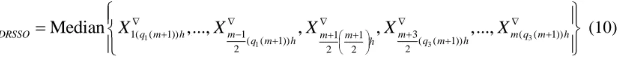
...,X_{m q m} _{ h}. The suggested estimator of the population median using QDRSSO is defined as

1 3 1 3 1( ( 1)) 1 1 1 3 ( ( 1)) ( ( 1)) ( ( 1)) 2 2 2 2 ˆ_QDRSSO Median _{q m h},..., _m , _{m m} , _m ,..., _{m q m h} q m h h q m h X X X X X         _     _           _{ }     (10) 4. Simulation Study

In this section, a simulation study is considered to compare the proposed estimators for the population median using QDRSS, QRSS, RSS relative to SRS. Six probability distribution functions were considered for the populations: Uniform, Normal, Logistic, Exponential, Gamma and Weibull. 60,000 samples were generated and the averages of these samples were compared.

If the distribution is symmetric the efficiency of RSS, QRSS and QDRSS relative to SRS, is defined as, respectively,



ˆ ,ˆ



Var





ˆ





ˆ Var SRS RSS SRS RSS eff









 ,











ˆ



Var ˆ ,ˆ ˆ Var SRS QRSS SRS QRSS eff









 , and





Var





ˆ





ˆ ,ˆ ˆ Var SRS QDRSS SRS QDRSS eff









   .

If the distribution is asymmetric, the efficiency is defined by













ˆ MSE ˆ ,ˆ ˆ MSE SRS RSS SRS RSS eff









 ,











ˆ



MSE ˆ ,ˆ ˆ MSE SRS QRSS SRS QRSS eff









 , and











ˆ



MSE ˆ ,ˆ ˆ MSE SRS QDRSS SRS QDRSS eff









 

 , where MSE

 

 Var

 

 _E

 

 



_2. Results of simulation in terms of the efficiency and bias values for RSS, QRSS and DQRSS are summarized for m4,5 in Table 1, for m6, 7 in Table 2, for m10,11 in Table 3 and for m12 in Table 4.

Table 1: The efficiency and bias values of RSS, QRSS, and QDRSS with respect to SRS in estimating the population mean with m4 and 5.

Distribution m4 m5 RSS QRSS QDRSS RSS QRSS QDRSS Uniform (0,1) Eff 1.988 2.400 4.517 1.885 2.358 3.696 Normal (0,1) Eff 2.206 1.979 3.016 2.101 2.680 4.440 Logistic (-1,1) Eff 2.268 1.872 2.631 2.177 2.813 4.713 Exponential (1) Eff 2.299 1.313 1.347 2.296 3.049 5.105 Bias 0.094 0.218 0.268 0.043 0.034 0.021 Gamma (1,2) Eff 2.314 1.311 1.381 2.319 3.058 5.025 Bias 0.192 0.437 0.531 0.080 0.065 0.039 Weibull (1,3) Eff 2.275 1.271 1.369 2.281 3.054 5.187 Bias 0.029 0.662 0.804 0.127 0.105 0.061

Table 2: The efficiency and bias values of RSS, QRSS, and QDRSS with respect to SRS in estimating the population mean with m6 _{and 7.}

Distribution m6 m7 RSS QRSS QDRSS RSS QRSS QDRSS Uniform (0,1) Eff 2.382 2.816 6.111 2.226 2.041 2.886 Normal (0,1) Eff 2.750 3.106 6.568 2.522 2.351 3.334 Logistic (-1,1) Eff 2.756 3.190 6.682 2.551 2.368 3.397 Exponential (1) Eff 2.945 3.114 5.850 2.670 2.437 3.674 Bias 0.048 0.056 0.064 0.026 0.027 0.019 Gamma (1,2) Eff 2.857 3.183 5.851 2.700 2.480 3.708 Bias 0.098 0.110 0.130 0.054 0.062 0.042 Weibull (1,3) Eff 2.877 3.159 5.764 2.647 2.501 3.637 Bias 0.149 0.165 0.198 0.080 0.083 0.062

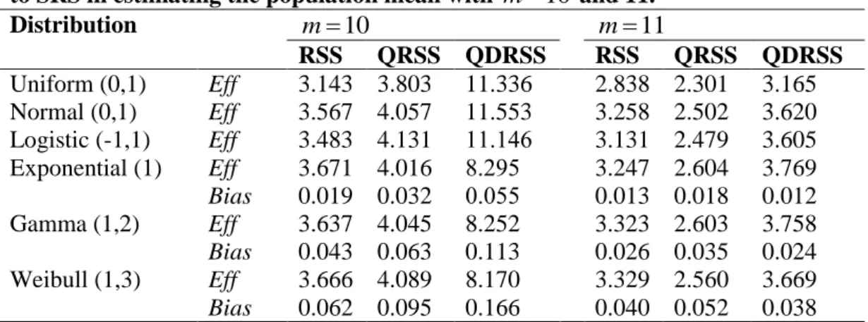
Table 3: The efficiency and bias values of RSS, QRSS, and QDRSS with respect to SRS in estimating the population mean with m10 _{and 11.}

Distribution m10 m11 RSS QRSS QDRSS RSS QRSS QDRSS Uniform (0,1) Eff 3.143 3.803 11.336 2.838 2.301 3.165 Normal (0,1) Eff 3.567 4.057 11.553 3.258 2.502 3.620 Logistic (-1,1) Eff 3.483 4.131 ..1.11 3.131 2.479 3.605 Exponential (1) Eff 3.671 4.016 512.8 3.247 2.604 3.769 Bias 0.019 0.032 01088 0.013 0.018 0.012 Gamma (1,2) Eff 3.637 4.045 8.252 3.323 2.603 3.758 Bias 0.043 0.063 0.113 0.026 0.035 0.024 Weibull (1,3) Eff 3.666 4.089 8.170 3.329 2.560 3.669 Bias 0.062 0.095 0.166 0.040 0.052 0.038

Table 4: The efficiency and bias values of RSS, QRSS, and QDRSS with respect to SRS in estimating the population mean with respect to SRS with m12.

Distribution RSS QRSS QDRSSE Uniform (0,1) Eff 3.464 4.067 14.298 Normal (0,1) Eff 3.953 4.139 12.492 Logistic (-1,1) Eff 3.833 4.080 11.863 Exponential (1) Eff 3.914 3.647 5.021 Bias 0.017 0.047 0.094 Gamma (1,2) Eff 3.997 3.697 4.985 Bias 0.032 0.093 0.188 Weibull (1,3) Eff 3.989 3.654 5.119 Bias 0.044 0.140 0.283

According to these results, we conclude:

1) If the underlying distribution is symmetric about its mean, then a)



ˆQDRSSE



and



ˆQDRSSO



are unbiased estimators of the population median with smaller variance than the ˆSRS estimator based on the same sample size. As an example, for

7

m , the efficiency of



ˆ_QDRSSO is 3.334 for estimating the population median of the standard normal distribution.

b)



ˆQDRSSE



and



ˆQDRSSO



are more efficient than ˆ_RSS. For example, when m11 the efficiency of



ˆ_QDRSSO and ˆ_RSS are 3.165 and 2.838, respectively, for estimating the population median of the standard uniform distribution.

c)



ˆQDRSSE



and



ˆQDRSSO



are more efficient than ˆQRSS. For m10, the efficiency

values of



ˆQDRSSE



and ˆQRSS are 11.146 and 4.131, respectively for estimating the

median of the Logistic distribution with parameters -1 and 1. 2) If the underlying distribution is asymmetric, we noted that a)



ˆQDRSSE



and



ˆQDRSSO



have a small bias. As an example, for m12 the efficiency of

ˆQDRSSE





is 5.021 with bias 0.094 for estimating the median of the exponential distribution with parameter 1.

b)



ˆ_QDRSSE and



ˆ_QDRSSO are more efficient than ˆ_RSS if m4 and they are more efficient than ˆQRSS for all cases considered in this study based on the same number

of measured units. For example, with m10 the efficiency values of ˆ_RSS, ˆ_QRSS and



ˆ_QDRSSE are, respectively, 3.666, 4.089 and 8.170 for estimating the median of Weibull distribution with parameters 1 and 3.

3) Comparing



ˆQDRSSE



to



ˆQDRSSO



, it is found that



ˆQDRSSE



is more efficient. For example, for m6 and 7, the efficiency of



ˆQDRSSE



and



ˆQDRSSO



are, respectively, 6.568 and 3.334 for estimating the median of standard normal distribution. This may be due to that: in the case of odd sample size we select only the median of the set of

the rank 1

2

m

i  , while with even sample size we identify the first or the third quartile of the ith sample.

5. Real Data Application

In this section, to evaluate the performance of QDRSS in estimating the population median of a real data, a study is conducted to estimate the median weight of 342 students. Balanced ranked set sampling is considered and all samples were done without replacement.

Let i for i1, 2,...,342 be the weight of the ith student in the population. The

mean , median  and the variance



2 of the population are, respectively

342 1 1 50.047 kg 342 i i Z



 



 ,



Median



Z i_i, 1, 2,...,342



171 172 48 2 Z Z   , and 342 2 2 2 1 1 ( ) 258.93kg 342 i i Z





 



  .

The skewness of the 342 observations is 1.244, which means that these data are asymmetrically distributed, and so the QDRSS estimators will be biased. Hence, the bias

and mean squared error (MSE) of the estimators were computed. The efficiency of RSS, QRSS and QDRSS with respect to SRS are obtained using Equations (8), (9), and (10). The simulated median, bias, MSE and the efficiency values are summarized in Table 5.

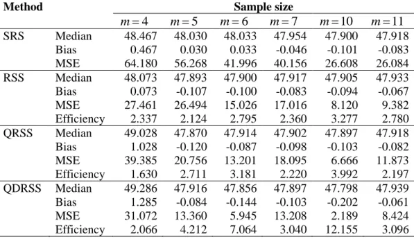
Table 5: The efficiency and bias values of RSS, QRSS and QDRSS relative to SRS with sample size m4,5, 6, 7,10,11 for estimating the median weight of 342 students.

Method Sample size

4 m m5 m6 m7 m10 m11 SRS Median 48.467 48.030 48.033 47.954 47.900 47.918 Bias 0.467 0.030 0.033 -0.046 -0.101 -0.083 MSE 64.180 56.268 41.996 40.156 26.608 26.084 RSS Median 48.073 47.893 47.900 47.917 47.905 47.933 Bias 0.073 -0.107 -0.100 -0.083 -0.094 -0.067 MSE 27.461 26.494 15.026 17.016 8.120 9.382 Efficiency 2.337 2.124 2.795 2.360 3.277 2.780 QRSS Median 49.028 47.870 47.914 47.902 47.897 47.918 Bias 1.028 -0.120 -0.087 -0.098 -0.103 -0.082 MSE 39.385 20.756 13.201 18.095 6.666 11.873 Efficiency 1.630 2.711 3.181 2.220 3.992 2.197 QDRSS Median 49.286 47.916 47.856 47.897 47.798 47.939 Bias 1.285 -0.084 -0.144 -0.103 -0.202 -0.061 MSE 31.072 13.360 5.945 13.208 2.189 8.424 Efficiency 2.066 4.212 7.064 3.040 12.155 3.096

Table 5 shows that there is a small difference between the true and the estimated median. This difference is due to skewness of the data used in this example. For m4, RSS is more efficient than QDRSS. While, QDRSS is more efficient than RSS. In addition, it can be noted that QDRSS is more efficient than QRSS for all sample sizes considered in Table 5. Furthermore, the results of real data example are agreed with the results of the simulation study conducted in Section 4.

6. Conclusion

In estimating the population median, a good achievement is gained in efficiency using QDRSS, QRSS, RSS regardless the underlying distribution whether it is symmetric or asymmetric. QDRSS estimators are unbiased estimators of the population median when distributions are symmetric. In addition, it is found that QDRSS is more efficient than RSS if m4 and more efficient than QRSS in all cases considered in this study. However, the QDRSS is recommended for estimating the population median of symmetric distributions.

Acknowledgement

The authors are thankful to the reviewer and the associate editor for valuable comments that significantly improved the current version of the article.

References

1. Al-Omari, A.I. (2010). Estimation of the population median of symmetric and asymmetric distributions using double robust extreme ranked set sampling. Revista

Investigación Operacional, 31(3): 199-207.

2. Al-Omari, A.I. and Haq, A. (2015). Entropy estimation and goodness-of-fit tests for the inverse Gaussian and Laplace distributions using paired ranked set sampling.

Journal of Statistical Computation and Simulation, accepted, DOI:10.1080/00949

655.2015. 1109097.

3. Al-Omari, A.I. and Jaber, K. (2008). Percentile double ranked set sampling. Journal of

Mathematics and Statistics, 4(1): 60-64.

4. Al-Saleh, M.F. and Al-Kadiri, M.A. (2000). Double ranked set sampling. Statistics

and Probability Letters, 48(2): 205-212.

5. Al-Saleh, M.F. and Al-Omari, A.I. (2002). Multistage ranked set sampling. Journal of

Statistical Planning and Inference, 102(2): 273-286.

6. Al-Omari, A.I. and Al-Saleh, M.F. (200.). Quartile double rankled set sampling for estimating the population mean. Economic Quality Control, 24(2): 243 – 253.

7. Balakrishnan, N. and Li, T. (2006). Confidence intervals for quantiles and tolerance intervals based on ordered ranked set samples. Annals of the Institute of Statistical

Mathematics, 58: 757-777.

8. Biradar, B.S. and Santosha, C.D. (2015). Estimation of the population mean using paired ranked set sampling. Open Journal of Statistics, 5, 97-103.

9. Bouza, C.N. (2002). Ranked set subsampling the non-response strata for estimating the difference of means. Biometrical Journal, 44: 903–915.

10. David, H.A. and Nagaraja, H.N. (2003). Order Statistics, 3rd ed., John Wiley & Sons, Inc., Hoboken, NJ.

11. Hatefi, A., Jozani, M.J., and Ziou, D. (2014). Estimation and classification for finite mixture models under ranked set sampling. Statistica Sinica, 24: 675-698.

12. McIntyre, G.A. (1952). A method for unbiased selective sampling using ranked sets.

Australian Journal of Agricultural Research, 3: 385-390.

13. Muttlak, H.A. (1997). Median ranked set sampling. Journal of Applied Statistical

Sciences, 6(4): 245-255.

14. Muttlak, H.A. (2003). Investigating the use of quartile ranked set samples for estimating the population mean. Journal of Applied Mathematics and Computation, 146, 437- 443.

15. Ozurk, O. and Jozani, M.J. (2014). Inclusion probabilities in partially rank ordered set sampling. Computational Statistics and Data Analysis, 69: 122-132.

16. Samawi, H.M. and Al-Saleh, M.F. (2013). Valid estimation of odds ratio using two types of moving extreme ranked set sampling. Journal of the Korean Statistical

Society, 42: 17–24.

17. Santos, K.C.P. and Barrios, E.B. (2015). Improving predictive accuracy of logistic regression model using ranked set samples. Communications in Statistics-Simulation

and Computation, accepted, doi.org/10.1080/03610918.2014.955113.

18. Sinha, B.K., Sengupta, S., Mukhuti, S. (2006). Unbiased estimation of the distribution function of an exponential population using order statistics with application in ranked set sampling. Communications in Statistics-Theory and Methods,35(9):1655–1670. 19. Stella M., Elizabeth, A. S., James, A.T., and Douglas, A.W. (2015). Confidence

intervals and hypothesis tests for a population mean using ranked set sampling: an auditing application. Journal of Contemporary Management, 4(20): 1-17.

20. Takahasi K. and Wakimoto, K. (1968). On unbiased estimates of the population mean based on the sample stratified by means of ordering. Annals of the Institute of

Statistical Mathematics, 20: 1-31.

21. Tiwari, N. and Pandey, G.S. (2013). Application of ranked set sampling design in environmental investigations for real data set. Thailand Statistician, 11(2): 173-184.