Aspirations, Health and the Cost of Inequality

Munich Personal RePEc Archive

Aspirations, Health and the Cost of

Inequality

Allen, Jeffrey and Chakraborty, Shankha

Bentley University, University of Oregon

30 April 2015

Online at

https://mpra.ub.uni-muenchen.de/64087/

Aspirations, Health and the Cost of Inequality

∗

Jeffrey Allen

B

U

Shankha Chakraborty

U

O

April 2015

Abstract

How does inequality motivate people and at what cost? We develop a model of

perpet-ual youth with heterogeneous upward-looking aspirations – people value their

consump-tion relative to the condiconsump-tional mean of those above them in the distribuconsump-tion. Their survival

depends on health capital produced from time investment and health goods. Higher

fun-damental inequality, working through the aspirations gap, motivates people to work and

save more. Economic outcomes improve but income and consumption inequality worsen

because the poor have less capacity to respond. By diverting resources from health

produc-tion, aspirations also worsen mortality, especially for the poor. Though relative income has

a strong negative effect on personal health, we show that inequality has a weaker effect on

population health, explaining an empirical puzzle on the relative income and health

gradi-ent.

KEYWORDS: Inequality, Aspirations, Consumption externality, Health, Grossman model,

Relative income and health gradient, Heterogeneous agents

JEL CLASSIFICATION: D31, D91, I14, J20

∗

For suggestions and discussions we thank Alfredo Burlando, George Evans, Peter Lambert, Bruce McGough, Tyler Schipper, Mark Thoma and participants at various venues the paper was presented. A prior version was titled “Inequality as a Health Hazard”. Allen: Dept. of Economics, Bentley University, Waltham, MA 02452. Email:

jallen@bentley.edu. Chakraborty: Dept. of Economics, University of Oregon, Eugene, OR 97403-1285. Email:

1 Introduction

We often care about inequality not for its functional consequences alone, but directly, because

of what it means for our relative position in society. This may be due to rivalry with others who are doing economically better, ego rents from being viewed as more successful, or the

informa-tion that relative posiinforma-tion reveals about what it takes to succeed. Posiinforma-tional concerns, in turn,

affect our well-being. If they motivate us to work harder or invest in the future, our economic

lives may improve. Conversely, personal health may decline if a loss of social status triggers a

behavioral change or biochemical response from stress, feelings of inadequacy and failure.

This paper deals with how inequality motivates people and at what cost. The idea that

in-equality can be motivating is most widely associated with Friedman (1962) and underlies Okun’s

(1975) influential work on the equity-efficiency tradeoff. It has gained currency in policy circles

yet received little systematic treatment in the academic literature. When inequality motivates

the rich as well as the poor through aspirations, we show that equilibrium inequality may well worsen. The very different view, that inequality is costly because it directly and adversely affects

health, originates with the work of Marmot (1986), Elstad (1998) and especially Wilkinson (1992,

1996) in the social epidemiology and public health literatures. This relative income gradient has

been the subject of vigorous debate and conflicting evidence. We identify a behavioral channel

through which relative position aggravates personal health. We then illustrate how this explains

the weak aggregate relationship between inequality and population health in the data.

Our framework is a life-cycle economy with heterogeneous ability and upward-looking

aspi-rations. People pursue the consumption standards of those who are better off than them. In an

effort to catch up, they work more (higher present consumption) and save more (higher future consumption). How motivated they are to do so depends on how far they fall below their

aspi-rations: the poor face a larger aspirations gap and respond more to relative position. Inequality,

independently of absolute income, has a first-order welfare effect in this environment. Since

the poor are already extended on the labor market, they have less room to raise labor supply.

Despite perfect capital and insurance markets, this limited capacity worsens consumption and

income inequality even as everyone is economically better off from aspirations.

Aspirations have health consequences too. An individual’s survival rate depends on health

capital produced from time investment and complementary health goods, a synthesis of

Blan-chard (1985) and Yaari (1965) with Grossman (1972a). Stepping up labor supply comes at the cost of less discretionary time available for health production.1 Likewise the greater emphasis

on consumption and saving means a lower propensity to spend on health goods. Therefore,

1_{One should interpret this response generally, not just working longer hours but also taking on multiple jobs or}

higher relative deprivation – a bigger shortfall from the aspirational level of consumption – due

to higher fundamental inequality lowers life expectancy. Health production suffers across the distribution, more so among the poor who are worse off in relative terms.

This link between inequality and health marks the first contribution of our paper as it

re-solves an empirical puzzle – the conflicting micro- and macro-level evidence on health and

in-equality. Social epidemiologists such as Wilkinson (1992, 1996) often cite evidence on mortality

and income inequality in the OECD to claim that, distinct from the effect of absolute income

on health, income inequality itself has a first-order negative effect on individual and population

health. This and similar claims on the relative income gradient based on aggregate statistics are

not robust to careful empirical analysis; the negative correlation between inequality and

pop-ulation health is weak at best. Disaggregated data, nonetheless, paint a clearer and compelling picture. Relative position in society and measures of relative deprivation are found to

consis-tently and negatively predict household health, controlling for absolute income.

In our model it isbecausehouseholds strongly respond to inequality under aspirations that

the aggregate relationship between inequality and health is weak. Aspiration lowers the marginal

propensity of health investment – income gains are disproportionately allocated towards

con-sumption spending and wealth accumulation – thereby flattening the gradient between

aggre-gate health and income. A mean preserving spread in household income, that is higher

in-equality, has a smaller negative effect on aggregate health because of this. Other factors such as

economic growth and medical innovations also weaken the aggregate relationship over time as they relax constraints on health investment in poorer households.2In other words, the absence

of a strong relationship between inequality and population health should not be taken to imply

that inequality has no direct and adverse health effects. We conclude that if we care about the

social cost of inequality, aggregate measures like population life expectancy are less informative

than distributional measures such as the life expectancy gap or the Gini.

The second contribution of this paper is to further our understanding of aspirations and

inequality beyond the naïve Friedman-Okun hypothesis. Much of the existing “Keeping Up

with the Jones” (KUWJ) literature focuses on representative agents who aspire to one common

standard of living, for instance, the average consumption or wealth level. Under this common

aspiration there is no scope to identify differential effects across the distribution or to study the effect of aspirations on equilibrium inequality. In our model, not just the poor, the rich too are

motivated by upward-looking aspirations. This introduces two additional margins. The ability

of the rich to more strongly respond to aspirations through labor and capital supply ends up

2_{The model deals with an observable behavioral response to aspirations and inequality. It does not formalize,}

in particular, the biochemical pathways that link loss of self-esteem and social status to ill health.

worsening economic inequality. Moreover, keeping up with aspirations diverts time and

finan-cial resources from health production among the poor. The resulting higher mortality lowers their marginal value of consumption, weakens their incentive to catch up. The tendency for the

consumption and income distributions to further worsen is counteracted by the luxury good

nature of health spending.

A third contribution of this paper is methodological. To the best of our knowledge this is

the first paper to analyze a Ramsey-type economy with endogenous and heterogeneous

aspi-rations. The analytical complexity of this framework is resolved through quantitative work

fo-cused on the stationary distribution. We build on the consumption-based common-aspirations

literature, including Abel (1990), Gali (1994), de la Croix and Michel (1999), Alonso-Carreraet

al. (2005, 2007), García-Peñalosa and Turnovksy (2008) and Barnettet al. (2010).3 That

as-pirations are formed with respect to consumption in this paper implicitly assumes that some

forms of spending like housing, cars, schools are informative about a household’s living

stan-dards and generate envy among its neighbors and social circle.4 Among more recent works,

Genicot and Ray (2010) provide a helpful typology of social aspirations and show how common

and stratified aspirations over a dynasty’s future consumption lead to long-run polarization;

see also Bogliacino and Ortoleva (2011). Both papers use a logistic specification for the utility

loss from aspirations failure. We rely, instead, on a concave specification and there is no

po-larization. Our work is also related to the broader literature on preference externalities, recent

contributions in which include Alvarez-Cuadrado and Long (2012), Corneo and Jeanne (1998),

Kawamoto (2009), and Moav and Neeman (2010).5

The next section discusses the evidence on relative income and health and analyzes a static

model to illustrate how aspirations can explain the data. Section 3 presents a more general

dynamic model and studies the individual’s decision problem. Using quantitative work, Section

4 digs deeper into aspirations, health and inequality at the individual and aggregate levels. We

conclude in Section 5.

3_{García-Peñalosa and Turnovksy (2008) study heterogeneous aspirations in the Ramsey model to identify a}

pref-erence specification for which the aggregate behavior does not depend on the distribution of aspirations. The aspirations, however, are posited to be exogenous individual-specific proportions of mean consumption.

4_{In the model distributional rank in and of itself is not valued by individuals for the simple reason that rank is}

hard to ascertain and value unless it leads to observable outcomes. In other words, people care about their relative position only to the extent that it reveals something about their relative standard of living, consumption being one measure. See also footnote 10.

2 Evidence and Theory

2.1 An Empirical Puzzle

A central theme in the literature on public health and epidemiology is the health effect of

in-equality – the relative income gradient – that operates independently of the absolute income

gradient that economists typically study. This focus owes much to the work of the social

epi-demiologist Richard G. Wilkinson who in a series of papers and monographs (Wilkinson, 1992, 1996, Wilkinson and Pickett, 2009) has advanced the hypothesis that inequality has an adverse

effect on individual and population health because of psycho-social causes, that inequality is,

in and of itself, a health hazard (Deaton, 2001)

There is no correlation between life expectancy and GDP per capita across the OECD, for

example, but a distinct negative relationship between life expectancy and inequality

(Wilkin-son, 1996) and a positive relationship between gains in life expectancy and gains in the income

share of the poorest 60% (Wilkinson, 1992). The aggregate evidence is interpreted causally.

Specifically, it is argued that social circumstances such as loss of self esteem, balance between

work and home or loss of control over one’s life in more unequal societies trigger behavioral

and bio-chemical responses that heighten the risk of heart disease, cancers and other ailments. The particular psycho-social pathways are identified from other studies. Biologist Robert M.

Sapolosky’s work on primates is frequently cited as illustrating how social dominance, over

time, causes physiological responses that can permanently elevate health hazard in humans

(Wilkinson, 1996, ch 10). Similarly the Whitehall studies on British civil servants have found a

strong inverse correlation between position in the administrative hierarchy and mortality rate.

Mortality rate for men in the lowest administrative grade was three times higher than that for

men in the highest grade, only a third of which is explained by the effect of income on health

choices, the remainder presumably through the direct effect of relative position or inequality

(Marmot, 1986, Smithet al., 1990, Wilkinson and Pikett, 2009).6

The “Wilkinson hypothesis” has fundamentally influenced the public health debate on how

to address health inequalities (Subramanian and Karachi, 2004). But barring notable

excep-tions such as Deaton (2001) and Eibner and Evans (2005), it has received little attention from

economists researching health and inequality. A primary concern is surely identification,

par-ticularly when working with aggregate statistics. Setting that aside, for a compelling case would

require a natural experiment that alters relative income while preserving own income, several

6_{Not all of the evidence Wilkinson cites neatly fit this mold. For example the negative effect of unemployment}

other concerns have been voiced. First, Wilkinson’s assertion of causality based on the

aggre-gate data has been questioned right from the beginning. Suppose that the survival rate is deter-mined by household income through a positive and concave gradient. By Jensen’s inequality,

a mean-preserving increase in income dispersion would worsen a poorer household’s health

more than it improves a richer household’s, that is, average or population health would worsen.

Gravelle (1998), therefore, questions whether a negative correlation between measures of

in-equality and aggregate health says anything about causality. More pointedly, a negative

corre-lation is entirely consistent with the absolute income and health gradient.

A second problem is the robustness of the evidence. Judge (1995) reports that Wilkinson’s

original findings do not hold up to subsequent data and more careful methodology. While

Ka-planet al. (1996) and Kennedyet al.(1996) find a similar negative relationship between health and inequality at the aggregate level for the US, it is sensitive to the southern States: the

cor-relation weakens for white mortality alone (Deaton, 2003). There is indication too that the

ag-gregate relationship has weakened over time across the OECD. Table 1 reports – pooled over

time and countries – correlations between inequality (Gini coefficient) and life expectancy (at

birth).7 The negative association is clearly weaker in the latter period. This finding is robust to

Full Sample Before 2000 After 2000

Gini −9.386∗∗ _−13.167∗∗∗ _−8.831∗∗

(-2.486) (-2.853) (-1.993)

Full Sample Before 2000 After 2000

Gini −9.234∗∗ _−13.791∗∗∗ _−7.302∗

(-2.477) (-3.0179) (-1.735)

GDP Growth −0.167 0.055 −0.391∗∗∗

(-1.637) (0.425) (-3.555)

Full Sample Before 2000 After 2000

Gini −7.370∗∗ _−12.928∗∗∗ _−8.393∗∗

(-2.058) (-2.862) (-8.393)

Mean GDP Growth −0.308∗ 0.135 −0.662∗∗∗

(-1.932) (0.573) (-4.012)

t-stat in Parentheses. Significance: ***: 1%, **:5%, *:10%

Table 1: Data: Life Expectancy and Inequality

splitting the sample at 1985, 1990, 1995, 2000, and 2005. Surveying a large body of research that

has emerged since Wilkinson’s original work, Subramanian and Kawachi (2004) report that the

7_{Gini data come from the OECD, CIA World Fact Book and the Deininger and Squire Dataset. Life expectancy}

negative relationship between population health and income is not robust and requires further,

more careful work. We conclude that the overall pattern is a weakly negative correlation at best. Yet the disaggregated evidence is clearer: inequality – as measured by relative position or

deprivation – has a strong negative effect on individual and household-level health. Besides the

studies on relative social position mentioned earlier (and the sources they cite), Deaton (2001)

finds that an increase in Yitzhaki’s (1979) measure of relative income deprivation within the

US states results in worse reported health. Eibner and Evans (2005) confirm this finding for a

larger range of health outcomes including mortality and alternative measures of the reference

group used for the deprivation index. Relative deprivation has a particularly large impact on

deaths related to smoking and coronary heart diseases which are known to be associated with

long-term stress and excessive work. Both studies control for household income, that is, they identify a mechanism working separately from the direct effect household income has on health

production; see also Subramanyamet al.(2009). Studies have replicated these findings for other

populations, Dahlet al.(2006) for Norway and Kondoet al.(2008) for Japan, for instance.8

This seeming contradiction between aggregate and disaggregate data is puzzling.

Under-standing it is important not just for our grasp of health behavior and policy – is income growth

alone enough to lift the poor out of poverty and ill health? should we redistribute income or

directly tackle health inequality? – but also since much research has come to view aggregate

measures of health such as life expectancy or infant mortality as good proxies for the social

consequences of inequality, a topic that has emerged to the forefront of public and intellectual discourse in recent years.

2.2 A Resolution

What kind of theory do we need to explain the data? The one we advance relies on preference

externalities in the form of consumption-based aspirations.

Could a model without such externalities explain the evidence? Take the most obvious

benchmark, a partial-equilibrium Grossman-Yaari-Blanchard longevity model where there is

no consumption externality, markets are perfect and prices exogenous; this is nested by our

specification. Since each household is autarkic, relative position in the distribution has an

ef-fect on household health only to the extent it is informative about the household’s absolute income. Controlling for household income, we would expect relative position to have little, if

8_{This is not to say that all studies find evidence in favor of the relative income gradient. In Miller and Paxson}

any, effect on household health. As long as rich and poor households face the same prices,

en-dogenous factor prices do not negate this prediction. In other words, such a model would have a hard time explaining the strong micro-level evidence on the relative income gradient. At the

macro level, on the other hand, the model would predict a non-causal negative, possibly strong,

association between population health and inequality. In other words, the model would not fit

the macro evidence either.

Take a different alternative, one that departs from the neoclassical paradigm without

intro-ducing consumption externalities and where relative position in the distribution has a direct

bearing on health production. This may be due to, among several factors, credit frictions

(Ga-lor and Zeira, 1992), human capital externalities (Ga(Ga-lor and Tsiddon, 1997), complementarity

between survival and asset accumulation (Chakraborty and Das, 2005) or access to heath care (Gulati and Ray, 2014). Although not all these papers or related ones in the inequality literature

directly study health, there are certain commonalities in why relative position matters: poorer

households face different relative prices or expected returns (first three papers) or they face a

different health production function (last paper). Whatever be the exact mechanism, inequality

has a strongly negative causal effect on householdandaggregate health in this literature. Here

the drawback is the inability to match the macro evidence.9

How does preference externality help? In our model, households aspire to the average

con-sumption level of everyone above them in the distribution. Since poorer households face a

larger aspirations gap – a higher relative consumption deprivation – their marginal propensity to invest in health is considerably weaker than the health production function alone would

suggest. Redistributing income towards them, through a mean preserving spread, does little to

raise mean life expectancy. Paradoxically, it is because households are strongly motivated by

positional concerns that the aggregate relationship between inequality and health is weak or,

more precisely, weakly negative. An additional advantage of our framework is that we can use it

to study the relationship between aspirations and inequality more broadly, a topic we will turn

to later.

For now, consider a static model to gain some formal intuition. The decision-problem of a

household with assets ˜ais:

max

c,q,l V(c,H; ¯C)

≡ψ(H)v(c, ¯C) (1)

9_{Some of these papers also feature income polarization which accentuates these margins. Note also that in}

subject to

c+q=w l+a˜ (2)

H=f(q,l) (3)

This is a special case of the steady state of the multi-period decision problem presented later.

Hereψrepresents average lifespan of the household,v the utility flow from consumption per

year andV lifetime utility. Underlying the lifespan function is a survival functionφ(H) that is

increasing and concave in the household’s healthH. Sufficient concavity of the survival

func-tion is assumed so that the lifespan funcfunc-tion is concave. It is because strong diminishing returns

in the survival function does not imply strong diminishing returns in the lifespan function that

health spending is a luxury good (below).

Utility from personal consumptioncdepends on the individual’s aspiration level ¯C. In other

words ¯C is a consumption benchmark that the individual aspires towards. We assume that

the marginal utility from personal consumption is increasing in it, that is, ∂(∂v/∂c)/∂C¯ >0,

which means an increase in ¯C induces the individual to consume more in order to catch up

(Gali, 1994). It is through ¯C that relative position will affect household health and this operates

separately from the effect household income has on health production.

Two inputs go into the production of health, a health good q denominated in units of the

consumption good and healthy time that depends inversely on market labor supply l, with

∂f/∂q>0,∂f/∂l<0. Besides ˜a, the household is endowed with a unit time endowment that is

allocated towards labor supply and health production. Note the tradeoff: higher health invest-ment raises quantity of lifeψat the expense of quality of lifev.

To make further progress suppose that

ψ(H)=₁+_H

v(c, ¯C)=v+(c/ ¯C) 1−σ

1−σ ,σ>1, v>0

f(q,l)=Q q1−α(1−l)α, 0<α<1.

The first identity follows from an underlying survival functionφ(H)=H/(1+H)∈(0, 1) with

expected lifetime given byψ=1/(1−φ). For the marginal utility from consumption to be

in-creasing in the aspirations level it is necessary thatσ>1. Implicitly we are normalizing utility

from death to zero and a sufficiently high, positive, value ofv ensures that utility from being alive is always positive. In addition ˜a>(1−α)w/αensures that consumption is non-negative.

model later – the response of longevity ψ(H) to income and aspirations can be fully gauged

from the behavior of health expenditureq. The proposition below summarizes this; proofs are available in the Appendix.

Proposition 1. The solution to the household’s optimization problem (1) subject to (2) and (3)

consists of

(i) A health investment function q(w)that is increasing and convex in labor income, q′(w)>

0,q′′(w)>0;

(ii) Health outcomes H(w)=Q[α/(1−α)]αw−αq(w)andψ(H(w))=1+H(w), both increasing

and concave in labor income; and

(iii) ∂q′_{(w)/∂c¯<0.}

The first result establishes that health expenditure is a luxury good; a similar result holds

with respect to household wealth ˜a. Even so, the second result shows that health capital and

longevity are both concave in labor income, that is, the marginal return to health is

diminish-ing in income. The third result says that the marginal propensity to invest in health (MPIH) is

decreasing in the aspirations level ¯C. At low income levels, that is loww, the marginal product

of health investment is high. On the other hand, for a given ¯C, the aspirations gap ¯C/cis larger

and the marginal utility from personal consumption higher. Any income gain (higherw) is

dis-proportionately allocated towards consumption spending over health investment. An increase in income therefore has a relatively small effect on a poorer household’s health. Put differently

the MPIH falls the poorer a household gets. This result is quite general and holds as long as

as-pirations are not directly based on health status.10 Since the lifespan function remains concave

in income, it is still the case that a mean preserving spread in income lowers average health.

That effect gets weaker the more responsive the household becomes to aspirations (see later)

and, not surprisingly, aggregate data may not systematically pick up a pronounced negative

relationship between the two.

An additional channel is at work. The puzzlement about the lack of a strong connection

between inequality and population health – causal or otherwise – stems from the premise that

10_{This also means that a direct preference over health as a consumption good can overturn these results if health}

itself is a social good. We see little evidence of it among the poor and lower middle-class. Even among the well-to-do, subgroups who socially signal their health and fitness goals are far from representative. Part of the problem may be that unlike certain health outcomes (death, illness) and health choices (gym membership, diet fads), an individual’s intrinsic health is not observed by others. It is also unclear whether some of these choices – crash diets for example – actually improve health.

the aggregate health-income gradient is concave. As Hall and Jones (2007) have noted, and

Proposition 1(i) shows, health spending is a luxury good under standard preferences: it allows one to enjoy life at the extensive margin (longevity) compared to the intensive margin

(con-sumption) which is subject to stronger diminishing returns as the household becomes

wealth-ier. This property also weakens the overall concavity between population health and income.

It will become clearer later that this, by itself, is not sufficiently strong to weaken the aggregate

relationship; upward-looking aspirations is essential. But it does play a role in how much health

amplifies fundamental inequality.

3 A Dynamic Model

The dynamic decision problem we present now allows for aspiration ¯C to be the equilibrium

outcome of consumption choices by all households and to vary across the distribution.

A discrete time infinitely-lived economy is populated by heterogeneous individuals

(house-holds) who potentially live forever. Time is indexed byt=0, 1, . . .∞. Individuals are born with

an idiosyncratic labor productivity drawθ, initial asseta0and health capitalH0. Every period

that he is alive, each individual has a unit time endowment that he allocates between work and

leisure.

3.1 Health Production

Much like the Grossman (1972a,b, 2000) model of health as an investment good, agents

accu-mulate a stock of health through purposeful investment that determines their longevity. Unlike the Grossman model, they do not face a deterministic length of life that is dictated by a

min-imum health stock. Rather, the model builds on the perpetual youth framework from Yaari

(1965) and Blanchard (1985) in that the agent’s health capital at the beginning of any period

positively affects his probability of surviving to the next period.

Health capital depreciates at the rateδ∈(0, 1). For individuali the stock of health at the

beginning oft+1 depends on his undepreciated health capital and investment from periodt:

Hi t+1=(1−δ)Hi t+Ii t. (4)

Health investment,Ii t≥0, is produced from the same two inputs as before. Healthy time

allo-cation, without loss of generality, is taken to be leisure time 1−li t,li tbeingi’s labor supply. This

is a special case of Grossman’s model where leisure time can be purely consumed or devoted

to health production. Either way, the essential tradeoff is that raising consumption by

and worse health outcomes. The second input inIi tis market-provided medical care or health

goods,qi t, such as visits to the doctor, drugs, vitamins, etc.. The relative price of this good is unity, for example ifqis produced using labor alone and a technology whose labor productivity

is normalized to unity. Gross health investment depends on these inputs according to

Ii t=I(li t,qi t), (5)

an increasing and concave function of leisure and health expenditure satisfyingI(1,q)=0=

I(l, 0). We use the same Cobb-Douglas specification as before, this time to health investment:

I(li t,qi t)=Q(1−li t)αq_{i t}ρ, (6)

Q>0 being productivity,α,ρ∈(0, 1) andα+ρ≤1.

The next step is to relate this health stock to agent’si survival probability,φi t. This is

deter-mined by an increasing concave function

φi t=φ(Hi t) (7)

that satisfiesφ(H)=0 for someH ≥0 and limH→∞φ(H)=1 fort≥1. Numerical simulations

later use the functional form

φ(Hi t)=ξ µ

1− ν

Hi t ¶τ

, t≥1 (8)

whose curvature is determined byτ∈(0, 1),ν>0 is a scaling parameter andH is restricted to

be aboveν. To ensure that the agent is alive in the initial periodt=0, we assume thatφi0=1.

Sinceφi t+1is the probability of being alive int+1 conditional on being alive int, the cumulative

probability of being alive until periodtis11

Φ_{i t}=

t Y

n=0

φi n. (9)

Health capital has no effect oni’s decision problem except through the survival rate. In other words, health is not valued as a consumption good, nor does it directly affecti’s productivity.

3.2 Preferences

Utility in any period depends on personal consumption and leisure. As with the static model,

utility from consumption depends on relative position in the consumption distribution, a

ver-sion of the aspirations gap that is seen to motivate individual behavior (Genicot and Ray, 2010).

Specifically, agents have upward-looking aspirations: they care about how deprived they are

relative to those who are better off than themselves. This means their aspirational benchmark

is the average consumption of all individuals who consume at least as much as they do. Even

the highest-consumption agent is an aspirant, using his own consumption level to form that

aspiration. More concretely, individuali’s aspirations level is given by

¯

Ci t= PN

j=1✶(cj t≥ci t)cj t

PN

j=1✶(cj t≥ci t)

(10)

where✶(cj t≥ci t) is an indicator function that takes on the value 1 if true and 0 otherwise. It is

important to note that unlike much of the literature on status-seeking, aspirations levels here

are individual-specific.

To understand how the aspirations gap, or relative deprivation, ¯Ci/civaries across the

popu-lation consider a hypothetical exogenous and continuous consumption distributionF_{(c). Here}

¯

Ci = R∞

ci xdF(x)/ [1−F(ci)]. In general it is not possible to clearly sign∂

¡_¯

Ci/ci ¢

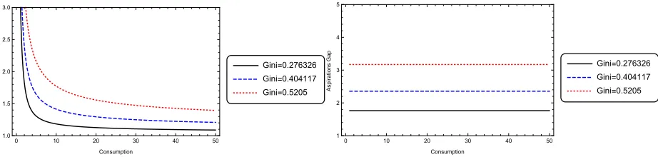
/∂ci but con-sider two examples commonly used in the inequality literature, Log Normal and Pareto. Figure

1 illustrates that ¯Ci/ci is monotonically decreasing in consumption level for Log Normal (left

panel). For Pareto (right panel), both rich and poor face the same aspirations gap. In both

cases, higher inequality implies a higher aspirations gap at all consumption levels. What is

dif-0 10 20 30 40 50

1.0 1.5 2.0 2.5 3.0

Consumption

A

spirat

ions

G

ap

Gini₌0.276326 Gini₌0.404117 Gini₌0.5205

0 10 20 30 40 50

1 2 3 4 5

Consumption

A

spirat

ions

G

ap

Gini₌0.276326 Gini₌0.404117 Gini₌0.5205

Figure 1: Consumption Deprivation for Log Normal (left) and Pareto (right)F_(c)

ferent in our model is that consumption inequality is the equilibrium outcome of an underlying

ability inequality. We show later that even for a Pareto distribution for ability, the equilibrium

consumption distribution behaves similar to the log Normal case. That is, the poor face a larger

margins from the static model in section 2.

Individuali’s preferences over consumption and leisure in periodtwhen he is alive are

ui t≡U(ci t, ¯Ci t,li t)=

c1_{i t}−σ

1−σC¯ ψσ i t +γ

(1−li t)1−σ

1−σ (11)

whereσ>0 and 0<ψ<1. This specification is similar to the macro KUWJ literature particularly

Gali (1994), though the consumption benchmark there is usually taken to be mean

consump-tion, same for all households. Forψ=(σ−1)/σwithσ>1, the first component of (11) becomes ¡

ci t/ ¯Ci t ¢1−σ

/(1−σ) similar to Abel (1990) where the aspirations level is mean consumption.

Alpizaret al.’s (2005) survey-experimental evidence shows that relative consumption of

non-positional goods matters as much as non-positional goods; no distinction is made here between

the two. We do allowψ6=(σ−1)/σwhich meansσ>1 is not necessary for an increase in ¯Ci t

to increase the marginal utility of consumption as long asψ>0. The quantitative results do,

however, use a value ofσabove unity to be consistent with the macro evidence.12

A final point about the utility function. Note that whenσ>1,ui t <0. To ensure that

util-ity from being alive always exceeds that from death, we normalize the latter to a large negative

number such thatU <inf©

U(ci t, ¯Ci t,li t) ª∞,N

t=0,i=1. A complete specification of individual

prefer-ences is then

U(ci t, ¯Ci t,li t)= 



 c1−σ

i t 1−σC¯

ψσ i t +γ

(1−li t)1−σ

1−σ , if agenti is alive

U, otherwise.

3.3 Decision Problem

Individuali’s labor productivityθi is time invariant, drawn at the beginning of his life from the

distributionΓ_{(θ) with finite support. We assume that the wage rate per efficiency unit of labor}

w is constant and exogenous. The return on investment ˜Ri t is individual-specific. Since

indi-viduals die over time, to ensure their assets are accounted for we assume a perfect annuities

market (Yaari, 1965). Under a perfectly competitive market, the zero profit condition implies

equilibrium annuitized investment return of ˜Ri t =R/φi t, R being the constant return on in-vestment. Implicitly this assumes access to an international capital market where the

borrow-ing and lendborrow-ing rates areR−1. This in turn implies a constant aggregate capital-labor ratio from

a CRS technology, and constant wage per efficiency unit of labor.

12_{Yet another alternative for socially-minded behavior is for agents to directly care about inequality measures}

Individuali’s periodtbudget constraint is

ci t+qi t+ai t+1=wθili t+R˜i tai t, (12)

whereadenotes his financial assets. He maximizes expected lifetime utility

E0

∞ X

t=0

βt "

Φ_{i t} (

c_{i t}1−σ

1−σC¯ ψσ i t +γ

(1−li t)1−σ 1−σ

)

+(1−Φ_{i t)U} #

, (13)

whereβ∈(0, 1) is the subjective discount rate, subject to the health transition equation (4),

health production function (5), survival function (7), budget constraint (12), and the usual

no-Ponzi game condition, given θi and initial conditions (ai0,Hi0). To conserve notation we do

not explicitly distinguish between calendar time and age of the individual even though not all

individuals will be alive every period. We are now in a position to note how the static model of

section 2 was a special case of this dynamic setup. It assumedψ=(σ−1)/σ,β=1,ξ=τ=ν=1,

ρ=1−α, δ=1 and exogenous ¯C. The health scale was redefined there to start at zero and

each household was initially endowed with (1−φ) ˜a/φassets to simplify the algebra, by ignoring the effect of health choice on the effective return on savings. Finally utility from death was

normalized to zero there which, for optimal decisions, is isomorphic to the assumptionv= −U.

Reformulate the decision problem above as a dynamic programming problem. Differently

from the Ramsey model with homogeneous KUWJ preferences, the entire consumption and

wealth distributions, not just their means, matter for households’ choices here. Since

individu-als face idiosyncratic productivity and aspirations levels, two simplifying assumptions are made

to reduce computational time and impose a recursive structure. First, we assume that the

in-dividual takes into account how his health choices affect the annuity return ˜Rthat he receives.

The rationale for this is that people often purchase insurance based on actuarial tables.13 Sec-ondly, we solve the household’s decision problem assuming the economy has reached the

sta-tionary distributions of health, wealth and consumption. Specifically we impose stationarity

of the consumption distribution, derive health and wealth dynamics consistent with that

as-sumption and then focus exclusively on the steady-state relationship between health, wealth

and aspirations.

Individuali faces four state variables (θi,ai t,Hi t, ¯Ci t) and three controls (ai t+1,li t,qi t) and

13_{It has the computational advantage of reducing the state space since the annuity return does not have to be}

his optimization decision is specified by the Bellman equation

V(θi t,ai t,Hi t, ¯Ci t)= max li t,ai t+1,qi t

©

u¡

ci t, ¯Ci t,li t ¢

+βφ(Hi t+1)V

¡

θi t+1,ai t+1,Hi t+1, ¯Ci t+1

¢

+β¡

1−φ(Hi t+1)

¢

Uª ,

(14)

V being the value of being alive, subject to

ai t+1=wtθi tli t+

R

φ(Hi t)

ai t−qi t−ci t,

Hi t+1=(1−δ)Hi t+Q(1−li t)αq_{i t}ρ,

¯

Ci t+1=C¯i t,

θi t+1=θi t=θi,

(15)

givenai0,Hi0andφi0=1. The third constraint says that the consumption distribution is

sta-tionary. It becomes relevant only when we turn to the quantitative results in section 4 below.

3.4 Optimal Behavior

Consider the optimal choices ofai t+1,li t, andqi t that follow from the decision problem (14).

First take the consumption Euler equation implied by the choice ofai t+1:

ci t+1 ci t

=¡βR¢1

σ

µ ¯

Ci t+1

¯

Ci t ¶ψ

. (16)

Since the interest rate is exogenous, to ensure a stable invariant distribution we impose the

restriction

βR=1 (A1)

under which the Euler equation simplifies to

ci t+1 ci t

=

µ ¯

Ci t+1

¯

Ci t ¶ψ

. (17)

This immediately implies that each individual’s consumption reaches steady state whenever

the aggregate consumption distribution is stationary as the individual’s relative position in the

consumption distribution remains unchanged over time. The perfect annuities market

Optimal choices for labor supply and health expenditure,li t andqi t, are

wθic−i tσC¯ ψσ

i t −γ(1−li t)

−σ_+β∂Hi t+1

∂li t £

φ′(Hi t+1){V(θi t+1,ai t+1,Hi t+1, ¯Ci t+1)−U}

+φ(Hi t+1)V3(θi t+1,ai t+1,Hi t+1, ¯Ci t+1)

¤

≤0,

(18)

and

−c_{i t}−σC¯_{i t}ψσ+β∂Hi t+1 ∂qi t

£

φ′(Hi t+1){V(θi t+1,ai t+1,Hi t+1, ¯Ci t+1)−U}

+φ(Hi t+1)V3(θi t+1,ai t+1,Hi t+1, ¯Ci t+1)

¤

≤0.

(19)

respectively. Define

Ω_{i t+1}≡φ′(Hi t+1)[V(θi t+1,ai t+1,Hi t+1, ¯Ci t+1)−U]+φ(Hi t+1)V3(θi t+1,ai t+1,Hi t+1, ¯Ci t+1),

the common term in equations (18) and (19), using which it follows from (19) that

Ω_{i t+1}= c

−σ i t C¯

ψσ i t β£∂Hi t+1/∂qi t

¤. (20)

Substituting (20) into (18) yields:

à _¯

C_{i t}ψ

ci t !σ

µ

wθi+ ∂Hi t+1/∂li t

∂Hi t+1/∂qi t ¶

=γ(1−li t)−σ. (21)

To make further progress, take the parametric example from (6) using which equation (21)

be-comes:

à _¯

C_{i t}ψ

ci t !σ

(1−li t)σ−1 µ

wθi(1−li t)− α ρqi t

¶

=γ. (22)

To understand how aspirations affect the individual’s health consider a simple comparative statics exercise. Suppose at the optimum governed by (22), individuali experiences an

exoge-nous increase in his aspiration level ¯Ci. How do health time investment and health expenditure

respond? Through the budget constraint, personal consumption is positively related to labor

supply, negatively to health expenditure. The remaining terms on the left-hand-side of (22), on

the other hand, depend negatively on labor supply and health expenditure. That is, the

left-hand-side of the equation is unambiguously decreasing in labor supply. When ¯Ci increases, an

increase in labor supply can restore equality to the first order condition. This means health time

The effect on health expenditure, on the other hand, is ambiguous. It could either rise or fall

depending on the strength of the response through consumption (denominator) versus returns to health expenditure (numerator). Recall, though, that health time and expenditures are

com-plementary inputs. Since health time investment falls unambiguously, there is another effect to

consider in the overall response to ¯Ci – returns to health expenditure fall. Indeed, for the special

case ofγ=0, equation (22) says that labor supply and health expenditure are inversely related

and the latter falls for sure. We conclude based on this, that a rise in aspirations lowers time

investment in health for sure and, possibly, health expenditures. Numerical simulations show

the latter is always true in the parameter space we consider. This is only a partial equilibrium

response since ¯Cidepends on the consumption distribution. It is important to understand how

the distribution responds in turn and affects equilibrium health and wealth outcomes. The definition below specifies this equilibrium which is then analyzed numerically in the following

section.

Definition 2. Thedynamic general equilibriumof this economy consists of a set of individuals

I_{t who are alive at t} =0, 1, . . . ,∞, a consumption distribution{Ci t}i∈I_t, controls{l_{i t},a_{i t+1},q_{i t}}

and state variables{θi,ai t,Hi t, ¯Ci t}for i∈It such that

(i) The controls{li t,ai t+1,qi t}represent the optimal solution to(14)subject to(15), given

{Hi t, ¯Ci t,ai t,θi},

(ii) The health stock evolves according to(6)for a given set of optimal controls{li t,ai t+1,qi t}

and Hi t, and

(iii) Aspirations are in equilibrium, that is, the distribution of aspirations{ ¯Ci t}taken as given

for the solution to(14)subject to(15)generates the distribution of optimal consumption

{Ci t}i∈I_t that is consistent with those aspirations according to(10),

given constant prices{w,R}and the initial distribution of{H0,a0}in the population.

The evolution ofI_{t follows the replacement assumption discussed in section 4.3. For now we}

note that a deceased individual is replaced by one with different labor productivity and initial

conditions.

4 Aspirations, Health and Inequality

To establish equilibrium relationships between aspirations and health behavior and between

inequality and aggregate health using quantitative methods, wherever possible parameter

4.1 Parameterization

Parameter values are reported in Table 2. Individuals are assumed to start their planning

hori-zon at age 20 which means all life expectancy numbers reported below are conditional on age

20. The length of a period is chosen to be a year, so the discount rate is set to 0.96, similar to

the business cycle literature. The implied return on saving is 4.17% consistent with long-run

US data. The weight on preference for leisure in the utility function,γ, is set to 0.5. The implied

average share of working hours is 0.35, close to the 0.36 implied by McGrattan and Rogerson’s

(2004, Table 1) estimate for 2000 assuming discretionary hours per day to be 16. We follow

Car-roll, Overland, and Weil (1997) in choosingσ=2. The aspirations parameterψis free and in

the baseline set to (σ−_1)/σ=_{0.5. This implies utility from consumption depends on the ratio} ci/ ¯Ci. Alternative values ofψare also considered. The depreciation rate of health capital is

taken to be 3% (Dalgaard and Strulik, 2014). Utility from death is normalized to−5000 so that

all households strictly prefer to be alive.14

Parameter Value Description Source

α 0.85 Leisure Parameter in Health Accu-mulation Equation

Match Life Expectancy Gap of 4.5 between top and bottom deciles

β 0.96 Discount Rate

σ 2 Elasticity of Substitution Carroll, Overland, Weil (1997)

Q 0.195 Health Investment Parameter Match Life Expectancy Gap of 4.5 between top and bottom deciles

τ 0.2 Shape Parameter for Probability of Survival

Match Life Expectancy Gap of 4.5 between top and bottom deciles

ξ 0.98625 Scalar Parameter for Probability of Survival

Match Life Expectancy Gap of 4.5 between top and bottom deciles

ν 0.1 Scalar Parameter for Probability of Survival

Match Life Expectancy Gap of 4.5 between top and bottom deciles

w 20 Wages Scale

Hi0 Varies Initial Stock of Health

ρ 0.15 Health good Parameter in Health Production

Match Life Expectancy Gap of 4.5 between top and bottom deciles

γ 0.5 Weight on Leisure Match average share of working hours

ψ 0.5 Strength of Reference Level of Consumption

Free

δ 0.03 Depreciation of Health Capital Dalgaard and Strulik (2014)

N 500 Size of the Population Scale

R 1/β Rate of Return on Savings

Table 2: Parameter Values

An individual enters periodt with an idiosyncratic labor productivityθ, financial assetsa,

14_{AsU becomes more negative, people acquire a greater distaste for death and invest more in health. The}

health capital H0, and an aspirations level ¯C that constitute the state-vector in his dynamic

programming problem (14). Since capital markets are perfect and complete and there are no non-convexities, long-run inequality in this economy depends on heterogeneous labor

produc-tivity alone that we refer to asfundamental inequality. The state spaceΘ_{for this productivity}

is discretized and agents are endowed with productivities ranging from 1 to 20 in increments of

κ=0.01. The probability/population weights corresponding to theθ’s are chosen from a Pareto

distribution. Since we are interested in tracing the effect of inequality on economic and health

outcomes, we use several combinations of the minimum and shift parameters of the Pareto

distribution.15

Since the initial population size and (exogenous) wage rate are scaling parameters, these

are set arbitrarily. To simulate each individual’s decision problem, he is endowed with an initial health close to his steady state and initial asset holding of zero. The former is arrived at by

solving the health transition equation (equation (4)) for a given set of policy rules. It ensures that

the simulations are local to the stationary distribution. In particular, since individuals die and

new individuals are introduced into the economy every period to replace them, it is possible

that a non-trivial measure of the agents never get close to their steady-state health and wealth

levels. Starting them at their steady-state health ensures faster convergence. The zero initial

assets assumption, on the other hand, is in keeping with a perfect annuities market where assets

of the deceased are seized by competitive risk-neutral firms.

To make plausible statements about the effect of aspirations on health behavior, we need to reasonably match life expectancy outcomes. Life expectancy gaps between the rich and the

poor differ substantially in the US and the gap has widened in recent decades (see for example,

Mearaet al., 2008 and Olshanksyet al., 2012). We follow Singh and Siahpush (2006) who

con-struct a relative deprivation index based on a number of indicators like education, occupation,

wealth and unemployment, a measure that is strongly correlated with relative income. They

re-port that the life expectancy at birth gap between the highest and lowest socio-economic status

increased from 2.8 years in 1980-82 to 4.5 years in 1998-2000 in the US. Since the simulations

are conducted in steady state, we target the latter number: values forα, ρ, Q, ν, ξ andτ are

picked in order that steady-state life expectancy gap between the top and bottom deciles is 4.5.

It is possible that several other combinations of these parameters also produce a similar life

15_{Most figures on aggregate inequality use the parameter combination {1.01, 1.01}. Since we truncate the upper}

tail of the Pareto distribution at 20, we redistribute the remaining weightω(forθ>20) over [1, 20]. Letxbe the rank ofθin the grid (Θ_{) over [1, 20]. Thenxgets assigned a new population weight ofG(x)}+ω.(x4/L), whereL=

P20/κ

1 x4is a normalizing constant,κis the step size of theΘgrid, andG(x) is the probability of drawing productivity

θ(x) from the untruncated Pareto distribution. The exponent on the re-weighting function and the mean ofΘ

are chosen to generate levels of inequality that are consistent with observed data. The resulting distribution still “looks” Pareto – for all of the distributions used in the simulations, the highest weight added to anyθ∈_{[1, 20] is}

expectancy gap. However, the computational demands of this problem are substantial. So we

fixedα,ρ, andQin order that health investment was large enough to keep the agent within the health state space, then variedν,ξ, andτuntil we achieved the desired gap. The shares of health

time and expenditures in health production,αandρ, are set at 0.85 and 0.15, respectively. We

have less guidance on these since estimates vary and have a large variance (e.g. Grossman,

1972b).

4.2 Baseline Results

Start with policy rules that map each household’s state vector (θi,ai,Hi, ¯Ci) into his choices

at a point in time. The existence of four state variables makes it difficult to present a policy

rule for all possible realizations.16 Since the objective is to uncover the effect of aspirations

operating through relative consumption, all decisions are plotted against the aspirations gap, ¯

Ci/ci. Each decision will be presented in three graphs corresponding to health stocks of 9, 10

and 11 units, to give an idea how they differ across health types. Unless otherwise noted, the

individual’s asset, one of the state variables, is set to zero. This does not qualitatively affect

the results presented below but cleanly isolates the role of labor productivity and exogenous

income differences.

Labor Supply and Health Production

Recall the analytical result from section 3 that agents with a larger aspirations gap, ¯Ci t/ci t, will

unambiguously supply more labor and most likely spend less on the health good. Confirming

that, Figure 2 shows that labor supply is increasing in the aspirations gap across health

lev-els17 andceteris paribusan increase in labor supply results in lower health. Could individuals

be substituting towards the health good as the aspirations gap rises? Not so: Figure 3 shows

that those with larger aspiration gaps also spend less on the health good. Doing so frees up

re-sources for personal consumption as these individuals attempt to close their aspirations gaps

while the discounted cost, in the form of worse survival, comes in the future. It is clear then from Figures 2 and 3 that an increase in the aspirations gap results in fewer inputs into health

production, worse health and higher mortality risk. While the existence of the gradient between

health inputs and the aspirations gap is independent of the individual’s health stock, the level

of investment is not. Both figures also show (note differing vertical scale) that, for a given

as-pirations gap, as the individual’s health stock deteriorates – for example if we move from panel

16_{The policy rules are plotted by calculating the aspirations gap, labor supply, health good, and savings for a}

given aspiration level, health stock, and assets.

17_{Some of the policy functions are not reported for the entire range of the aspirations gap because the gap does}

1.0 1.5 2.0 2.5 3.0 0.0 0.2 0.4 0.6 0.8 Aspirations Gap Labor S upply

(a) Health Stock: 9

1.0 1.5 2.0 2.5 3.0

0.0 0.2 0.4 0.6 0.8 Aspirations Gap Labor S upply

(b) Health Stock: 10

1.0 1.5 2.0 2.5 3.0

0.0 0.2 0.4 0.6 0.8 Aspirations Gap Labor S upply

(c) Health Stock: 11

Figure 2: Labor Choice vs Aspirations Gap

Solid:θ=1, Dashed:θ=5, Dotted:θ=15

(c) or (b) to (a) – he invests more in health production through lower labor supply and higher

expenditure on the health good.

1 2 3 4 5

0 5 10 15 20 25 30 35 Aspirations Gap Healt h G ood

(a) Health Stock: 9

1 2 3 4 5

0 5 10 15 20 25 30 35 Aspirations Gap Healt h G ood

(b) Health Stock: 10

1 2 3 4 5

0 5 10 15 20 25 30 Aspirations Gap Healt h G ood

(c) Health Stock: 11

Figure 3: Health Good vs Aspirations Gap by Health Stock

Solid:θ=1, Dashed:θ=5, Dotted:θ=15

Combining the implications of the previous two figures, Figure 4 shows that the individual’s

health stock worsens the larger is his aspirations gap and, controlling for the aspirations gap, he

invests more in health as his health stock falls.

To what extent are these effects due to the conventional effect of absolute income versus

socially-minded behavior? The best way to gauge that is to contrast two cases: the baseline

model (ψ=0.5) and a version without aspirations (ψ=0). Figure 5 presents labor supply and

health spending decisions as well as the implied changes in health stock as the aspirations gap widens. Labor supply, health expenditure and health outcomes strongly respond to relative

consumption when individuals care about their relative position. When they do not, relative

consumption has no health effect, only absolute income matters. The overall effect of

aspira-tions is thus to lower health production, an effect that worsens as one moves down the

con-sumption distribution, that is, for higher ¯Ci/ci.18

18_{The truncated Pareto distribution of productivity induces a consumption distribution for which ¯C}

1 2 3 4 5 -0.025 -0.020 -0.015 -0.010 -0.005 0.000 Aspirations Gap % Change in Hit

(a) Health Stock: 9

1 2 3 4 5

-0.025 -0.020 -0.015 -0.010 -0.005 0.000 Aspirations Gap % Change in Hit

(b) Health Stock: 10

1 2 3 4 5

-0.025 -0.020 -0.015 -0.010 -0.005 0.000 Aspirations Gap % Change in Hit

(c) Health Stock: 11

Figure 4: Percent Change in Health Stock

Solid:θ=1, Dashed:θ=5, Dotted:θ=15

1 2 3 4 5 6

0.0 0.2 0.4 0.6 0.8 1.0 Aspirations Gap Labor S upply

(a) Labor Supply

1 2 3 4 5 6

0 2 4 6 8 10 12 14 Aspirations Gap Healt h G ood

(b) Health Good

1 2 3 4 5

-0.025 -0.020 -0.015 -0.010 -0.005 0.000 Aspirations Gap % Change in Hit

(c) Percent Change in Health Stock

Figure 5: Aspirations and Health Production

Solid: Baseline, Dashed: No Aspirations

Savings Behavior

Return to the baseline model for the savings decision. Figure 6 shows that as the aspirations gap increases, the agent chooses to hold less assets. Beyond that, the savings decision exhibits

two interesting patterns. As the health stock declines, first, the gradient between the aspirations

gap and the level of savings gets flatter and second, the absolute amount of savings increases.

This is counter-intuitive since declining health should seemingly cause individuals to substitute

away from financial assets towards the health good and leisure. Assets, however, provide an

opportunity to improve health in the future. By saving, individuals can not only improve their

future health, they can afford higher consumption too. Both enable the individual to move

closer to his aspirations level in the future.19 This of course only highlights that financial saving

is not the sole way to provide for the future, health is an alternative.

Figure 7 plots the relationship between “full investment” and the aspirations gap. The

for-ci.

19_{The gradient between savings and aspiration gap is positive for the most productive individual in Fig 6(a). This}

1 2 3 4 5 6 0 2 4 6 8 10 Aspirations Gap S avings

(a) Health Stock: 9

1 2 3 4 5 6

0 2 4 6 8 10 Aspirations Gap S avings

(b) Health Stock: 10

1 2 3 4 5 6

0 2 4 6 8 10 Aspirations Gap S avings

(c) Health Stock: 11

Figure 6: Savings vs Aspirations Gap by Health Stock

Solid:θ=1, Dashed:θ=5, Dotted:θ=15

mer is calculated by adding the value of leisure time to health expenditure and financial assets,

that is, asRai/φi+wθ(1−li)+qi.20 Not surprisingly the relationship between this measure of

1 2 3 4 5 6

0 50 100 150 200 Aspirations Gap T ot al S avings

(a) Health Stock: 9

1 2 3 4 5 6

0 50 100 150 200 Aspirations Gap T ot al S avings

(b) Health Stock: 10

1 2 3 4 5 6

0 50 100 150 200 Aspirations Gap T ot al S avings

(c) Health Stock: 11

Figure 7: Total Savings vs Aspirations Gap by Health Stock

Solid:θ=1, Dashed:θ=5, Dotted:θ=15

overall investment and the aspirations gap is negative. Notably, comparing Figure 7 to Figure 6,

we see that a large proportion of full investment is allocated towards health; health is evidently

more valuable.

Life Expectancy

Next consider the effect that aspiration has on steady-state life expectancy for an individual.

Since those with the largest aspiration gap invest the least in health, we obviously expect them

to have lower life expectancy. Figure 8 looks at this by contrasting the baseline case of

aspi-rations (ψ=0.5) with one without (ψ=0) for the same productivity distribution. The level of

aggregate inequality as measured by the Gini coefficient is comparable in the aspirations and

no-aspirations scenarios, 0.45 and 0.43 respectively. Figure 8 shows that being aspirational has

20_{This is similar to Beckeret. al’s (2005) approach of valuing longevity gains to construct a measure of “full}

No Aspirations Aspirations

1.0 1.5 2.0 2.5 3.0

54 56 58 60 62

Aspirations Gap

Lif

e

E

xpect

ancy

Figure 8: Life Expectancy at Age 20 vs Aspirations Gap

a health cost. The highest ¯Ci/ci – the maximum aspirations gap in the figure – differs between

the aspirational and non-aspirational societies; the latter is smaller. In both scenarios, however,

this maximum corresponds to the same least productive individual since the distribution of

productivities is identical. Contrasting this individual’s life expectancy between the two

scenar-ios – a gap of about 3 years – clearly shows the adverse effect aspirations has on health. Another

way this is evident is in the population life expectancy gap. The gap between the lowest and highest deciles of the consumption ratio ¯Ci/ci (that is, between the most and least productive

individuals) is 6.87 with aspirations in Figure 8, significantly lower at 5.27 years without.

In summary, these results establish that relative position or consumption deprivation – as

measured by ¯Ci/ci– has a negative effect on an individual’s health because the greater marginal

valuation placed on personal consumption is met through less investment in health

produc-tion. That higher values of fundamental inequality imply greater aspirations gap in the

popu-lation means that higher inequality could lead to higher life expectancy gaps in the popupopu-lation

and, possibly, lower average life expectancy. A fuller appreciation of these results requires us to consider the general equilibrium implications.

4.3 Aggregate Implications

A positive measure of individuals die every period and are replaced by an equal number of new

agents each of whom draws his own productivity and starts with initial conditionsai0=0 and

Hi0= X(θi), where X is a function that produces the steady-state level of health for a given

of average consumption, labor, and the Gini coefficient. Typically these three variables reach

stationary values after 100 simulation periods. In what follows each of the simulations were run for 500 periods with a “burn-in” period of 500 which was dropped from the sample.

An important point to note before proceeding. In the closed-economy Ramsey model with

heterogeneous households, the steady-state wealth distribution requires a well-defined demand

for capital that is introduced through a diminishing returns production function (e.g.

García-Peñalosa and Turnovksy, 2014). Here, as in many open-economy models, the interest rate is

exogenous. To ensure a steady state, open economy models often assume an endogenous

dis-count rate, for exampleβas a function of consumption or income. In this model the effective

discount rate for any individuali, βΦ_{i, is endogenous. But the perfect annuities market}

as-sumption means expected return from saving and conas-sumption smoothing are independent ofΦ_{i. It is possible then fori to accumulate unlimited assets over time. Since the numerical}

solution method discretizes the state space for assets over a finite grid,i’s assets can converge

to the upper bound of that state space in finite time. Were that to happen, eventually the asset

distribution would become degenerate and all income heterogeneity would come from labor

income. In the simulations, however, only a tiny minority of high productivity individuals face

this issue. This is because mortality risk ensures that most individuals die well before reaching

the upper bound of the asset space. Moreover, when an individual dies, he is replaced by one

with no initial assets. Mortality and the replacement assumption together ensure that the vast

majority of agents are in the interior of the state space and the steady-state asset distribution is non-degenerate.

Is Inequality Motivating?

The first step in identifying the aggregate effect of aspirations is understanding their effect on

equilibrium income and consumption inequality. In other words, how does the consumption

and income inequality that result from aspirational behavior relate to fundamental inequality, inequality in endowed ability?

Milton Friedman posited inCapitalism and Freedom(1962) that inequality is desirable

be-cause, among other things, it motivates people to strive for something better. Presumably

do-ing so places them in a better position than otherwise. “Dodo-ing better”, in turn, can be taken to

mean better in terms of economic outcomes alone or overall welfare. Our model can be used

to test this claim since the aspirations gap – the gap between his personal consumption and

as-pirational consumption – motivates an individual to supply more labor and accumulate more

assets in order to increase income and consumption. Moreover, absent pecuniary externalities

We remove health from the model by settingτ=0 and first study how income for individuals

with differing productivities is altered by upward-looking aspirations. Evidently from Figure 9 (solid lines correspond to best non-linear fits), the drive to catch up motivates people to step up

their labor supply and realize higher steady-state income at all productivity levels.21But looking

closer, Figure 9 hints at a differential effect of aspirations across poorer and richer individuals –

the latter enjoy higher relative gains.

5 10 15 20

0 20 40 60 80 100 120 140

Income =

0

=0.5

Figure 9: Effect of Aspirations on Househo