Prediction of the Maximum Dislocation Density in Lath Martensitic Steel by Elasto Plastic Phase Field Method

Prediction of the Maximum Dislocation Density in Lath Martensitic Steel

by Elasto-Plastic Phase-Field Method

Zhenhua Cong

, Yoshinori Murata

, Yuhki Tsukada

and Toshiyuki Koyama

1_{Department of Materials, Physics and Energy Engineering, Graduate School of Engineering,}

Nagoya University, Nagoya 464-8603, Japan

2_{Department of Materials Science and Engineering, Graduate School of Engineering,}

Nagoya Institute of Technology, Nagoya 466-8555, Japan

On the basis of the two types of slip deformation (TTSD) model of lath martensite, the martensitic transformation was simulated in Fe­ 0.1 mass%C steel by an elasto-plastic phase-field method. The TTSD model allowed us to predict the total dislocations for the necessity of the formation of lath martensite, which is taken as the upper limit of dislocation density in lath martensite. The calculated dislocation density by the simulation was reasonable to be higher than the observed dislocations in value but to be the same in order. This consistence indicates that the calculation method based on the TTSD model is credible, together with the calculation of the habit plane predicted by the TTSD model. [doi:10.2320/matertrans.M2012067]

(Received February 20, 2012; Accepted June 25, 2012; Published August 8, 2012)

Keywords: dislocation density, slip deformation, phase-field method, lath martensite

1. Introduction

The martensite phase in steels exhibits several morphol-ogies such as lath, plate and butterfly, depending on the alloying elements.1,2) _{Among them, lath martensite exhibits}

high strength, wear resistance, and toughness.3­7) _The

martensitic microstructures must be characterized accurately in terms of orientation, morphology, transformation disloca-tion density, and retained austenite. In recent years, Morito

et al. observed the martensitic orientation and microstruc-tures by means of TEM, SEM and EBSD.8­11)_{Spanoset al.}

adopted EBSD and serial sectioning to establish 3-D mor-phology of martensite lath,7)which provided further detailed insights into lath orientation, distributions and shapes.

High dislocation density is inevitable in lath martensite, which accommodates the large strain induced by martensitic transformation and subsequent interface gliding. Wayman classified the dislocations in the martensite phase into two types: transformation dislocations and interface disloca-tions.5) _{Morito et al. used a TEM method to measure the}

dislocation densities in nickel steels and carbon steels, and they reported that the dislocation density for lath martensite is approximately 1.11©1015_m¹2 _{in a Fe­0.18C steel and}

3.8©1014_m¹2_{in a Fe­11Ni steel.}12)_{In addition, Conget al.}

used the X-ray diffraction (XRD) method to detect the dislocation density of lath martensite in low carbon steels (0.02­0.09 mass%C) and the dislocation density is 4.87© 1014m¹2 in a Fe­10Cr­5W­0.02C steel.13) However, all these studies focus purely on experimental results, which cannot relate the dislocation with the formation mechanism of lath martensite.

Recently, Iwashita et al. developed a two types of slip deformation (TTSD) model to explain the formation mechanism of lath martensite.14) _{In this model, high}

dislocation density introduced by martensitic transformation is realized by two inevitable independent slip systems. In this

study, the total dislocations for the necessity of the formation of lath martensite steel is counted by simulation using an elasto-plastic phase-field model based on the TTSD model, and the result is compared with the experimental results reported until date.

2. Evaluation of the Maximum Dislocation Density Based on the TTSD Model

According to Iwashitaet al., the martensitic transformation is accomplished by coupling lattice deformation and plastic deformation.14) _{The lattice deformation (Bain deformation)}

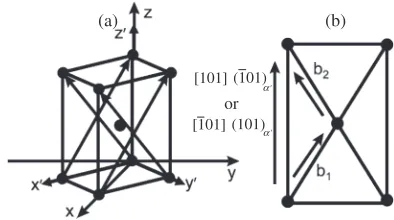
realizes the transformation from the austenite phase with a face-centered cubic (fcc) lattice to a body-centered tetragonal (bct) lattice. After that, the length of thec-axis is adjusted to accommodated the strain induced by Bain deformation. Due to the strain induced by Bain deformation is so large that plastic deformation is inevitable. In the present study, the plastic deformation is realized by dislocation slip along two independent slip systems as shown in Fig. 1, which is called as the TTSD model. The crossed planes shown in Fig. 1(a) are the two types of slip systems, ½101ð101Þ_¡0 and

½101ð101Þ_¡0.14) Through TTSD model, the habit plane

{557}_£ and lattice correspondence between the martensite

or '

'

(a) (b)

[101] (101)

α

[101] (101)_α

Fig. 1 Skeleton of plastic deformations along two slip systems, i.e.,

½101ð101Þ_¡0 and½101ð101Þ_¡0.b₁andb₂are the Burgers vector for the

two slip systems.

phase and the austenite phase are successfully explained without any rotation matrix. Figure 1(b) shows that each slip system can be taken as a combination of two a=2h111i_¡0

dislocation slips with the Burgers vectors ofb1andb2, which

can usually be observed in practical steels. Compared to directly performing the slip deformation along h111i slip system, the TTSD model can represent the plastic deforma-tion simply. Moreover, the TTSD model can well explain the {557}£ habit plane in the formation process of lath martensite.

Assuming that the plastic deformation is accommodated throughoutly by these dislocation slips, the total dislocations for the necessity of the formation of the lath martensite can be evaluated. The idea for using the phase-field method to model a dislocation is establishes by Nabarro15) _that

dislocations can be taken as a set of coherent misfitting platelet inclusions. For simplisity, a dislocation loop is described as a sheared pletelet with thickness and the region inside the platelet is sheared by a Burgers vector b.16) _By

extending this discription to a spatial region with a population of dislocations, the average plastic strain pave, caused by dislocation slip is given by

pave¼

jbj

D ; ð1Þ

where «b« is the magnitude of the Burgers vector andD is the average distance between the neighboring slip planes, that is, dislocation planes. In the formation process of lath martensite, a lot of dislocations are necessary for the plastic accommodation. After the martensitic transformation, some dislocations are resided in the martensite crystal, which can be observed by experiments, whereas some dislocations pass through out of the martensite crystal using for the formation of lath boundaries, which cannot be observed directly by experiments. In the present study, we focuses on the total dislocations contributing on the formation of lath martensite, which is taken as the upper limit of dislocation density of lath martensite, μlim. In the martensitic transformation, μlim should contribute to the plastic deformation for moderating the strain by Bain lattice deformation. Here, we give the distance between neighboring dislocations by a rough estimation as

D1= ffiffiffiffiffiffiffiffiμlim

p

: ð2Þ

Assuming that all of the dislocations contriute to the plastic deformation, the value of D can be estimated from the average plastic strain pave, which is available from the

simulation results by using phase-field model. As mentioned above, TTSD model is based on ½101ð101Þ_¡0 and

½101ð101Þ_¡0 slip systems in bct crystals as shown in

Fig. 1(a). Therefore, the value of D evaluated from eq. (1) is the distance between the neighboring slip planes along ½101ð101Þ_¡0 or ½101ð101Þ_¡0. To obtain the total dislocations

for the necessity of the formation of martensite phase in a real case, the value ofDalongh101i_¡0 should be transformed to

the value alongh111i_¡0, as shown in Fig. 1(b).

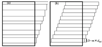
For a real case, the slip planes should arrange randomly as shown in Fig. 2(a). For simplicity, it is assumed that the intervals between neighboring slip planes are the same, as shown in Fig. 2(b). If the number of lattice planes between

two adjacent slip planes for each slip system is m, then the value of Dcan be given by eq. (3):

D¼mdhkl: ð3Þ

The distance between the (hkl)_¡Aplanes can be obtained from eq. (4).

dhkl¼

1 ffiffiffiffiffiffiffiffiffiffiffiffiffiffiffiffiffiffiffiffiffiffiffiffiffiffiffiffiffiffi

h2 a2 ¡0

þk2 a2 ¡0

þ l2 c2 ¡0

s ; ð4Þ

whereh,kandlare the Miller indices of the slip planes, and

a¡Aand c¡Aare the lattice parameters of the martensite phase. By inserting the values ofD(101) estimated from eq. (1) and

d(101)in eq. (3), we can evaluate the number of lattice planes

slipping along the h101i_¡0 system, m₍₁₀₁₎. As a result, the

number of lattice planes slipping actually along the h111i_¡0

directionm(111)should be twice that ofm(101). By substituting

the values ofm(111) and d(111) into eq. (3), we obtain D(111).

Now with the help of D(111) and eq. (2), the total amount

of dislocations for the necessity of the formation of lath martensite in practical steels can be evaluated.

3. Elasto-Plastic Phase-Field Method

For the martensitic transformation, thefield variable º_iðrÞ (i=1, 2, 3) is introduced to describe the Bain deformation and i=1, 2, 3 is used to distinguish the three coordinate coincidences; that is, thec-axis of the bct phase is along the three equivalenth100idirections in the austenite matrix. Here

ris the positional vector.º_iðrÞ(i=1, 2, 3) ranges from 0 to 1 and 0 represents austenite phase, where 1 represents the full martensite phase at a certain i. In the present simulation, the lath martensite phase is formed only when º_iðrÞ²0.7. Another field variable p¡_iðrÞ (i=1, 2, 3) is considered to describe the plastic deformation and the value of p¡_iðrÞ represents the local plastic strain produced by dislocations.

¡represents the number of slip systems, i.e.,½101ð101Þ_¡0 or

½101ð101Þ_¡0. In our simulation, the value of p¡

iðrÞ ranges from 0, which means no plastic deformation, to 1.21, which is the maximum of plastic strain determined by eqs. (1) and (3). The plastic deformation will choose the slip system, which has the bigger value of p¡_iðrÞ, to accommodate the strain caused by Bain deformation.

The martensitic transformation is a minimization process of the total free energy for the phase-field simulation. Here the total free energy is defined by the Ginzburg­Landau-type Gibbs free energy functional, which is a sum of chemical free

energyEchem, gradient energyEgrad, and elastic strain energy Eel:17)

Etotal¼EchemðfºiðrÞgÞ þEgradðfp¡gÞ þEelðfºiðrÞg;fp¡gÞ: ð5Þ

The chemical term is taken as the driving force for martensitic transformation, which can be approximated by the conventional Ginzburg­Landau phenomenological coarse-grained functional of field variables. It contains the local specific free energy and non-local gradient terms, i.e.:18)

Echem¼

Z

r

f0ðfºiðrÞgÞ þ

¼

2 X3

i¼1

ðrºiðrÞÞ2

" #

dr; ð6Þ

wheref0 is the specific free energy and is defined as

f0¼f

a 2

X3

i¼1

º2

i b 3

X3

i¼1

º3

i þ c 4

X3

i¼1

º2 i !2 8 < : 9 = ;: ð7Þ

Here,a,bandcare the coefficients of the Landau polynomial

expansion. In this study, they are chosen as a=0.1,

b=3a+12 and c=2a+12.17) ¦f is the driving force for the martensitic transformation, which is calculated by Thermo-Calc with CALPHAD method. The second term in eq. (6) is the gradient part due to the inhomogeneity of the

field variable ºiðrÞ. ¬º is a coefficient positively defined

second-rank tecsor andr @=@ri is a differential operator. The gradient energyEgraddescribes the contribution of the

core energy of the dislocations to plastic accommodation an it is represented by the following equation:16)

Egrad¼¬p

2 Z

r

X3

i¼1

X

¡ ½n¡

ðiÞ rp¡ðiÞ ½n¡ðiÞ rp¡ðiÞdr; ð8Þ

where ¬p is the gradient energy coefficient to guarantee a smooth transition of the deformation strainfield profile on the austenite/martensite interface andniis the unit vector of the slip plane normal.

According to Khachaturyan,19)the elastic strain energy is given by

Eel¼

1 2 Z

r

Cklmnf¾klðrÞ ¾0klðrÞgf¾mnðrÞ ¾0mnðrÞgdr; ð9Þ

where Cklmn is the elastic coefficient matrix. For simplisity,

the material is assumed to be isotropic due to that the elastic constants of lath martensite are not available up to date. Therefore, the tensor Cklmn can be expressed as Cklmn¼

­¤kl¤mnþ®ð¤km¤lnþ¤kn¤lmÞin terms of the Lamé constants

­and®, which are estimated from Young’s modulus and the Bulk modulus for an isotropic cubic crystal.20)_{Here, ¤(x) is}

the Dirac delta function. ¾klðrÞ is the total strain, which is defined as the sum of the homogeneous strain ¾kl and the heterogeneous strain¤¾kl:

¾klðrÞ ¼¾klþ¤¾klðrÞ: ð10Þ

¾kl describes the macroscopic shape deformation of the system. When the macroscopic shape of the system isfixed during the transformation, the homogeneous strain is zero.16)

The heterogeneous strain ¤¾kl, is defined to satisfy

R

V¤¾kl¼0. According to the theory of elasticity,

19) _{¤¾kl is}

given as

¤¾klðrÞ ¼

1

2fmkðrÞnlþmlnkðrÞg·

0

mnðrÞnn; ð11Þ

where ·0

mn Cklmn¾0kl. ³km(r) is the Green function tensor

and is defined as below21)

mkðrÞ ¼¤_®mk_2®n_ðmnk

1¯Þ: ð12Þ

¾0

klðrÞis the total eigen strain and is given by

¾0 kl ¼

X3

i¼1

ð¾B

klðiÞ ºiðrÞÞ

þX

¡

b¡

i n¡i þn¡i b¡i

2jb¡_ij p

¡ iðrÞ

; ð13Þ

where thefirst term describes the eigen strain caused by the Bain deformation and the second term is the eigen strain attributed to the plastic deformation. By inserting all the terms to eq. (9), the elastic strain energy can be evaluated. As a result, the total free energy Estr, for the martensitic transformation is determined.

The dynamics of martensitic transformation is controlled by the Allen­Cahn equation:22)

@Mðr; tÞ

@t ¼ LM

¤Etotal

¤Mðr; tÞ; ð14Þ where M(r, t) ðM¼ºi; p¡iÞ are the field variables of the coordinate vectorrand evolution timet, andLMis the kinetic parameter of each field variable.

4. Numerical Simulation

The evolution of lath martensite in Fe­0.1 mass% C steel was simulated at 300 K by the elasto-plastic phase-field model in 3-D space. The simulation was performed in a cubic with N3 (N=64) meshes and the mesh size is 4 nm. Therefore, the computational domain is 256©256© 256 nm. For the initial state, a dislocation loop with a radius of 12 nm is set in the center of the austenite cubic and the growth of lath martensite with time evolution is simulated around the dislocation loop. The shape of the martensite lath is taken as a thin plate with thickness. The time step ¦t*is set to be 0.001 and the symbol of asterisk represents a dimensionless simulation time. The lattice parameters both of the austenite phase and martensite phase are estimated to be a_£=3.599©10¹10_{m, a}

¡A=2.867© 10¹10_{m and c}

¡A=2.880©10¹10m, respectively, in Fe­ 0.1 mass%C steel. Assuming the calculation system is isotropic, the Lamé constants ­ and ® are estimated to be 123 and 72 GPa from both the Young’s modulus and the Bulk modulus of pure iron.23) The driving force for the martensitic transformation,¦fis calculated to be 5085 J/mol in a Fe­0.1 mass%C steel at 300 K based on Thermo-Calc data base. The gradient coefficients with respect to the

field variables ºiðrÞ and p¡iðrÞ are fitted to be 1.6©

10¹14_J·m2_{/mol and 30©10}¹14_J·m2_{/mol, respectively. The}

5. Results and Discussion

Figure 3 shows the time evolution of the average value of plastic strainpave. It considers all the local values of plastic

strain in lath martensite along the two slip systems, ½101ð101Þ_¡0 and ½101ð101Þ_¡0. The figure reveals that the

average plastic strain increases with the progression of martensitic transformation and saturated in 30 time steps at a value of 0.036. This means that the martensitic trans-formation is accomplished att*=30. Therefore, we use the saturated value of pave to estimate the maximum dislocation density in a full lath martensite. By inserting the values of

pave and «b(101)«=4.06©10¹10m in pure iron into eq. (1),

we calculate the distance between neighboring slip planes

D(101) to be 1.13©10¹8m. Substituting the values of D(101)

anddð101Þ_¡0 =2.03©10¹10m into eq. (3), the value ofm(101)

is estimated to be 56, and thus m(111)should be 112 for the

actual slip systems in the martensite phase. By substituting the values ofm(111)anddð111Þ_¡0 =1.66©10¹10m into eq. (3)

again, we calculated D(111) to be 1.86©10¹8m. Once the value of D(111) is known, the maximum dislocation density in a practical steel is evaluated to be 2.89©1015m¹2 from eq. (2). The simulation result is almost twice that of the experimental result in a Fe­0.1 mass%C steel (1.55© 1015_m¹2_{) measured by Kehoeet al.using a TEM method.}24)

The simulation result is definitely higher than the exper-imental result with respect to the value, but the orders of the dislocation density are the same. As mentioned in Section 2, the maximum dislocation density μlim considers the total dislocations for the necessity of the formation of lath martensite. In this sense, the calculation result is natural and right higher than the observed dislocation density.

In our calculation, only the dislocations in the martensite phase are considered. In fact, the surrounding austenite phase should also contain some dislocations because of the strain originating from the martensite phase and they may be inherited into the lath martensite phase during martensitic transformation.5)However, it is argued that if the surrounding austenite phase is deformed during martensitic transforma-tion, it will help to accommodate part of the strain in the martensite phase, thus resulting in the loss of dislocation density in the martensite phase itself. This loss and the

Fig. 3 The average value of the plastic strain pave along the two slip systems.

A

dislocations stored in the surrounding austenite phase cancel each other out. Therefore, the maximum dislocation density in a full martensite should be almost equal to our result. In other words, during martensitic transformation, the total strain containing the surrounding austenite phase is consid-ered to be represented by the dislocations in this study, although the quantitative evaluation should be done in the future.

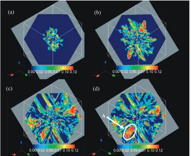
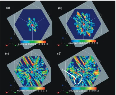
Figures 4 and 5 show the time evolution of the local plastic strain p¡_iðrÞ (i=1, 2, 3) along the½101ð101Þ_¡0 slip system

and the ½101ð101Þ_¡0 slip system on the {111} plane by

phase-field simulation, respectively. In Figs. 4 and 5, the deep blue areas indicate that there are no slip deformation, while the red areas represent the most dramatic slip deformation. For a specific value shown in Figs. 4 and 5, it may come from an arbitrary lattice corresponding in Bain deformation, where the value of ican be equal to 1, 2 or 3. But all the values distributed in a packet contain the local plastic strain for all the three cases of lattice corresponding, i.e.,i=1, 2 and 3. Because of a dislocation loop set in the center of the austenite phase as the initial state, the slip deformation also originated from the center of the austenite phase and the range of the slip deformation extends with the evolution of the martensitic transformation. It is to be noted that the plastic strain of area“A”marked in Fig. 4(d) is very large, while in the same area “B”marked in Fig. 5(d), there is almostly no plastic strain along the other slip system. This result can be observed at all times and places by comparing Figs. 4 and 5. So it is concluded that the slip

deformation along the two slip systems are complementary and they cooperated with each other to assist the plastic accommodation.

6. Conclusions

The maximum dislocation density of lath martensite in a Fe­0.1 mass%C steel was evaluated on the basis of a TTSD model. By employing an elasto-plastic phase-field method based on the TTSD model, the average value of plastic strain was evaluated to be approximately 0.036 for 30 time steps. The evaluated maximum dislocation density was 2.89© 1015_m¹2_{. This result was reasonable to be higher than the}

observed dislocation density in value but to be the same in order.

REFERENCES

1) G. Olson and W. Owen: Martensite, (ASM International, Materials Park, Ohio, 1992).

2) K. Otsuka and C. M. Wayman:Shape Memory Materials, (Cambridge University Press, Cambridge, 1999).

3) K. Wakasa and C. M. Wayman:Acta Metall.29(1981) 973­990. 4) K. Wakasa and C. M. Wayman:Metallography14(1981) 49­60. 5) B. P. J. Sandvik and C. M. Wayman:Metall. Trans. A14(1983) 809­

822.

6) P. M. Kelly: Mater. Trans., JIM33(1992) 235­242.

7) D. J. Rowenhorst, A. Gupta, C. R. Feng and G. Spanos:Scr. Mater.55 (2006) 11­16.

8) S. Morito, X. Huang, T. Furuhara, T. Maki and N. Hansen:Acta Mater. 54(2006) 5323­5331.

B

9) S. Morito, H. Tanaka, R. Konishi, T. Furuhara and T. Maki:Acta Mater. 51(2003) 1789­1799.

10) S. Morito, I. Kishida and T. Maki:J. Phys. IV France112(2003) 453­ 456.

11) S. Morito, H. Saito, T. Ogawa, T. Furuhara and T. Maki:ISIJ Int.45 (2005) 91­94.

12) S. Morito, J. Nishikawa and T. Maki:ISIJ Int.43(2003) 1475­1477. 13) Z. Cong and Y. Murata:Mater. Trans.52(2011) 2151­2154. 14) K. Iwashita, Y. Murata, Y. Tsukada and T. Koyama:Phil. Mag. 91

(2011) 4495­4513.

15) F. R. N. Nabarro: Phil. Mag.42(1951) 1224­1231.

16) N. Zhou, C. Shen, M. Mills and Y. Wang:Phil. Mag.90(2010) 405­ 436.

17) A. Yamanaka, T. Takaki and Y. Tomita:Mater. Sci. Eng. A491(2008)

378­384.

18) Y. Wang and A. G. Khachaturyan:Acta Mater.45(1997) 759­773. 19) A. G. Khachaturyan:Theory of Structural Transformations in Solids,

(John Wiley and Sons Inc., New York, 1983).

20) W. Zhang, Y. M. Jin and A. G. Khachaturyan:Acta Mater.55(2007) 565­574.

21) Y. M. Jin, A. Artemev and A. G. Khachaturyan:Acta Mater.49(2001) 2309­2320.

22) J. Kundin, H. Emmerich and J. Zimmer:Phil. Mag.90(2010) 1495­ 1510.

23) Japan Institute of Metals: Metals data book, third ed., (Maruzen, Tokyo, Japan, 1993).