Improving the Planning of Train
Infrastructure Maintenance
[1]
[2]
Improving the Planning of Train Infrastructure Maintenance
CREATING INSIGHT IN THE EXPERIENCED NUISANCE AND FINANCIAL IMPACT OF TRACK POSSESSIONS BY OPTIMIZING THE MAINTENANCE PLANNINGVersion: Version 8,2
Author: Laurent Knook | 06-55544768 | [email protected] University: University of Twente
Study: Master Industrial Engineering & Management Track: Production & Logistics Management
Faculty: Behavioural Management and Social Sciences
Graduation committee:
University of Twente: Dr. M.C. van der Heijden
Faculty of Behavioural Management and Social Sciences Dep. Industrial Engineering and Business Information Systems
Dr. E. Topan
Faculty of Behavioural Management and Social Sciences Dep. Industrial Engineering and Business Information Systems
ProRail: H.C. Zandman Manager BTD
Operatie, Assetmanagement, Infrabeschikbaarheid
[3]
Management Summary
The motivation for our work is the challenge ProRail is having with their maintenance planning process. The main problem is that standard practice at Prorail is to not plan more than 4 years ahead. This leads to a lack of overview for tactical decisions and unused opportunities to reduce nuisance. Nuisance will be based on the expected number of passengers during track work multiplied by the amount of experienced nuisance. The experienced nuisance is based on the expected extra time people travel by bus or train, when there is track work. When track work is done, a part of rail infrastructure is reserved for that purpose. This is called a possession.Possessions signify which tracks are out of service, at what date and for what duration.By moving possessions from various years to the same year possessions could be clustered together, and as such reduce the amount of nuisance. Moving possessions will induce some cost, for example for extra maintenance or the early write-off of assets. We use a fictive cost model, to proof the benefits of our
planning process. Our main goal is to create a method which determines which possessions, from a period of five years, should be performed together. This method should be able to optimize the balance between induced experienced nuisance for passengers and financial impact (and steer tactical decision making on track work planning). The possessions that are considered are those longer than four hours and which can be planned two years ahead. Furthermore, we will look at combining possessions that are on unique parts of tracks that can be completely replaced by busses or a detour. For our approach we created an integer linear model, which is solved using CPLEX and a compound heuristic. The compound
heuristic consists of a greedy construction heuristic and two local search steps: Steepest Hill Climbing and Simulated Annealing. Our findings are that CPLEX could be used in the
[4]
Content
Chapter 1: Introduction1.1 ProRail ... 6
1.2 Problem definition ...12
1.3 Research Questions ...16
1.4 Overview of the thesis ...17
Chapter 2: Literature review 2.1 Review ...18
2.2 Conclusion ...22
Chapter 3: Problem modelling 3.1 Model description ...23
3.2 Example of the model ...26
3.3 Mathematical Formulation ...30
3.4 Conclusion ...32
Chapter 4: The solution method 4.1 Constructive heuristic ...33
4.2 Improvement heuristic ...35
4.3 Conclusion ...39
Chapter 5: Computational study 5.1 Experimental design ...41
5.2 Performance of the construction heuristic ...44
5.3 Performance of the two local search heuristics ...47
5.4 Case: Den Haag HS – Rotterdam Central (2013-2017) ...49
5.5 Conclusion ...54
Chapter 6: Conclusion & Recommendation 6.1 Conclusion ...55
[5]
Glossary
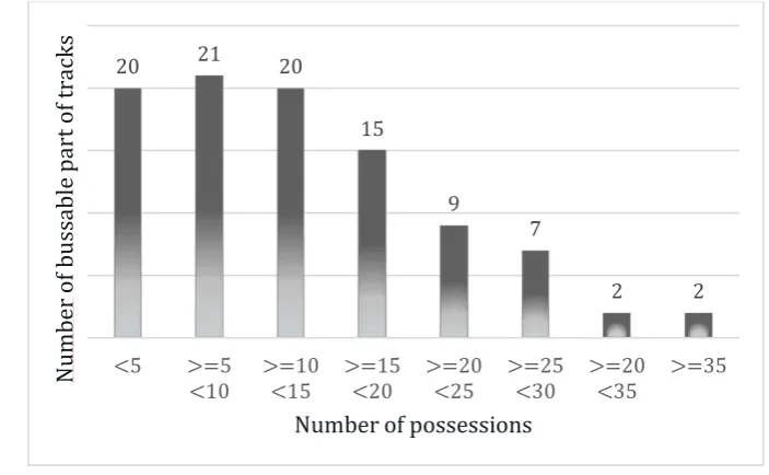
Bussable part of track A bussable part of track is the combined amount of track that can stillbe replaced by busses or a detour, as defined by NS. The Netherlands is divided into 96 unique bussable part of tracks, without any overlap. Each bussable part of track consist of multiple uninterrupted track segments. All the bussable part of tracks can be found in Appendix Bussable part of tracks F.
Clustering By clustering two or more possessions, we assume that they will be performed at the same time. Multiple possessions in one cluster on the same bussable part of track lead to a reduction in nuisance.
Combining See clustering.
ETM Measurement for experienced amount of extra travel time for a train passenger due to a possession at ProRail “Dutch: Ervaren reizigers minuten”.
Nuisance The amount of experienced nuisance a possession gives on a bussable part of track. In our research nuisance will be measured using ETM multiplied with the expected number of passengers during a possession on that bussable part of track.
Pm The measurement for nuisance is in pm (passenger * minutes). Which tells how many passengers, experience how many minutes of
nuisance.
Possession Moments that are used for track works are called possessions. A possession could contain various type of track works at the same time. One or more track segments could be occupied during a possession. Track segment A track segment is used to refer to all parts of the rail infrastructure
[6]
1.
Introduction
In this thesis we will suggest a method for improving the train maintenance planning process at ProRail. We will first introduce ProRail and explain the current maintenance planning. This will lead to the formulation of our research questions. Finally, we will give an overview of the structure of the rest of the thesis.
1.1
ProRail
1.1.1 Description of ProRail
The mission of ProRail is to enable pleasant travel and sustainable transport, and to connect people, cities and companies, now and in the future. ProRail is responsible for the Dutch rail infrastructure: construction, maintenance, management and safety. They control all train traffic and build and manage all stations and tracks. To give an impression of the complexity of this objective, the Dutch rail infrastructure contains 7.219 km of track, 404 stations, 56 bridges, 15 tunnels, 12.092 signals, 7006 switches and 2368 railroad crossings. On average, there are 1,1 million passengers per day and 3,3 million freight transport trains per year (ProRail, 2016).
ProRail has the following functions:
a) Deliver train paths (construction and maintenance) b) Capacity management (management)
c) Controlling of rail traffic (safety)
a) To deliver train paths, the required infrastructure to go from A to B, ProRail is responsible for the construction and maintenance of the infrastructure. The clients of ProRail are the railway undertakings: passenger transporters, freight transporters and maintenance control companies. To deliver these train path, the infrastructure is maintained, renewed and
modified. All the work on the infrastructure is outsourced by so-called “performance
[7]
Figure 1 flow diagram of products, client and supplier. (Jonge, 2018)
b) Capacity management is the task of determining when, what infrastructure is used for which function. The function could for example be: transporting passengers or maintaining the infrastructure. This is difficult, because there is a constant conflict between improving the infrastructure and using the infrastructure.
c) Controlling of rail traffic, ProRail is controlling all passenger and freight trains. There are thirteen traffic control centres throughout the Netherlands. They make sure that all trains leave and arrive on time. Furthermore, they are the centre of management during calamities and try to reduce the amount of conflicts that arise.
The goal of this thesis is to improve the availability of train paths. The department Possessions (In Dutch: Buitendienststellingen) is the client of this research. How this
[8]
[9]
1.1.2 Current planning process at ProRail
The planning of possessions involves various departments of ProRail, both regional and national. The process involves more than 200 people, and many decisions. Among others: “what assets need maintenance?”, “what type of renewal should ProRail do?”,“when do they need maintenance?”, “can we cluster them with other possessions?” and“is there enough work capacity on the market to do all the possessions?”. All these different aspects make the planning of work on the infrastructure a very complex process. We will first explain the various type of work on the infrastructure, following on this we will explain how the various type of work are planned, and which departments are involved.
Work on the infrastructure, track works, can be categorized into two major classes: (i) maintenance and (ii) renewal. Within maintenance the two categories are: preventive and corrective maintenance. An overview of all the type of track works can be seen in Figure 3.
Figure 3: Possession requirement for maintenance and renewal of railway infrastructure adapted from (Paragreen, 2010) taken from (Famurewa, 2015)
a) Maintenance
Preventive maintenance itself can be categorized into two classes: Predetermined maintenance and Condition-Based Maintenance (CBM). CBM is being performed given a certain input reaching a threshold. The type of input could be sensor data or any other direct monitoring method. Given a certain condition, the maintainer will plan a maintenance possession. At ProRail for example, monitoring could be: measuring the thickness of the overhead line. The corresponding condition is then: if the line is thinner than
one-centimetre, initiate action. The corresponding action is: replace the overhead line. We will also include age-based maintenance. At ProRail, if an asset is a certain number of years away from the theoretical replacement age, the asset will be inspected. If the condition of the asset is not up to standards it needs to be replaced, otherwise a new age will be determined. A classical assumption in CBM modelling is that the system failure can be explained by a deterioration process (Ahmad & Kamaruddin, 2012; Deloux, Castanier, & Bérenguer, 2009). Predetermined maintenance is also known as systematic preventive/time-based
[10]
of system failure. TBM policies are developed based on historical failure data (Alaswad & Xiang, 2017)
Corrective maintenance, is a reactive approach to maintenance because the action is triggered by an unscheduled event. This type of maintenance has a high priority because failure is most common cause for those maintenances. Therefore, this maintenance must be done urgently, therefore the scheduling and planning of this type of maintenance is difficult to do in advance.
b) Renewal
At ProRail, renewal is divided in change of function and local projects. Change of function includes possessions that involve a change in the current rail infrastructure network. For example, if the railway undertakers (passenger transporters, freight transporters) would like to drive more trains on a route, this could imply an extra railroad switch should be placed. Placing this switch is a change of function. Local projects are infrastructure projects initiated in the Netherlands by local governments who would like to alter the surroundings of the rail. For example: removing a crossing, placing a tunnel or placing a sound wall. Each possession result in delay experienced by travellers. Nuisance is the amount of
deviation in travel time compared to the normal train service times the number of expected passengers. At ProRail, the amount of deviation in travel time is measured in extra amount of experienced travel time (ETM). ProRail, Locov1 and NS together created estimations for
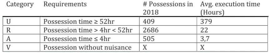
[image:11.595.81.512.522.608.2]extra travel time for each part of track in the Netherlands if it would be out of service. ETM is based on how many minutes of extra travel time a passenger experiences whether he/she needs to take busses or a detour. Furthermore, within ProRail there are different categories for the duration of a possession. An overview of the different categories can be seen in Table 1. The separation at 52 hours comes from the amount of work that can be performed in a weekend as defined by ProRail. It starts on Saturday at 1:00 and ends on Monday at 5:00.
Table 1 Nuisance categories from ProRail
Category Requirements # Possessions in
2018 Avg. execution time (Hours)
U Possession time ≥ 52hr 409 379
R Possession time > 4hr < 52hr 2686 22
A Possession time ≤ 4hr 505 3,7
V Possession without nuisance X X
1 Locov is a collaboration of consumer organizations where they represent the interests of the train
[11]
1.1.3 Planning of various type of maintenance
The track works planning process for rail infrastructure can be described in eight steps: 1) Budget determination, 2) Long-term quality prediction, 3) Project identification and
definition, 4) Project prioritization and selection, 5) Possession allocation and timetabling of track possession, 6) Project combination, 7) Short-term maintenance and project
scheduling, 8) Work evaluation and feedback loop (Budai-Balke, 2009). In this thesis the focus will be on step 3 up to step 6, these steps are structured at ProRail as show in Figure 4
Figure 4: Three steps to describe the current track planning process at ProRail. With the steps above associated with the steps identified, for describing the planning process, by (Budai-Balke, 2009)
At ProRail, possessions smaller than 4 hours are planned in a different way compared to the category type R and U possessions. There is a separate schedule in which type A possessions are planned. This type of possessions are mainly below four hours. There are fixed routine nights in which these possessions can be performed, as such it does not give a lot of
nuisance for passengers.
[12]
Step 5+6, track work gets a possession with a date of execution. Furthermore, they look at which possessions can be performed together, to reduce the amount of possessions in a year. This step happens on trial and error, combinations are created based on instinct. Combinations must be checked by rail system engineers. Rail system engineers are responsible for designing the track works, so they can determine whether work can be performed together. Step 5 and 6 are performed two years before the execution of track work. Each year is planned individually.
Track works possessions planning usually involves recurrent interaction between different departments. For example, after step 4, track work possessions regularly return to step 3. Eight departments are involved in ProRail’s track work planning process. For each
department, a detailed description of their focus, responsibilities, and influence on the planning process is included in Appendix C.
The current track works process is mainly focussed on short-term planning (three years ahead), while middle-to-long term planning (7 years ahead) is undervalued. This is also recorded in literature, where they performed a study across railway infrastructure managers in Europe. They confirm that long possession windows for maintenance are
planned 18—24 months in advance (Paragreen, 2010). ProRail’s focus lies with routine
decisions and short-term track work planning. Furthermore, instead of having a proactive planning process for track works they have a re-active planning process. The planning of track works is highly depending on the needs, instead of looking ahead what could be a smart planning.
1.2
Problem definition
In the current situation, maintenance is planned based on the work that is regionally identified. Renewal is planned by ProRail based on the requests of railway undertakers and local governments. Lack of communication and overview often leads to possessions being planned in the same area multiple times in a five-year window. Possessions the same area could be better combined to create less possession over five years. Resolving this lack of planning, which is the primary aim of this thesis, can as such dramatically improve ProRail’s possessions planning process. Furthermore, it improves ProRail’s decision-making capability by giving insight into the total amount of nuisance and financial consequence for a planning further in the future. Finally, it will help to control the balance between cost and nuisance, by actively steering on these two factors.
1.2.1 Scope
[13]
impact, of leaving out category A possessions is very low. This can be seen by the fact that category U and R caused 99%2 of the possession time in 2018.
We will look at clustering possessions, on a bussable part of track, to minimize the amount of possessions necessary. A reduction in the amount of possessions directly reduces nuisance experienced by travellers, but it might increase the cost of the track work possessions in the possession. We will now explain the following concepts: Clustering, bussable part of track, which possessions can be clustered, nuisance impact and impact on cost.
Clustering will be done by combining possessions, on the same bussable part of track, that should take place simultaneously. A bussable part of track is the combined amount of track that can still be replaced by busses or a detour as defined by NS. The Netherlands is divided into 96 unique bussable part of track, without any overlap between different bussable part of tracks. So, each part of track is part of a unique bussable part of track. Den Haag HS and Rotterdam Central is an example of a bussable part of track, see Figure 5. So, the track between Den Haag HS and Delft is only part of the bussable part of track Den Haag HS and Rotterdam Central. All the bussable part of track can be found in Appendix F “Bussable part of tracks”.
Which possessions can be clustered is not part of this research. We assume it is known which possessions can be performed simultaneously. Now at ProRail, it takes a lot of time to
determine for possessions whether they can be performed simultaneously. This is especially valid for possession on the same track segment3, the rail infrastructure between two
consecutive stations, because track work could need the same part of the rail. For example, sleepers are under the track while the power cable of the train is above the track, they both use the track for maintenance. Sometimes, it is still possible to cluster this type of track work, but it needs careful scheduling in the execution timing and placing of work. Therefore, it is difficult to generalize the clustering of track works on the same track segment.
Clustering possessions that are not on the same track segment do not have this problem, and so yield a higher chance of possessions being performed simultaneously. For example, in Figure 5, the possessions of 2022 and 2023 are both on track segment 6, as such yield a lower chance of being able to be performed simultaneously. For this thesis we will create the list, which possessions can be combined, by looking which possessions are not
performed on the same track segment but still on the same bussable part of track. This type of clustering is almost4 always allowed.
20,99 = (409∗379)+(2696∗22)
(409∗379)+(2696∗22)+(505∗3,7) (see Table 1)
3 If a possessions takes place on a station that means two different track segments are possessed. The
numbers 1 to 6 in the leftmost image of Figure 5 represent different track segments.
4 Almost, because there is some track work that needs connectebillity by rail. As such, they cannot be
[14]
Figure 5 Example of the planning of four possessions over four years, between Den Haag HS and Rotterdam Central. Highlighted in red is one possession, of a year. In the leftmost image the numbers, right of the track, one to six represent different track segments, for example Den Haag HS- Moerwijk is 6.
The effectivity of the possession planning is measured in the amount of nuisance and financial cost. In rail infrastructure management, there is a continuous tension between the financial impact of track works and the nuisance as experienced by travellers. For ProRail to be able to adequately assess this tension and optimise its decisions surrounding possession planning, it is important to have a clear picture of estimated nuisance and the financial costs a possession planning gives.
Nuisance impact is measured by looking at the number of passengers that would normally travel on this bussable part track during a possession, multiplied by the estimated amount of extra experienced amount of experienced travel time. This will be further explained in Section 3.1.3. The bussable parts of tracks can be optimised independently of each other, when combining possessions. Furthermore, taking out a larger part of the bussable part of track once is better compared to taking out two smaller part of tracks twice. This
assumption comes from the number of travellers that travel between the smaller stations. For our example the number of passengers between Den Haag Moerwijk, Rijswijk, Delft, Delft Zuid, Schiedam is relatively small, compared to the passengers between Den Haag HS and Rotterdam. This can be seen in Table 2, where the variation between different stations is low compared to the average amount of travellers. We assume that if there is a possession on a bussable part of track, that the whole bussable part of track will be out of service.
Table 2 Average number of travellers between two locations.
Location 1 Location 2 Avg. passengers peak5 Avg. passengers off
peak
Den Haag HS Den Haag Moerwijk 36.381 43.560
Rijswijk Den Haag Moerwijk 36.837 44.140
Rijswijk Delft 36.899 44.224
Delft Delft Zuid 35.651 42.506
Schiedam Centrum Delft Zuid 35.615 42.480
Schiedam Centrum Rotterdam Central 35.900 42.934
5 Average has been taken over all days in 2017. Peak hours are on Monday till Friday between 6:30-9:00
and 16:00-18:30.
6
5 4 3
2
[15]
Financial impact, shifting possessions over years has a certain amount of financial impact. By shortening the life of an asset, you will have some financial impact. By postponing
maintenance possessions, you can also have some increase in cost, because you might need to do extra maintenance to keep the asset running. Handling the financial impact of
possessions by shifting them over time compared to an expected year will be part of this research. Now it is not clear at ProRail how cost will change by shifting possessions to another year. Therefore, fictive numbers are used to both model a steady increase in cost per year and a financial penalty for performing possessions after a preferred year. We assume that preferred year, financial impact for different years, track segment and nuisance estimation of possessions are known. Therefore, we assume the total work to consist of a given amount of known possessions. Furthermore, to narrow down the scope of this research, we will focus on passengers and not on cargo.
[16]
1.3
Research Questions
1.3.1 sub questions
In line with the research objective and goals, the following research sub questions are stated:
Q1 - What is written in literature concerning possession planning on the medium-to-long term?
▪ What are characteristics of a possession planning?
Q2 - How to formulate a mathematical formulation to describe the possession planning?
▪ What are good planning process performance measurements?
▪ What KPI’s are related to planning?
Q3 – What method should be used to determine the allocation of possessions over years?
▪ What methods are available to solve this mathematical formulation?
▪ Which methods are suitable for the situation at ProRail?
Q4 – What is the performance of the method to combine possession of multiple years?
▪ What is the impact on nuisance and financial cost?
▪ What parameters have a strong influence on the method to create the planning compared to other parameters?
▪ How does the method react to different circumstances6?
▪ Is the algorithm valid to use in the situation of ProRail? Q5 - What are recommendations for ProRail?
▪ What steps should be taken to implement this algorithm and by who?
▪ What will happen to the performance of planning of ProRail if they would implement this algorithm?
▪ What other recommendations are noted for ProRail during this research?
▪ What is the biggest risk for implementing these recommendations and how can this risk be managed?
6 Circumstances can be defined as different situation, for example the number of projects, the spread of
the projects, the durations of the projects etc.
Main question
How to minimize the nuisance and financial impact for train travellers by determining which possessions should take place simultaneously in a two to seven year period?
[17]
1.4
Overview of the thesis
In this thesis the sub questions will serve as handles to answer the main question. The sub questions are also leading for the creation of chapters. This chapter, Chapter 1, functioned as an introduction and to explain the research questions.
Chapter two
What is written in the literature concerning a maintenance possession planning on the medium long term? We will start by making a literature architecture plan. This plan will contain the important key words, questions that will be used in the different search
engines7. The architecture plan will be used so the results, that will follow from a query, will
be focussed on our research questions. Using this method, we found a review on rail track maintenance planning. This review is used as a basis to create our own review on the work relevant.
Chapter three
How to formulate a mathematical formulation to describe the maintenance planning problem? Based on literature and the needs from ProRail we will formulate a model which can help to describe the problem. First, we will put the problem description down in words, after that we will give a mathematical description of the model.
Chapter four
What method should be used to determine the allocation of possessions over years?
Literature will be used to determine what are suitable heuristics to solve the mathematical model created in Chapter three.
Chapter five
What is the performance of the algorithm? Different heuristics will be tested and compared with an exact solution. Furthermore, a case will be used to see what the heuristics could in a real-life situation.
Conclusion and recommendations
What are recommendations for ProRail? The experience gained by walking at ProRail for more than six months will be used to write the conclusion and recommendations.
7 Web of science, Scopus, Google Scholar. Databases: ScienceDirect, JStor, MathSciNet and
[18]
2.
Literature review
Planning of rail infrastructure maintenance has already been researched for some decades. Over these decades, different approaches, models and method have been created in relation to planning of rail maintenance. In this part, we will first discuss different researches that have been executed, including why and how this work is relevant for our research. This will form the theoretical basis on which we base our mathematical model.
2.1
Review
For an overview of all the research that has been conducted until 2014 regarding rail maintenance, the work of (Lidén, 2015) is suggested. Lidén (2015) did an extensive literature review to map all research performed on the different maintenance planning facets. The focus is put on the coordination of train traffic and maintenance projects. Explanation about actual maintenance work itself and the degradation of assets are not included. It is very useful for orientation in the broad world of maintenance scheduling and planning, more than 75 different researches are considered.
For us the interesting works from Lidén (2015) are on possession scheduling, in order to minimize possession time and maintenance cost: (Budai, Huisman, & Dekker, 2006), (Budai-Balke, 2009), (Pouryousef, Teixeira, Sussman, & Link, 2010) and (Jenema, 2011).
Furthermore, we will gain insight into model features by studying the following more recent works: (Caetano & Teixeira, 2016) and (Pargar, 2015; Pargar, Kauppila, & Kujala, 2017). The framework of this research is the work of (Budai-Balke, 2009; Budai et al., 2006), in which different heuristics and an exact method are compared to solve the preventive maintenance scheduling problem (PMSP). The following items are the main features of the model:
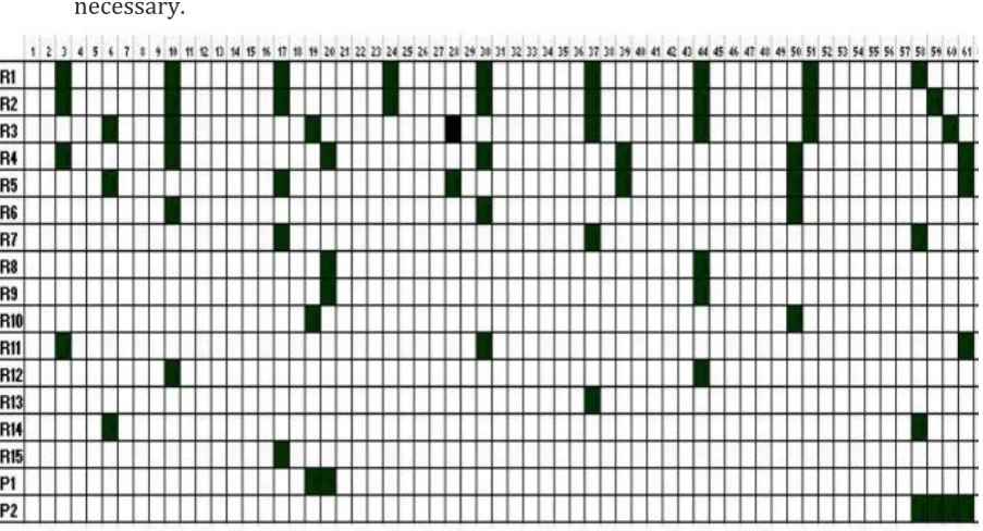
Preventive maintenance is planned in deterministic time slots (weeks) in a two-year period. The preventive maintenance they plan consist out of routine projects and undefined projects. Some routine works and projects may be combined to reduce the possession cost, but others may exclude each other. A list of projects that need to be performed in the planning period, duration and the earliest and latest possible starting times for each project are assumed known. Figure 7 is an example of a possible planning solution generated by (Budai et al., 2006))
The objective is to minimize track possession costs and the maintenance costs.
Overall cost = 𝑝𝑜𝑠𝑠𝑒𝑠𝑠𝑖𝑜𝑛 𝑐𝑜𝑠𝑡 + 𝑚𝑎𝑖𝑛𝑡𝑒𝑛𝑎𝑛𝑐𝑒 𝑐𝑜𝑠𝑡 + 𝑝𝑒𝑛𝑎𝑙𝑡𝑦 𝑐𝑜𝑠𝑡 (2. 1)
[19]
[image:20.595.73.525.153.397.2]loss of production, environmental damages or safety consequences (Budai-Balke, 2009). The Maintenance cost are assumed the same for each time slot within the planning horizon. The maintenance costs of each routine work and project and the costs of having a track possession in the planning period are assumed known. The penalty cost, are cost for executing routine maintenance before maintenance was necessary.
Figure 7 example of a maintenance schedule for 61 weeks containing 15 routine works (R1-R15 on Y-as) and 2 projects (P1 and P2 on Y-as) (Budai et al., 2006)
To escape local optimum, local search methods can be used. Within Memetic Algorithm and Iterative Heuristics, they looked at two local search methods: Simulated Annealing (SA) and Tabu-search. From these two Budai-Balke (2009) concluded that SA tended to give the best results in general. Out of 80 test instances, 49 times, SA gave a lower objective value than Tabu-search (TS). This leads to the conclusion that we will also use SA, as stochastic local search method.
Pouryousef et al. (2010) has created an extension to the model of (Budai-Balke, 2009). The following shortcoming in the model of Budai-Balke et al. is noted: the model is not sensitive to the simultaneous planning of several segments. Therefore, it might cause some
[20]
Jenema (2011) also looked at the minimization of track possession costs and the
maintenance costs. She has created an alteration to the PSMP, which is solved using branch-and-bound and the Gurobi solver. She used the segment system of (Pouryousef et al., 2010), but created an alteration on the possession sizes. These are the special features of her research:
A distinction is made between possession cost at night than during day.
The size of the possessions is depending on the maintenance activities that are planned in the possession. The different sizes of possession are predetermined.
Furthermore, a top 10 maintenance activities are determined that are influencing the possession planning in such a way that the top 10 could solely determine the
possession planning.This list is determined by an analysis on a benchmark on
realization data and discussion with experts. This list consists of routine maintenance activities, which can be performed between a minimum possession duration of 0,5 and 6 hours.
After the review of Lidén (2015) there are two more recent literature studies carried out, which we will discuss. The work of (Caetano & Teixeira, 2016) and (Pargar, 2015; Pargar et al., 2017)
Caetano & Teixeira (2016) have created a model to determine for each time slot whether renewal of ballast, rail and sleepers in different track sections of a bussable part of track will take place. As operational constraint of the model, it is assumed that the track component in each of the track segments is only renewed once during the planning time window.
Furthermore, the model also incorporates the decision to reuse railway track components from other tracks in renewal operations, to discount the maintenance cost. Finally, they also determine the number of maintenance activities for each track component k ∈ K during time
slot t ∈ T in each track segment n ∈ N of the bussable part of track. Same as in (Jenema,
2011) their model can select different possession types to perform the renewal operation. There nuisance cost is differently compared to the other researches, because the possession cost is not only dependent on possession time. With complete abstraction of the rail tracks they used the following calculation for nuisance:
𝑁𝑢𝑖𝑠𝑎𝑛𝑐𝑒 = ψ𝑑,𝑛,𝑏∗ 𝐸𝑇𝑀 * 𝑉𝑜𝑇𝑑 (2. 2)
𝑉𝑜𝑇𝑑=value of time (€) for each type of passenger with trip purpose d ∈ D, D is the
total number of trip purposes in which the value of time can vary.
ψ𝑑,𝑛,𝑏 = average number of passengers with trip purpose d ∈ D in track segment n ∈ N on bussable part of track b ∈ B during track possession;
𝐸𝑇𝑀 = expected increase in travel time for one passenger when other public
[21]
ProRail has developed a measurement methodology together with Locov and NS called extra amount of experienced travel time (ETM) to express experienced nuisance in minutes. This is different from the ETM of (Caetano & Teixeira, 2016), because it does not look at real increase travel times but at experience increase in travel time. An assumption of the model of ProRail is that all tracks are blocked by a maintenance possession. Furthermore, bus to bus transits are ignored. The formula created to calculate the 𝐸𝑇𝑀 value of one passenger is:
𝐸𝑇𝑀 = (𝑇𝑇 + 1,3 ∗ 𝐵𝑇 + 2 ∗ 𝑋𝑊𝑇 + 34 𝑋𝑂𝑇𝑇 + 43 𝑋𝑂𝐵𝑇) (2. 3)
𝑇𝑇 = average extra train time (min.) compared to the normal trip of one passenger
multiplied with percentage of people expected to take detour by train
𝐵𝑇 = bus time (min.) multiplied with percentage of people expected to take the bus 𝑋𝑊𝑇 = average extra amount of waiting time (min.) on bus or train.
𝑋𝑂𝑇𝑇 = average extra amount of transits train to train.
𝑋𝑂𝐵𝑇 = average extra amount of transits bus to train or train to bus.
The numbers 1,3; 2; 34 and 43 are based on research conducted by Schakenbos, Paix, Nijenstein, & Geurs (2016), they represented the experience time passengers experienced for the different variables. For example, one transit from train to train (XOTT), is equally experienced like traveling 34 minutes by train. For example, on a bussable part of track with three adjacent stations A, B and C. And there is a possession between A and B. The track is replaced by busses, the bus time is 15 minutes, and there is an average extra waiting time at station B between the bus and the train of 5 minutes. This leads to: 𝐸𝑇𝑀 = 72,5 =
(0 + (1,3 ∗ 15) + (2 ∗ 5) + (34 ∗ 0) + (43 ∗ 1))
Compared to equation 2.2, ProRail doesn’t include the VoT of different type of passengers. So, there is no difference in weight for a person who is traveling for work or leisure. This leads to the following equation for nuisance:
𝑛𝑢𝑖𝑠𝑎𝑛𝑐𝑒 = ψ𝑛,𝑏∗ 𝐸𝑇𝑀 (2. 4)
ψ𝑛,𝑏= average number of passengers on segment n, on bussable part of track b ∈ B
during the track possession.
In more recent work Pargar also worked on improving the PSMP model, by trying to find the right moment to renew a component instead of doing more preventive maintenance. The same structure of using different segments, like in (Pouryousef et al., 2010), is used. But there is also a reduction if work is planned in sequential track segments. A CPLEX solver is used to solve the model. He concludes that his model is too complex to use for large-sized real-life cases.
Objective function: minimizes the sum of possession cost, maintenance cost of performing maintenance or renewal and the cost of renting and installing the machines to perform renewal and maintenance.
Decide for each time slot for each component of each part of track one of the following actions: do nothing, do maintenance or do renewal.
[22]
2.2
Conclusion
We have identified different methods used for optimisation of a maintenance planning. What we have learned is that both exact methods as well as heuristics have been used in the past by researchers. In practice the problem could become too large to use an exact
approach. Therefore, a heuristic need to be created to find a solution. So far there is no research specifically on heuristics for the middle-to-long term rail infrastructure possession planning. Short term scheduling methods could be used, but need alterations due to the nature of the type of track work. As a framework we will use the work of (Budai-Balke, 2009; Budai et al., 2006). Our problem description is in many ways comparable to preventive maintenance scheduling problem (PMSP). We are also planning a given amount of work in each amount of deterministic time slots under certain constraints.Our solution has the same format as presented in their work, see Figure 7. Furthermore, we will use the alteration of Pouryousef et al. (2010) to simultaneous plan several segments. And same as Jenema (2011), different size possessions are accepted. Possession can have different properties compared to each other. But, there are four points that need alteration in our model compared to PMSP things that we will do different in our model are:
i) The type of maintenance ii) The Objective function
iii) Variable weight between cost and nuisance iv) Longer time window
In the next chapter, we will further explain these concepts and how this thesis will
[23]
3.
Problem modelling
This chapter consists of three parts. In the first part we will create a descriptive part explaining our model. Secondly, we illustrate our model by giving an example of its workings. In the third part of this chapter we willdefine the mathematical model. The mathematical model will include an objective function, parameter description and the constraints to which the model is subjected.
3.1
Model description
As explained in the conclusion of Chapter 2, there are some differences compared to the work on which we based our model (Budai-Balke, 2009; Budai et al., 2006). We will now create a descriptive part how our model will look like.
3.1.1 Assumptions
The following assumptions underpin the model developed in this chapter. It is assumed that for each possession the following items are known:
The cost for performing the possession in each year.
The deadline, before which year the possession needs to be performed.
The possessions that cannot be performed together on a bussable part of track. Furthermore:
There is no limit to the amount of possessions that can be planned in a year. All Possessions are independent.
The amount of experience nuisance can be based on an estimation for each bussable part of track, on the extra amount of travel time and number of passengers.
Opening the bussable part of track partly is negligible in relation to the amount nuisance reduction this will induce.
3.1.2 Type of maintenance
Our focus is on possessions larger than 4 hours, this can be different types of track works. The possessions are planned separately for each bussable part of track in the Netherlands. This is different compared to all the literate that is reviewed, which focusses mainly on routine maintenance. As explained in the section 1.2.1 Scope, on page 12, we are not looking at routine maintenance shorter than 4 hours. As such, we will not include any constraints on repeating possessions. We assume the possessions are independent of each other, and are only executed once in the time window. Therefore, we will not look at the sequence of possessions. There are possessions that can be performed simultaneously, we assume these are known. For our results we will create a list which possessions cannot be combined based on the track segment(s)8 needed of each possessions. If possessions are on the same
track segment we assume they cannot be combined.
[24]
3.1.3 Objective
Given a set of known possessions on one bussable part of track, which consist of multiple segments of track. The objective is to minimize the summed weighted nuisance and track work cost of the whole time window. We will now explain what measurement we will use for track work cost and nuisance.
Different from (Budai-Balke, 2009; Budai et al., 2006), but similar to (Pouryousef et al., 2010) and (Jenema, 2011), track work cost depend not only on the possession but also on the time slot in which the possession takes place. Now, there is no clear model at ProRail how the cost will change by shifting of possessions to another year. The main goal of this cost is to show that in the model it is possible to take different financial cost into account for different possessions over different years. To realize a model that is practical for ProRail, the following options should be included:
i) Different cost for different possessions ii) Change of cost over years
iii) Penalty cost
i) There are many different types of track works, so the cost for performing a possession can vary for different possessions. ii) In practice, cost can change over years by
postponing/advancing of possessions. iii) Penalty cost are also introduced, to model the more binary type of cost. By postponing the execution of a possession, ProRail might want to do to extra maintenance or it will induce extra risk. This extra maintenance or risk could be starting from a certain year and not a steady increase over years that is included in type ii). Any other type of penalty cost or financial could be easily implemented in our maintenance cost parameter, because this is a parameter. This financial cost model is just a proof of concept. The topic of creating a financial cost model could be further researched, to create a model that is closer to the practice at ProRail.
The nuisance for a possession, will be based on the research of ProRail and Caetano and Teixeira (2016). Based on Caetano and Teixeira (2016), a difference between the average people travelling during work days and weekend days a separation will be used to calculate the average number of passengers during a possession on a bussable part of track.
𝑃𝑤: Estimated number of passengers per hour on a bussable part of track during w ∈ {work day, weekend day}.
𝐷𝑤: Number of hours the possession takes during w ∈ {work day, weekend day}.
[25]
A formula is created to measure the amount of experienced nuisance of passengers:
𝑁𝑢𝑖𝑠𝑎𝑛𝑐𝑒 = ψ𝑏∗ (𝑋𝑅𝑏∗ (𝑈𝑏𝑢𝑠∗ 0,3 + 1)) (3. 2)
𝜓𝑑,𝑏: average number of passengers during a possession on bussable part of track b
∈ B; B all the bussable part of tracks in the Netherlands.
𝑋𝑅𝑏8: Estimated amount of extra time (min.) compared to the normal trip of one passenger. Simplified version of ETM.
𝑈𝑏𝑢𝑠9: Estimated percentage of passengers that travels with the bus.
This formula does not take the extra waiting time and extra transits into account. We think this is justified because in comparing a longer or shorter possession on the same part of track, you should have the same amount of transits and waiting time (when looking at a traveller who is travelling the complete bussable part). ETM is replaced by: 𝑋𝑅𝑏∗ (𝑈𝑏𝑢𝑠∗ 0,3 + 1). This contains an estimation, by ProRail, of the extra train time and extra bus time (𝑋𝑅𝑏) multiplied by the expected percentage travellers to travel by bus (𝑈𝑏𝑢𝑠) multiplied by
the factor that 0,3+1 (this is the extra weight for traveling by bus compared to train). So, if everyone would travel with the bus, 𝑈𝑏𝑢𝑠 = 1. This would lead to nuisance = ψ𝑑,𝑏∗ 1,3 ∗ 𝑋𝑅𝑏, such that all the extra time ((𝑋𝑅𝑏) is extra travel time by bus. Finally, we assume that if
there is a possession on a bussable part of track, the whole bussable part of track will be out of service.
3.1.4 Variable weight between cost and nuisance
In the literature reviewed so far nuisance cost and track work cost where compared without looking at the balance between the two factors. With one exception, in the work of (Caetano & Teixeira, 2016) where VoT is used from the work of (Wardman, 2004) Value of Time, is a measure of how much time of a passenger is worth. A downside of VoT is that a planning cannot be steered towards more/less nuisance/cost. In our model, we will use a factor 𝐾, to
compare nuisance with cost. So ProRail could use factor 𝐾 to create different solution
scenarios depending on whether cost or nuisance is more important. This leads to the objective value:
𝑂𝑏𝑗𝑒𝑐𝑡𝑖𝑣𝑒 𝑣𝑎𝑙𝑢𝑒 = 𝑐𝑜𝑠𝑡 ∗ 𝐾 + 𝑛𝑢𝑖𝑠𝑎𝑛𝑐𝑒 (3. 3)
3.1.5 Longer time window
The time window of our model is 5 years, as requested by ProRail. In practice not, all weeks of this time window are used to plan possessions. The number of time slots should be as low as possible, to reduce the computation time. To reduce the number of time slots in which a possession can be planned we use clusters.
A cluster represents a list which can be filled with possessions, the possessions that are on this list will be performed at the same time. If a possession is planned in a cluster, you know in which year it will be executed but not in which week. There can be multiple clusters in a
9𝑋𝑅
[26]
year. For the model, there are always equal number of clusters in each year, this makes it easier to create a solution method. It is possible in a year. Within a year, it is indifferent in which cluster a possession is planned for nuisance and cost. The number of clusters in a year is a predetermined number. But the number of clusters in a year can vary depending on the number of clusters necessary to find the optimum. A rule of thumb is presented in Chapter 5. If there is at least one empty cluster in each year, you can say for certain that you have enough clusters to find the optimum, when using an exact method. Increasing the number of clusters will also increase the solution space, as such it will take longer to find a solution for the heuristic. Therefore, a balance exists between computation time and good results.
3.2
Example of the model
An example will be used to show:i. How the list of possessions that cannot be clustered will be generated; ii. The amount of nuisance that is induced by individual possessions;
iii. The amount of nuisance reduction that is induced by clustering possessions. In this example three fictional possessions A, B and C on the bussable part of track between Den Haag HS and Rotterdam CS are used (Figure 8).
[image:27.595.76.520.297.547.2](A) (B) (C)
Figure 8 bussable part of track between Rotterdam Central and Den Haag HS, with three possessions A, B and C. The red part indicates on which track segments a possession will take place. (A) possession between Delft and Schiedam Centrum, (B) possession between Den Haag HS and Den Haag Moerwijk, (C) possession between Den Haag HS and Schiedam Centrum.
The parameters for calculating the amount of nuisance for this bussable part of track can be seen Table 3, and the parameters for the possessions, A, B and C, in Table 4. Now,
possessions are planned as much as possible in the weekend at ProRail, so we assume that if a possession is shorter or equal than 52 it will be fully performed in the weekend. It is possible to include different number of expected passengers for each year, for this example the amount of nuisance is kept steady over different years.
[27]
Table 3 estimated parameters for the bussable part of track between Den Haag HS and Rotterdam Central.
Variables Values
𝑋𝑅 30 min.
𝑈𝑏𝑢𝑠 25 %
𝑃𝑤𝑜𝑟𝑘 4,1 ∗ 103(
𝑃𝑎𝑠𝑠𝑒𝑛𝑔𝑒𝑟𝑠
𝐻𝑜𝑢𝑟𝑠 )
𝑃𝑤𝑒𝑒𝑘𝑒𝑛𝑑 2,2 ∗ 103 (
𝑃𝑎𝑠𝑠𝑒𝑛𝑔𝑒𝑟𝑠
𝐻𝑜𝑢𝑟𝑠 )
Table 4 nuisance and cost parameters for three fictional possessions A, B and C, displayed in Figure 8.
Possession Track segments
𝐷𝑤𝑜𝑟𝑘 (hours)
𝐷𝑤𝑒𝑒𝑘𝑒𝑛𝑑 (hours)
preferred execution
year
Deadline Cost 10 (euro)
A 2,3 0 52 2021 2023 5,00 × 10⁴
B 6 0 18 2023 2025 2,00 × 10⁶
C 2,3,4,5,6 0 52 2025 2027 2,00 × 10⁶
The list of combinable possessions in this thesis is generated based on the non-overlapping track segments of the possessions. Possession A and B have no non-overlapping track segments, as such we assume they can be clustered. Cluster A-C and B-C do have overlapping track segment; therefore, the list of non-combinable possessions consist of {A-C; B-C}.
Now we will show how the amount of nuisance for each possession can be calculated. Using equation 3.211, the amount of nuisance can be calculated for different planning solutions.
𝑁𝑢𝑖𝑠𝑎𝑛𝑐𝑒(𝐴 𝑜𝑟 𝐶) = 3,7 ∗ 107 (passengers ∗ minutes) = (0 + 52 ∗ 2,2 ∗ 103) ∗ (30 ∗ (0,25 ∗ 0,3 + 1))
𝑁𝑢𝑖𝑠𝑎𝑛𝑐𝑒(𝐵) = 2,0 ∗ 106 (passengers ∗ minutes)
= (0 + 18 ∗ 2,2 ∗ 103) ∗ (30 ∗ (0,25 ∗ 0,3 + 1))
10 Cost for performing the possession in the prefered performance year.
11𝐸𝑞. 3.2: 𝑁𝑢𝑖𝑠𝑎𝑛𝑐𝑒 = ψ
[28]
The combination A and B in the same cluster is not on the list of non-combinable possessions so it is possible to cluster possession A and B. This cluster will lead to the following amount of nuisance:
𝑛𝑢𝑖𝑠𝑎𝑛𝑐𝑒 = 3,7 ∗ 107 (passengers ∗ minutes)
= (0 + 52 ∗ 2,2 ∗ 103) ∗ (30 ∗ (0,25 ∗ 0,3 + 1))
The amount of nuisance reduction created by clustering possessions A and B is the complete amount of nuisance that would be induced by solely possession B. Because the whole
bussable part is out of service during a possession, 𝑁𝑢𝑖𝑠𝑎𝑛𝑐𝑒(𝐴 ∩ 𝐵) = 𝑁𝑢𝑖𝑠𝑎𝑛𝑐𝑒(𝐶). It does
not matter for nuisance that (𝐴 ∩ 𝐵) ≠ 𝐶, even though𝐴 ∩ 𝐵does not include the track
segment between Den Haag Moerwijk and Delft. As such, if possession A, B and C would have the same duration they would give the same amount of nuisance.
So far, in this example, we have calculated the amount of nuisance of each possession and the possible cluster. Finally, we will use this example to show how cost calculation will work. Steady increase of cost for advancing/postponing compared to the preferred year could for example be 3% over the cost of performing the possession (see Table 4) and a static penalty cost of € 1,00× 10⁶. In Table 5 we have calculated the cost for performing the three possessions A, B and C in different years, to show the steady increase and penalty works. Looking at possession A, the cost in 2021 are retrieved from Table 4 for performing the possession in the preferred year. Each year there is an increase of 3%, in 2024 and 2025 possession A is out of deadline (see Table 4) so a single penalty of € 1,00 × 10⁶ is required.
Table 5 Amount of cost for possessions A, B and C. In bold, the cost for performing the possession in the preferred year, using the parameters of Table 4.
Possession 2021 2022 2023 2024 2025
A € 5,00× 𝟏𝟎𝟒 € 5,15× 10⁴ € 5,30× 10⁴ € 1,05× 10⁶ € 1,05× 10⁶ B € 2,12× 10⁶ € 2,06× 10⁶ € 2,00× 𝟏𝟎𝟔 € 2,06× 10⁶ € 2,12× 10⁶ C € 2,25× 10⁶ € 2,19× 10⁶ € 2,12× 10⁶ € 2,06× 10⁶ € 2,00× 𝟏𝟎𝟔 In Table 6, we have calculated the total amount of nuisance and cost based on Table 5 for the scenario where we cluster A+B and the scenario were A and B are not clustered. There is a difference between these scenarios of: 𝑛𝑢𝑖𝑠𝑎𝑛𝑐𝑒 (𝑝𝑚) = −0,2 × 10⁶ and for
[29]
Table 6 two scenarios, were the cost are minimized based on Table 5, for the example: clustering A+B and not clustering A and B
Different scenarios can be generated based on factor K. Using equation (3. 3)this leads to:
𝑜𝑏𝑗𝑒𝑐𝑡𝑖𝑣𝑒 𝑑𝑖𝑓𝑓𝑒𝑟𝑒𝑛𝑐𝑒 = −0,2 × 10⁶+ 𝐾 ∗ 0,3 × 10⁴ (3. 4) So, for 𝐾 =2
3 × 10
2, the objective difference between clustering and not clustering would be 0. For 𝐾 <2
3 × 10
2 there is less weight on cost (so more on nuisance), as such leads to preference to cluster. For 𝐾 >2
3 × 10
2, there is more weight on cost (so less on nuisance) which as such leads to a preference of the model not to cluster.
In this example the optimum solution could be achieved using one cluster per year. If we would like to perform possessions A, B and C in the same year, multiple clusters are necessary in one year to achieve the minimum solution. Because there can be multiple clusters in one year the generated solution is not unique. For example, if the number of clusters in a year is two, cluster 1 and cluster 2 are of the first year. As such, cluster 1 and cluster 2 have the same nuisance and cost parameter. So, if possession A and B are in cluster 1 and possession C in cluster 2 this would result in the same objective value as putting possession C in cluster 1 and possession A and B in cluster 2. This explains how there can be different optimal solutions.
The amount of nuisance reduction can change depending on the clustering of possessions compared to doing possession individual. To reduce the number of decision variable in the model, we decided to calculate the amount of reduction in the following matter: by
combining two possessions, there is a reduction of the smallest amount of nuisance of the two individual possessions. The amount of reduction will be calculated based on
combinations in a cluster by taking the minimum value of the amount of nuisance of the two possessions.
1. Check if possession m and n are in set non-Comb. which contains all the possession combinations that are not allowed to be performed together, or m is equal to n 2. If so, 𝑛𝑑𝑡𝑚,𝑛 = 0
3. If not, 𝑛𝑑𝑡𝑚,𝑛= 𝑚𝑖𝑛(𝑛𝑡𝑚, 𝑛𝑡𝑛)
Possession
Clustering A+B Not clustering A + B
Execution
year Nuisance (pm) Cost minimized Execution year
Nuisance
(pm)
Cost minimized
A 2021 3,7 × 10⁷ € 2,00 × 10⁶
B 2023 2,0 × 10⁶ € 5,00 × 10⁴
C 2025 3,7 × 10⁷ € 2,00 × 10⁶ 2025 3,7 × 10⁷ € 2,00 × 10⁶ A+B 2023 3,7 × 10⁷ € 2,05 × 10⁶
[30]
To reduce the number of model variables we will not look correctly at the nuisance reduction. Because of this, there will be an overestimation of nuisance reduction than is valid. If more than two possessions are clustered. There is a reduction in decision variables, because we don’t look whether three (or more) possessions are combined in a cluster. This will help in the speed of solving the model using CPLEX. An example is used to show how the reduction is modelled: if there are three possessions, A, B and C in a cluster and the amount of nuisance of these possessions is n(A), n(B), n(C). The total amount of nuisance calculated by the model will be n(A)+n(B)+n(C)-min(n(A), n(B)) -min(n(A), n(C)) -min(n(B), n(C)). As such, there is one reduction term too much. The correct calculation would be: max(n(A), n(B), n(C)). In the results we will make an analysis of the effect of this overestimation.
3.3
Mathematical Formulation
Sets:
P contains a list with all the possessions that are on a bussable part of track.
𝑇 list containing the clusters in which a possession can be placed.
N the number of clusters in one year.
nonComb. {(m, n) | possession m is not combinable with n, ∀m, n ∈ P}. Decision variable:
𝑥𝑡𝑝 1 if possession 𝑝 ∈ 𝑃 is performed in cluster t ∈ 𝑇, 0 if it is not performed in
cluster t ∈ 𝑇. {0, 1}
𝑟𝑡𝑚,𝑛 gives a value 1 if possession m ∈ P and n ∈ P are in the same cluster t ∈ 𝑇.
{0,1}
Parameters:
𝐾 factor for to have a balance between finance and nuisance. Can be different
for each bussable part of track. (Euros per pm12)
𝑛𝑡𝑝 the amount of nuisance (pm) if possession 𝑝 ∈ 𝑃 is performed in cluster t ∈ 𝑇. 𝑛𝑑𝑡𝑚,𝑛 the amount of nuisance reduction (pm) possessions 𝑚 and 𝑛 ∈ 𝑃 give in
cluster t ∈ 𝑇, because possession m and n are combined. 𝑐𝑝𝑡𝑝 cost in euros for performing possession p ∈ P in cluster t ∈ 𝑇. 𝑀 is a large number compared to 𝑥𝑡𝑝, 𝑀 ≥ 2.
[31]
Objective function
𝑚𝑖𝑛 ∑ ∑
(
𝑥𝑡𝑝∗ (𝑛𝑡𝑝+ 𝐾 ∗ 𝑐𝑝𝑡𝑝) − ( ∑ 𝑟𝑡𝑝,𝑚∗ 𝑛𝑑𝑡𝑝,𝑚
𝑚∈𝑃 𝑚≠𝑝
)
)
𝑝∈𝑃 𝑡∈𝑇
(3. 5)
Subject to
∑𝑡∈𝑇 𝑥𝑡𝑝 = 1 ∀𝑝 (3. 6)
𝑥𝑡𝑚+ 𝑥𝑡𝑛 ≤ 1 ∀𝑡, (𝑚𝑛) ∈ non𝐶𝑜𝑚𝑏. (3. 7)
𝑥𝑡𝑚+ 𝑥𝑡𝑛− 1 ≤ 𝑀 ∗ 𝑟𝑡𝑚,𝑛 ∀𝑚, 𝑛, 𝑡 (3. 8)
2 − (𝑥𝑡𝑚+ 𝑥
𝑡𝑛 ) ≤ 𝑀 ∗ (1 − 𝑟𝑡
𝑚,𝑛)∀𝑚, 𝑛, 𝑡 (3. 9)
𝑟𝑡𝑚,𝑛, 𝑥𝑡𝑝= {0,1} ∀𝑚, 𝑛, 𝑡, 𝑝 (3. 10)
The objective function
The objective function consists of two parts. In the first part, it is stated whether a
possession is performed in a cluster. If so, how much nuisance and cost this will induce. The second part is a reduction of nuisance if two possessions are in the same cluster. 𝑛𝑑𝑡𝑝,𝑚 is the
amount of reduction if possession a and m are in the same cluster t indicated by decision variable 𝑃𝑡𝑝,𝑚. The amount of nuisance and cost are summed for each possession for each
cluster, were this objective value is calculated for one bussable part of track.
Constraints:
Constraint (3. 6) ensures that every possession is performed once in the time horizon. Constraint (3. 7) ensures that the combination of two possessions that are on the list non-Comb cannot be clustered.
Constraints (3. 8) and (3. 9) are responsible for the reduction of ETM if possessions are combined. When both possession m and n are in period t, then 𝑟𝑡𝑚,𝑛 will become 1. This will
give a reduction of 𝑛𝑑𝑡𝑚,𝑛 in the objective function.
Constraint (3. 10) makes the decision variables binary. A possession can either be, or not be assigned to a cluster.
Furthermore, it could be easily implemented that possession p is restricted of being performed in year t by adding the constraint 𝑥𝑡𝑝= 0. We assume that it is possible to
[32]
model. For example, for planning a possession after the deadline will induce a penalty cost could be included in parameter 𝑐𝑝𝑡𝑝.
3.4
Conclusion
In this chapter we created two descriptions of the model, a description in words and a mathematical formulation. Furthermore, we have given an example of the model, using three fictive possessions on the bussable part of track between Den Haag HS and Rotterdam CS. Compared to the preventive maintenance scheduling problem (PMSP) (Budai-Balke 2006), (Budai-Balke, 2009) there are four points that we altered in our model:
1. The type of maintenance
We will plan a set of known possessions longer than 4 hours on a bussable part of track. 2. Variable weight between cost and nuisance
Factor K can be used to influence the relation between experienced nuisance and financial cost. Therefore, it is possible for ProRail to create scenarios for the possession planning.
3. The Objective function
We minimize the objective function which is: over all possessions and clusters the summed amount of nuisance and factor K times the cost of a possession for performing the possession in cluster t.
4. Longer time window
We are working on a 5-year time window. Each year will have a predetermined number of clusters in which possessions can be performed, this will reduce the problem size compared to planning in every week.
[33]
4.
The solution method
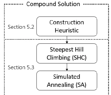
There are 96 unique bussable parts of track in the Netherlands. For each bussable part of track we need to determine which possessions to combine into clusters. To determine the optimal solution of small instances, solving methods such as branch and bound, dynamic programming (dip) and solving a Mixed Integer Linear Problem (MILP) with CPLEX can be used. The IBPIBM ILOG CPLEX Optimizer is used to solve the mathematical model described in Chapter 3 in MATLAB. Because the model is too large, for bussable part of tracks with lots of possessions, a heuristic can be used to find a solution. The question remains whether this solution is good enough. Our heuristics consist of a construction and an improvement step. In Section 4.1 we will explain what construction heuristics we will use and why. In Section 4.2 we will explain what improvement heuristic we will use. The goal of this chapter is to show the different possibilities for the construction and improvement step. Furthermore, explain how the heuristics work that are used. Finally, explain which component of the heuristic are investigated using numerical result in the next chapter.
4.1
Constructive heuristic
In the constructive heuristic an initial solution will be generated. In general, the constructive heuristic can be described as:
Define the possessions that aren’t assigned to a cluster yet; 1. Use a selection method to select a possession from step 1; 2. Assign the possession to a cluster;
3. Repeat step 1-3 until all possessions are assigned to a cluster.
The possession can be selected and assigned deterministic or probabilistic, these are two different type of construction heuristics. Considering the consistency of deterministic
heuristics, we will use a greedy approach as a candidate construction heuristic. We leave out probabilistic construction methods, because we will already be using a probabilistic
improvement heuristic. A downside of greedy construction methods is that they are not designed to escape local optimum. The global optimum is always a local optimum. As such, there is a chance that the local optimum found by the greedy approach is the global
optimum. An example is shown in Figure 9, where in the red area (a smaller solution space), L would be the local optimum (minimisation). In Figure 9, G is the global optimum. A greedy method could get stuck in the local minimum L, while there is are better solution G.
[34]
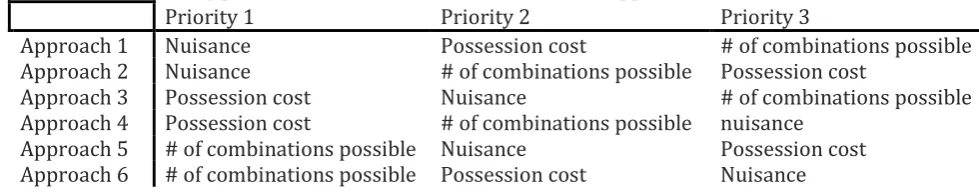
Greedy approach is a deterministic approach in which at every step, one possession is added to a cluster in the order of a priority list. The priority list consists of every possession sorted following a priority rule. Possessions are assigned to the cluster that gives the lowest
objective value. Three parameters which have a high influence on the objective function are selected for the priority rule:
i) Duration (decr.) ii) Cost (decr.)
iii) Combinations possible (incr.)
Same as (Budai-Balke, 2009) possessions will be sorted from largest duration to smallest duration, because longer possessions will induce more nuisance. Also by combining
possession with a longer duration a higher reduction of nuisance could be achieved. There is a higher reduction of nuisance in combining two large possessions, compared to combining a smaller possession to a large possession or compared to combining two small possessions. Furthermore, cost also has a direct influence on the objective function. The cost is
determined by the year in which possessions are executed. So, to perform costlier possessions not in the preferred year is more expensive compared to less expensive possessions. Finally, amount of combinations possible also has an indirect impact on the objective function. The amount of combinations possible, can be determined by counting the amount of times the possession occurs on the list non-Comb. which is assumed known. The last possessions that will be clustered in the construction heuristic, will have less
possibilities to be placed in clusters. When there are less possibilities to place a possession with another possession, there is a lower chance that it can still be clustered. If possessions cannot be clustered this could lead to a lower reduction of nuisance. Beforehand, it is difficult to say which prioritising will give the lowest objective value therefore we will test different orders with the three parameters described above.
To conclude, the deterministic construction method we will be testing is:
1. Sort all the possessions in the order of Table 7, were priority 2 and 3 are tie breakers. 2. Pick the highest possession in the sorted list that hasn’t been planned.
3. Place the possession in a cluster that will give the lowest objective value that is feasible.
a. If there are equal objective values for different clusters, place the possession in the first possible cluster.
[image:35.595.67.557.659.757.2]4. Repeat step 2 and 3 until all possessions are planned.
Table 7 Sorting priorities for the deterministic construction approaches.
Priority 1 Priority 2 Priority 3
Approach 1 Nuisance Possession cost # of combinations possible
Approach 2 Nuisance # of combinations possible Possession cost
Approach 3 Possession cost Nuisance # of combinations possible
Approach 4 Possession cost # of combinations possible nuisance
Approach 5 # of combinations possible Nuisance Possession cost
[35]
4.2
Improvement heuristic
Improvement heuristic are used to improve an initial solution which is generated with a constructive heuristic, which are keen to get stuck in local optimum. Examples of
improvement algorithms are steepest hill climbing (SHC), r-opt, Or-opt, Simulated Annealing (SA), Tabu-search (TS), Genetic Algorithm (GA), Memetic Algorithm (MA), Iterative
Heuristics (IH). We would like to test both the results of a deterministic and stochastic improvement heuristic, to determine what type is probably most effective. Considering the results of Budai-Balke et al. (2006), as explained in chapter 3, we will use SA as stochastic improvement heuristic. GA, MA and IH are left out due to the larger computation time compared to SA. Note, we don’t think these are not useful for this problem, and could be considered in future research. Same as Budai-Balke et al. (2006), Steepest hill climbing (SHC) will be used as deterministic improvement heuristic.
In this section we will first explain how SHC and SA work. Secondly, we will explain what neighbourhoods are considered in this research.
4.2.1 Steepest Hill Climbing (SHC) and Simulated Annealing (SA)
i) Steepest hill climbing:
Looking at all the neighbours in a neighbourhood, and select the neighbour that will give the lowest objective function. Repeat this step until no neighbours give a lower objective
function.
1. Start with an initial solution.
2. Construct a neighbourhood, using one of the methods explained in Section 4.2.2. 3. Select the neighbour that gives the lowest objective value.
4. Repeat step 2-3 until the objective values stops decreasing.
ii) SA
The Simulated Annealing algorithm is based on the amount of movement particles have when cooling down. With high temperature, there is fast movement and with lower temperature, there is slower movement. In simulate annealing, the temperature is slowly lowered. The temperature indicates the percentage that a bad neighbour solution is accepted. In the beginning, when the temperature is high, (almost) all neighbour solutions are accepted. When reaching lower temperatures, (almost) only better solutions are accepted. This is designed to help escape local optimum.
1. Start with an initial solution.
2. Construct a neighbour solution, using one of the methods explained in Section 4.2.2 3. Compute the difference in objective value between the current solution and the
constructed neighbour solution.