Estimating lead time using Markov Chains

Estimating lead time using Markov Chains

Master of Science Applied Mathematics

Operations Research

University of Twente, Enschede, the Netherlands

PUBLIC VERSION

Due to confidentiality, some information is left out of this public version. Deleted parts are replaced byCONFIDENTIAL and the measurament unit of the lead time has been

replaced with ”unit”.

Student number 1583107

E-mail [email protected]

Project duration 4th of June 2016 - 10th of February 2017 Supervisors

Dr. J.C.W. van Ommeren University of Twente

PDEng M. Goldak Vanderlande Industries B.V. Graduation committee

Dr. J.C.W. van Ommeren University of Twente Prof.dr. R.J. Boucherie University of Twente Dr. B. Manthey University of Twente

Abstract

The goal of this thesis is to create a prediction model that can estimate the lead time of LFL (Load Forming Logic), a software product of Vanderlande Industries B.V. The research started by investigating order data, such as weight and volume, and continued with a series of

regression, ensemble and Markov chains models.

Preface

Since I was in primary school I wondered why we study mathematics. How are trigonometric functions going to help me in the future. For some reason, I enjoyed calculus classes. But, I never thought that mathematics would mean so much for my future education and job. Writing this thesis at Vanderlande Industries B.V., in such a great environment, with professionals with mathematical backgrounds, made me understand how applicable mathematics is in everyday life. My assignment was very practical and I learned a lot in this period.

Contents

1 Introduction 1

1 Problem identification and motivation . . . 1

2 Research goal . . . 1

3 Approach . . . 1

4 Report structure . . . 2

2 Background 3 1 About Vanderlande Industries B.V. . . 3

2 Load Forming Logic . . . 3

2.1 Order and recipe . . . 4

2.2 Carriers . . . 4

2.3 Arhitecture . . . 5

3 Literature review 7 1 Regression . . . 7

1.1 Ridge and Lasso . . . 7

1.2 Elastic Net Regression . . . 8

2 Ensemble methods . . . 8

2.1 Bagging method . . . 8

2.2 Boosting method . . . 9

3 Markov chains . . . 9

4 Clustering . . . 10

5 Performance measurements . . . 10

4 Data 11 1 Data analysis . . . 11

5 Prediction models 13 1 Regression models . . . 13

1.1 Assumptions . . . 13

1.2 Performance . . . 14

1.3 Elastic Net Regression - Approach . . . 14

1.4 Elastic Net Regression - Results . . . 15

2 Ensemble methods . . . 15

3 Confidence intervals . . . 16

6 Markov chains 18 1 Context . . . 18

2 Approach . . . 18

3 First results . . . 21

4 Confidence Intervals . . . 21

5.1 Clustering . . . 22

5.2 Regression . . . 23

7 Sensitivity Analysis 25 1 Altering data and model’s specifications . . . 25

2 Configuration parameters . . . 26

8 Conclusions and recommendations 28 9 Glosarry 30 10 Bibliography 31 Appendices 32 A Features set . . . 33

B Regression assumptions . . . 34

C Influential features . . . 36

D Confidence Intervals . . . 37

E Clustering Analysis . . . 40

Chapter 1

Introduction

This chapter discusses the problem to be investigated, motivation, the approach and summarizes the structure of this paper.

1

Problem identification and motivation

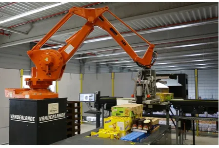
Automated Case Picking (ACP), a product of Vanderlande Industries, deals with automated order picking systems. Load Forming Logic (LFL) software product is the principal component of the ACP system.

LFL software receives as input an order from a store and its goal is to find a way to stack it in as less carriers as possible, while keeping the stacks stable. LFL’s ouput is called a recipe. Currently, LFL does not know, when it receives an order, how much time it will take to solve staking the order (to compute a recipe); thus, thelead time of the order is unknown in advance. Being able to predict this lead time will bring Vanderlande 2 major benefits:

1. It will indicate the number of necessary hardware components: LFL is a computationally expensive software and it is designed to run across many CPU cores and clusters of computers. Knowing the lead time of the orders can help to determine the number of necessary hardware components

2. Improve planning and scheduling of orders over the existing hardware components

2

Research goal

The end goal of the research is to create a prediction model that can estimate the lead time of the orders. This estimation can be based upon the characteristics of an order - called order profile. These order profiles and the resulting LFL lead time are used for training the models. This LFL software is used by three major clients worldwide, and each customer uses different carrier types, products assortment, and number of requested products. As several versions and configuration parameters of LFL can have a wide range of lead times for the same order, the prediction model has to be trained with a specific version and configuration prameters of LFL in mind. However, this model should be flexible and support various versions and configuration parameters.

3

Approach

ˆ Regression: ridge, lasso and elastic net ˆ Ensemble methods: bagging and boosting

In addition, we tried to model LFL’s architecture and behavior with Markov chains. For different configurations of LFL, the final models are re-trained, so that we test the influence of these changes in their performance.

In the end 2 models are compared: elastic net regression and Markov chains. Thebest one is recommended to be used for the prediction of lead times, along with pros and cons.

4

Report structure

The rest of the work is structured as follow:

ˆ context of the problem (Chapter 2) focused on describing the architecture of Load Forming Logic, the parameters of the software and characteristics of an order;

ˆ literature review (Chapter 3) describes the methods used in the research, together with the metrics used for measuring the performance of the models;

ˆ data (Chapter 4) contains the data analysis and construction of the features used for the regression models;

ˆ investigated models (Chapters 5 and 6), explain the approach and results of the regression, ensemble and Markov chain models;

ˆ sensitivity analysis (Chapter 7) summarizes the influence of small changes in data and parameters on the models performance;

Chapter 2

Background

This chapter focuses on describing the context of the analysed problem, the arhitecture and processes of LFL.

1

About Vanderlande Industries B.V.

Vanderlande Industries B.V. provides automated material handling systems and services that focus on improving customers’ logistics processes and increasing their logistics performance through out the entire life cycle. Automated Case Picking (ACP) is one of such systems. ACP enables fully automated order picking of a wide variety of products. It provides the answer to the most important challenges of today’s retail distribution. At the heart of this system lies a component Load Forming Logic (LFL), which is responsible for planning how an order is handled.

2

Load Forming Logic

LFL is a standalone module, which takes an order as an input and produces a recipe. This software is responsible for answering the questions:

2.1 Order and recipe

An order consists of a list of products together with the quantity of each product. For example, if there are 10 products X (e.g. box of chocolates), it means that there are 10 cases of chocolate. The cases of an order are diverse and:

ˆ have different dimensions, weight and volume ˆ have bottom and/or vertical rigid or not

ˆ belong to different groups. For a customer it is important that, for example, a carrier contains only products that belong to the same or similar group (e.g. cheese, milk, yogurt) because in shops they belong in the same alley, maybe on the same shelf.

ˆ have different support types: can support weight on the entire top surface, or only on the mid, corners or sides.

Figure 2.1: Example - support types for cases

ˆ have different forms; for example, there are cases containing PET bottles which usually are not dense and these cases cannot support many other cases on top of them

All these properties are taken into account while trying to build a stable stack.

The output of LFL, the recipe, is sent further to the palletizer which builds the stacks. Thus, a recipe contains not only the products assigned to each carrier and their position, but also the order in which the products have to be picked up (stacking sequence) from the deposit shelves and arranged on the carriers.

Figure 2.2: Palletizer

2.2 Carriers

fill rates can be changed by the software in some special cases, for example the maximum fill rates can lowered when LFL registers no progress while trying to stack the order.

Figure 2.3: Types of carriers

2.3 Arhitecture

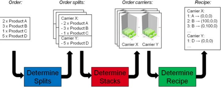
The architecture of LFL is complex: the software divides the problem into small processes which use different algorithms to solve them. LFL consists of 4 components: blue, red, green, and purple. The first three components communicate with each other through the purple component, which outputs the recipe at the end.

Figure 2.4: Load Forming Logic design

Flow of LFL is:

1. The process starts in the blue component: an order (multiple cases) enters the component where it is distributed over carriers. There are more ways to split an order, and the order split, which has the best score in terms of some established KPI’s, is chosen

3. The stacks that are considered stable and complete are sent further to the green com-ponent. This determines the sequences and robot movements for arranging the products on the carriers. The stacks that were not considered stable go back to purple component (next iteration starts) which is sending them again to blue, red and green component.

4. The process stops when all stacks are stable, and so a recipe was produced

The time it takes since an order enters LFL and until a recipe is produces is called the lead time of an order. Estimating the lead time of an order is the goal of this thesis.

Chapter 3

Literature review

This chapter covers all methods and models used in this research: regression methods (ridge, lasso and elastic net), ensemble methods (bagging and boosting), decision trees and clustering, Markov chain and performance measurements.

1

Regression

Regression is one of the most common method used in statistical analysis and predictions. It is a technique focused on the relationship between a dependent (response) and independent variables (predictors).

Ordinary least squares (OLS) is the most used method for estimating the coefficients of the independent variables by minimizing the residual squared error. For multi-linear regression the estimates of the coefficients β are obtained by solving equation 3.1.

βmultilinear= arg min β

X

(Y −βX)2 (3.1)

Where:

ˆ β - is an n dimensional vector of coefficients for all independent variables ( β1, β2, ...βn)

ˆ X -is an mxnmatrix corresponding to n independent variables and m observations ˆ Y - is an m dimensional vector of dependent variable for the observations (Y1, Y2, ...Ym)

For such a method to give good and relevant results, some assumptions have to be checked: linearity, homoscedascity, normality and multicollinearity. Linearity means that the relationship between the independent variables and the dependent variables is linear. Homoscedasticity suggests that the variance of residuals (difference between observed and predicted value) is the same for any value of the independent variables. Data presents normality if for any fixed value of an independent variable, the dependent variable is normally distributed. Multicollinearity occurs when the independent variables are dependent on each other.

1.1 Ridge and Lasso

Ridge regressionis a method used when data suffers from multicolinearity. It achieves better predictions compared to multi-liear regression ([2],[3],[4]) through a bias-variance trade off (*add more). It solves the multicolinearity problem through shrinkage of coefficientsβridge, using the

λparameter in 3.2

βridge= arg min β

X

The second term, theL2norm ofβ, is called a penalty because its role is to shrink the coefficients (β) with the final goal of having a low variance.

Lasso regression follows the idea of regularization, just as ridge regression. βlasso= arg min

β

X

(Y −βX)2+λX|β| (3.3)

The difference, compared to Ridge, is that the Lasso ([5]) can set some coefficients to 0. This is done by the penalty, L1 norm of β, which again controls the amount of shrinkage of the coefficients. As λ increases the coefficients shrink to 0; this way, the method performs as a variable selection model. But this method has also some limitations ([6]) e.g. if there is a subset of variables for which the pairwise correlations is high, Lasso tends to select only one variable from this subset (and it does not care which one). Elastic net regression solves this limitation.

1.2 Elastic Net Regression

Elastic net was proposed as a combination between Ridge and Lasso regression. Similar to Lasso, it performs automatic variable selection and continuous shrinkage ([7]), but the difference is that it can select groups of correlated variables. This procedure (3.4) is recommended when there are independent variables which are correlated. Lasso is likely to pick one of these at random, while Elastic net is likely to pick a group from them. L2 norm (used in Ridge regression) encourages parameters’ shrinkage with the final goal to have very low variance.

β= arg min

β

1 2N

X

(Y −β0−βX)2+αkβk21+ 1−α

2 kβk 2

2 (3.4)

Here, α is a positive regularization parameter, which for values in interval (0,1), the penalty interpolates between the L1 and L2 norm.

2

Ensemble methods

Ensemble methods use multiple learning algorithms to obtain better predictive performance ([8]) that could be obtained from any of the learning algorithms alone. Usually, ensemble techniques (especially bagging) tend to reduce problems related to over-fitting of the training data.

2.1 Bagging method

Bagging method can be used in combination with any kind of prediction model. The main idea of this method ([9]) is: giving a training set of sizen, there are generatedm bootstrap samples (samples with replacement) each of size n0, and each of these m samples are fitted with the chosen model. The output is the average of allm results.

In this paper, bagging is used in combination with elastic net and decision trees. Decision trees are usually constructed using CART (Classification And Regression Tree). CART starts searching for every distinct values of all its predictors (indipendent variables), and splits the value of a predictor by minimizing 3.5.

SSE = X

i∈S1

(yi−y¯1) + X

i∈S2

(yi−y¯2) (3.5)

Where ¯y1 and ¯y2 are the average values of the dependent variable in groupsS1 andS2 and yi is

from all the predictors (features), the one that splits better the data at that node. Bagging in combination with decision trees, improves variance by averaging the outcome from multiple fully grown trees on variants of the training set.

2.2 Boosting method

Boosting([10],[11]) method follows 2 steps: first, uses subsets of the original data to produce a series of averagely performing models and then, second step, it ”boosts” their performance by combining them together using a particular cost function (a majority vote). Unlike bagging ([12]), in the classical boosting, the subset creation is not random and depends upon the perfor-mance of the previous models: every new subsets contains the elements that were (likely to be) misclassified by previous models. Boosting is calling a “weak” or “base” algorithm many times, each time trained on a different subset (each subset has different weighting over the training examples). Every time the ”weak” algorithm is called, it generates a new weak prediction rule and after many iterations, the boosting algorithm, must combine these weak rules into one single prediction rule.

Least square Boosting fits consecutive trees, where each solves the net error of the prior trees (trees are dependent). Thus each new tree is fixing up the differences of entire system.

3

Markov chains

Many times, Markov chains can be used as a tool in decision making models ([13]) or in appli-cations of optimization, statistics and economics ([14]). What we try to do, is to use them as a tool in a prediction model. The definition of Markov chains is:

Let {Xn, n= 0,1,2, ...} be a sequence of random variables which takes values in a discrete

state space S. This sequence is aMarkov chain if

P{Xn=sn|Xn−1 =sn−1, Xn−2 =sn−2, ...X0=s0}=P{Xn=sn|Xn−1 =sn−1} (3.6)

for n ≥ 1 and sk ∈ S,0 ≤ k ≤ n. We assume that Markov chain is stationary i.e. the

probabilities P{Xn = s|Xn−1 = s0} do not depend on n. We refer to this probability as the transition probabilitypij. In a Markov chain, the system moves from one state to another with

a certain probability.

Figure 3.1 is an example of a Markov chain with 2 states, with the possibility to move from one state to another, possibly same state, with the respective transition probabilities. In the proposed model of this paper, there is a cost assigned to each transition.

In conclusion, a Markov Chain is defined by a set of state,S={s1, s2, s3, ...}with transition probabilities: P = {pij}. To predict the lead time, we will also assign a duration to each

transition C={cij}

4

Clustering

K-means clustering is a method of cluster analysis. The goal as discussed in [15] and [16] is to group the data based on their similarities. The algorithm works iteratively to assign each data point to a cluster, by minimizing the sum of distances from a point to the center gravity (centriod) of a cluster. Its output are the centroids of the k clusters (used to label new data) and the labels for the training set.

Giving a set of observations (x1, x2, .., xn) the goal of the method is to group the n

observa-tions into k clusters C ={C1, C2, .., CK}, while minimizing the within-cluster sum of squared.

Thus find the clusters which fulfill:

arg min C k X i=1 X

x∈Ci

||x−µi||2 (3.7)

whereµi is the mean of data inCi.

5

Performance measurements

For determining the quality of the predictions and also for comparing different methods, a set of performance measuraments ([17],[18]) are used:

1. MAE - Mean absolute error measures the average absolute differences between the observed and predicted values. It takes nonnegative values and values closer to zero indicate a good performance. Formula: M AE = _m1 Pm

i=1(yi−yˆi).

2. STDev - Standard deviation for absolute errors measures the standard devia-tion of absolute differences between the observed and predicted values. It also takes nonnegative values and values closer to zero indicate a good performance. Formula: ST Dev=»_m1₋₁Pm

i=1|(yi−yˆi)−M AE|2.

3. MRE - Mean relative error measures the average relative differences between the observed and predicted values and it can take any value. Values closer to zero indicate a good prediction; positive number suggest over-estimation and negative number under-estimation. Formula: M RE = _m1 Pm

i=1(yyˆii −1).

Notations used:

ˆ yi - observed value

ˆ yˆi - predicted value

ˆ y¯i - average of observed values

ˆ m - number of observations

Chapter 4

Data

This chapter discusses what type of data was used in the research and includes an analysis focused on data characteristics. The data set is extracted from the input of LFL software (section 2.1) and it contains the characteristics of the orders.

As LFL is in development, Vanderlande Industries collects data from the three customers for development and testing purposes. Thus, 3 sets of orders were provided for the research. The references for the customers are going to be: CU ST1,CU ST2 andCU ST3. Data sets have been split into training and testing data in percetages of 70% and 30% respectively, for all tested models. The samples have been extracted randomly.

CU ST1 CU ST2 CU ST3

550 orders 291 orders 70 orders

Table 4.1: Data sets

Each data example consists of a set of features that describe an order: volume, weight, number of products etc. The features (Appendix A) are these characteristics from LFL’ input plus other derived features, such as number of products which have full support type, or ratio of the ’light’ products etc. In total we destinguish 56 features.

1

Data analysis

To give an idea about the orders, some basic statistics are computed. As shown next, orders from the first two customers seem to be more complex and this can lead to a larger lead time. The third customer has smaller orders, from the point of view of weight, volume, and it does not contain ’bad’ cases (Appendix A).

CONFIDENTIAL

LFL needed, on average, more time to complete orders fromCU ST1andCU ST2,CONFIDENTIAL , and aroundCONFIDENTIAL forCU ST3.

CONFIDENTIAL

The lead time seems to be correlated (Figure ??) to the number of cases of an order (as there are more cases, the lead time increases) and also to the number of initial suborders (a suborder corresponds to a part of an order, which can fit volume and weight wise in a carrier).

For some orders from the third customer, LFL needs less than CONFIDENTIAL to process them (even if the number of cases varies from 1 to 600) which indicates that this feature is not correlated to the lead time. Thus, the increase in the lead time is not necessarily determined by the number of cases. Nevertheless, the number of initial suborders is positively correlatedt to the lead time.

Chapter 5

Prediction models

Chapter 5 presents several prediction models that have been tested, in order to find the best performing model. It turns out, that elastic net regression has the best results. In total, 3 regression models (lasso, ridge and elastic net) and 2 ensemble methods (bagging and boosting) were tested. The performances of all methods, for data set of CU ST1, are presented and the performance of Elastic net regression, for all 3 data sets. Only data set of CU ST1 was considered because for all methods, as shown next, it was the only set which fully met the required assumptions for regression models.

1

Regression models

Ridge, lasso and elastic net are multi-linear regression models with regularization. Depending on the method, they penalize the non-influential features (decrease their coefficients) or even perform variable selection (set the coefficients to zero).

1.1 Assumptions

The 4 assumptions, namely linearity, homoscedascity, normality and multicolinearity, have been checked in order to have relevant results of regression models: linearity, homoscedascity, normality and multicolinearity. The multicolinearity assumption is not a mandatory assumption for all regression models, since they are recommended to be used for multicolinear data.

The linearity property states that the relationship between the dependent variable (the lead time) and independent variables ( 56 features) has to be linear. The data set for CU ST1 presents linearity while the other 2 data sets do not: the plots Residuals vs Fitted (Appendix A) do not suggest any clear nonlinear model, thus a linear one may do as well as any other, and also, it has the virtue of simplicity. Having the same variance of residuals as for any of the independent variables suggesthomosceascity, meaninig that data should have little or no autocorrelation. Using Durbin Watson test (Appendix A) and analysing again the Residuals vs Fitted plots, it has been proven that data set for CU ST1 presents homoscedascity, while the other 2 sets do not (the plots show nonconstant variance in data). The consequence of the latter sets, heteroscedascity, usually results in confidence intervals that are too wide or too narrow and it may give too much weight to a small subset of data when estimating coefficients. The third property, normality, investigates if for any fixed value of an independent variable, the dependent variable is normaly distributed. All 3 data sets present normality, assumption checked byQ-Q plots of the residuals (Appendix A) (points should follow the diagonal line in order to be normal).

(for all data sets), the independent variables (the features) are not strongly correlated (correla-tion less than 0.5) but there are some features which are actually strongly correlated (correla(correla-tion greater than 0.8). Further, it will not be a problem, since the regression types that are going to be used are suited for correlated data and they solve this issue.

1.2 Performance

Regression models were run using lasso function implemented by Matlab®Software Statistics Toolbox (Release 2016a; The MathWorks Inc.) with 10-fold cross validation. Parameter α of the function, has been set to 1, 0.5 and 0.0001 for Lasso, Elastic Net and Ridge regression respectively.

The models can be compared by analysing the mean absolute error which should be correlated to a small standard deviation of the absolute errors. Large standard deviation together with small mean absolute error can suggest bad perfomance and large errors. Also, a small value of mean relative error (which compares the errors to the value of the real lead time) means the errors are a small proportion of the lead time.

Metrics Elastic net Ridge Lasso

Train data Test data Train data Test data Train data Test data

MAE 2.8059 2.5056 4.0910 3.4812 3.2952 2.6172 STDev 2.9424 2.1793 3.8201 2.3702 3.9364 2.0869

MRE 11% 3% 19% 22% 7% 7%

Table 5.1: Performance - regression models- CU ST1

Table 5.1 clearly indicates elastic net regression as the best model. Mean absolue error is 1-2 units and MRE is 11% and 3%, for training and testing data, respectively.

1.3 Elastic Net Regression - Approach

Before running any regression model, the data has to be standardized (because of different unit measurement of the features). There are 56 independent variables (set of features) and one dependent variable (the lead time). For all these variables, their z-scores have to be computed and these values are used in the model. A z-score is the standardized value of the initial value and is computed after the next formula.

For orderx and feature i, the z-score is:

zscoref eaturex,i =

f eaturex,i−meanf eaturei

standardDeviationf eaturei

(5.1)

Elastic net regression is trying to find the best coefficients for the features after the formula:

β= arg min

β

1 2N

X

(Y −β0−βX)2+αkβk2+ 1−α

2 kβk 2

2 (5.2)

1.4 Elastic Net Regression - Results

Elastic net regression was run for each customer (data set) separately. As a result, for each customer, different features with different weights were selected: 13, 11 and 7 selected features forCU ST1,CU ST2 and CU ST3, respectively (Appendix C).

Elastic net regression was performed 2 times: in the first run, the raw data is used as input and represents a variable selection method, whereas in the second run, we use the output of the first run as input. For example, for CU ST1, Elastic net regression selects 14 features in the first run and after the second run, one feature is excluded. The output of the later run are the coefficients of the variables, which are slightly different compared to the coefficients from the first run. Also, MAE improved with approximately 1 unite and the other metrics slightly decreased, as well.

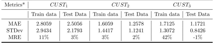
For CU ST1, the lead time of an order is mostly influenced by CONFIDENTIAL. The averageabsolute error is less than3units with a standard deviation of the absolute errors of also 3 units. Also, the mean relative error is quite small for the testing data (3%) compared to the training data (11%).

For CU ST2, the lead time of an order is mostly influenced by CONFIDENTIAL. The averageabsolute erroris1.5units with a standard deviation of the absolute errors of around 1.2 units. Again, the mean absolute error is small, only 2-3%.

For CU ST3, the lead time of an order is mostly influenced by CONFIDENTIAL. The averageabsolute erroris of 2 units with a standard deviation of the absolute errors of 1 unit. Nevertheless, the mean relative error is large: 42% for the training data (the model overpredicts) but small for the testing data (-1%). *All metrics are described in Section 3.3

Metrics* CU ST1 CU ST2 CU ST3

Train data Test Data Train data Test Data Train data Test Data

MAE 2.8059 2.5056 1.6059 1.2578 1.7125 1.1721 STDev 2.9434 2.1793 1.4417 1.1241 1.3072 0.8426

MRE 11% 3% 3% 2% 42% -1%

Table 5.2: Prediction performance - Elastic Net

2

Ensemble methods

In our investigation were performed both the bagging and boosting method.

Bagging method can be used in combination with any kind of prediction model; in this case, elastic net regression and decision trees were chosen. 50 bootstrap samples ([9]) were extracted, each of 250 orders; for each sample, a prediction model was run. In the end, the final predicted lead time is the average of the 50 predicted lead times of each sample.

Metrics Bagging & elastic net Bagging & decision trees Train data Test data Train data Test data

MAE 4.5869 4.7793 2.0611 3.7869 STDev 4.4163 4.5753 2.4656 3.4497

MRE 58% 89% 21% 51%

Table 5.3: Performance - Bagging-CU ST1

Wrapping up, bagging method performes better having as a ”weak” learner the decision trees instead of elastic net regression. Nevertheless, even if the MAE is small (with decision trees as ”week” learner), MRE is of 51% for testing data.

Further, the boosting method called Least Square Boosting was tested (predetermined func-tion fitensemble) with the following parameters:

ˆ method: ’LSBoost’

ˆ ”weak” learner: decision trees (constructed with function templateTree with 8 maximal number of decision splits (or branch nodes) per tree)

ˆ learning cycles: 30 (number of times of training the ”weak” learner)

ˆ learning rate: 0.1 (controls the contribution of the weak learners in the final combination)

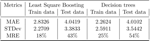
We also tested the performance of using only decision trees (fitrtree with 8 maximal number of decision splits and with other parameters default values) but neither of the last 2 models, performed better than Elastic net regression. Their results show MAE of around 3-4 units and MRE between 20% and 50%.

Metrics Least Square Boosting Decision trees Train data Test data Train data Test data

MAE 2.8326 4.0419 2.2624 4.0102 STDev 2.2709 3.3833 2.5911 3.5442

MRE 18% 43% 25% 54%

Table 5.4: Performance - Boosting and Decision Trees- CU ST1

In conclusion, Elastic net has the best performance from all the methods discussed above.

3

Confidence intervals

In general, for regression models, it can be verified how much influence the data set has on the results, by computing the confidence intervals for the selected features. These bounds were checked for all 3 data sets (customers) - Appendix D. Using the lower and then the upper bounds of the coeffients, Elastic net was performed again in order to see their effect on the lead time.

10-14% , 50-90% and decreased with 50% respectively.

Using the upper bound of the coefficients as weight in Elastic net, leads into a very small improvement in the performance for CU ST1, but for the other 2 customers, performance de-creases with a very big difference regarding mean relative error 50-90%.

Chapter 6

Markov chains

This chapter focuses on describing how Markov chains can be used for this research problem. It explains the approach, results, confidence intervals and a set of proposed improvements for the simple Markov chain model.

1

Context

After LFL solves an order, it gives as output (beside the recipe) some information about the performance of the order (logging files). It is known at each iteration, how many suborders were stacked from the total number of suborders, how many failed, the duration of each iteration, and at which iteration the software registered no progress and decided to lower the required fill rate of the stacks. This sort of information was used for creating the transition probabilities and the cost function (duration of iterations) for the Markov chain.

CONFIDENTIAL

2

Approach

Based on the example above, it is easy to compute a Markov chain with the following rules:

1. state: the number of suborders left to be stacked. The absorbing state is the one with 0 suborders left to be stacked, thus it is the state in which the entire order has been successfully stacked

2. transition probabilities: the probability of going from a state to another i.e. the probability of stacking a number of suborders

3. the costs of the transitions are associated with the durations of the iterations (in units)

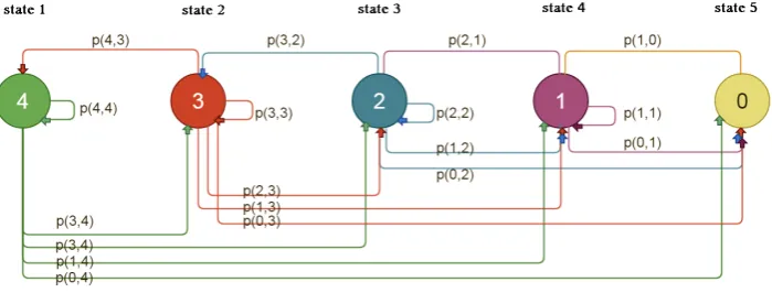
Figure 6.1: Markov chain - example 5 states

Transition rules:

ˆ Markov chain always starts in the state where there are k initial number of suborders left to be stacked

ˆ the next possible moves from state i (except state with 0 suborders) are allowed when:

– there was no suborders stacked→ returns to the same i state

– there has been staked at least one suborder→ going to a state with less suborders (<i)

– the minimum progress limit of the iteration has not been reached (the fill rate is lowered) and there might be a possibility that the blue component splits again the order, but this time, it needs one extra carrier→ goes to state i+1

Computation of transition probabilities and costs

Settings: first of all, data is divided by customers’ orders and then by initial number of suborders. Where there was no training data available (e.g. there were no orders with 5 initial suborders), we used data from the nearest neighbour (with 4 or 6 suborders); in case we could not find any data in the nearest neighbour, we continue and use data from 3 or 7 suborders and so on. In the end, we adapt them such that they could be used for 5 suborders.

For each customer and for each number of initial suborders we computed transition prob-abilities and duration of executing iterations. Transition probprob-abilities are extracted from data by looking at all iterations from the orders, and count how many times LFL went from state i to state j. Thus, the transition probability matrix P ={pij} withpij is the probability that

state i is followed by state j:

E[pij] =

nij

ni

(6.1)

where:

ˆ ni is the number of times state i appeared in the chain

ˆ nij the number of times state i was followed by state j

The time matrix (costs) T = {tij} where tij represents the average time spent from state i to

state j:

E[tij] =

cij

nij

(6.2)

where,cij is the summation of the durations from state i to state j. For each customer and each

Calculation of expected lead time

Define Ti as the time it takes to stack i suborders and it is written as:

Ti = n

X

j=0

(Tj+tij)1(i→j) (6.3)

Where T0 = 0 and 1(i→j) indicates that we jump from state i to state j, so P(i → j) = pij.

Expected lead time is computed after the formula: E[Ti] = pi0ti0 +Pnj>0pij(E[Tj] +tij) for

n >1. Where:

ˆ n– maximal number of suborders to be stacked ˆ pij - probability of going from itoj

ˆ tij - time needed to go fromitoj (so the duration of stackingi−j suborders)

ˆ E[Tj] - expected time to stack allj suborders

The vector notation is:

ET = [I−P]−1ETR (6.4)

ET =     

E[T1] E[T2]

... E[Tn]



   

, P = 

   

p11 p12 .. p1n

p21 p22 .. p2n

...

pn1 pn2 .. pnn



   

and ETR=

n X j=1     

p1jt1j

p2jt2j

... pnjtnj

     (6.5)

withI - identity matrix.

Interval estimation for expected lead time

Prediction interval can be computed for expected lead time of order, depending on initial number of suborders. Assuming that the variable E[Ti] ∼ N(µ, σ2), we computed a 95% confidence

interval for variable Ti solving:

P(−1.96< Ti−E[Ti]

σ <1.96)∼95% (6.6)

with σ2 = Var[Ti] = E[(Ti)2]−(E[Ti])2, E[Ti] and E[Ti] as known from eq. (6.4). The second

moments satisfy

E[T_i2] =pi0E[t2i0] +

n

X

j=0

pij(E[Tj +tij])2 (6.7)

so

ET2= [I−P]−1ETS (6.8)

where

ET2 = 

   

E[T₁2] E[T₂2]

... E[T_n2]



   

and ETS=

n X j=1     

p1j(2E[Tj]E[t1j] +E[t21j])

p2j(2E[Tj]E[t2j] +E[t22j])

...

pnj(2E[Tj]E[tnj] +E[t2nj])

3

First results

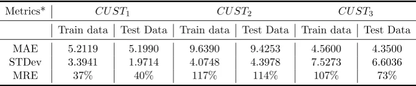
Transition probabilities (P) and durations of iterations (T) were computed on 70% of the each data set (training data), and the expected lead time was computed using the formula presented before. For the testing set, it is known how many initial suborders an orders has (feature 56), and then, we use the related P and T matrices (calculated in the training phase).

Metrics* CU ST1 CU ST2 CU ST3

Train data Test Data Train data Test Data Train data Test Data

MAE 5.2119 5.1990 9.6390 9.4253 4.5600 4.3500 STDev 3.3941 1.9714 4.0748 4.3978 7.5273 6.6036

MRE 37% 40% 117% 114% 107% 73%

Table 6.1: Prediction performance -Markov Chain

Markov chains seem to have a good performance forCU ST1: mean absolute value of5units, small standard deviation of absolute errors ( 3 and 2 for training and testing data respectively), but the mean relative error is large (around 40%), which means that the model tends to over predict. For the other 2 customers, the model does not give good predictions, even if MAE is not that large (10 and 4 units), the MRE is set around 100% for almost every data which means that there are many cases where the error (the difference between the real and predicted lead time) is as large as the real lead time.

4

Confidence Intervals

In general,the accurancy of predictions should improve if we have more data points; in our case, this proved to be true for 2 out of 3 customers. The range of the confidence interval (Appendix E) depends on the number orders used for training the model. For most of theTi variables (Ti

-duration of stacking i suborders e.g. lead time of an order withi initial suborders) the range of the confidence interval is around 1-2 units (Appendix D). On the other hand, in the cases when there were used less than 5 orders for training, the range of the interval increases with 3-10 units. The worst case is for T15 (CU ST3), with only one training order: the range is of 15 units.

The dependence between the size of training data and the range of the confidence interval, for CU ST2 and CU ST3, can be observed in Figure ??.

CONFIDENTIAL

Expected lead time vs mean real lead time

From the difference between the expected lead time and the average real lead times (of the orders with the same initial number of suborders- Appendix D), we can conclude that:

ˆ the same lead time for orders with the same initial number of suborders, it is not ideal. This is how Markov chain model makes the predictions. It predicts the same lead time for orders with the same initial number of suborders. These orders can have different characterics but the model is always indicating the same expected lead time.

ˆ the small difference between the 2 values (expected lead time and mean real lead time) could come from the small size of training data. For CU ST3 we had very small training set (50 orders). Most of leading times with i initial suboers (Ti) were computed based on

computing the real mean lead time, and so the tranzition probabilities and durations were based on similar orders. This could be a reason why the expected lead time is close to the mean of real lead times.

CONFIDENTIAL

5

Improvements

The main idea of improving the lead time using Markov chains, was to improve in some way the transition probabilities and the iterations’ times by including in their construction, informa-tion about the order’s characteristics. Two methods were applied in order to accomplish this: clustering (indirect) and regression(direct).

5.1 Clustering

Improving the lead time prediction using clustering was done by constructing 2 categories of orders and then apply the Markov chain separately on each category. Splitting orders in 2 categories, grouping them by their difficulty and separetly by their lead time, is similar with adding new information about the orders.

There were applied 2 strategies to compute the clusters. Each of this strategies had different variables set for constructing the clusters.

1. Strategy 1 / ”Slow” and ”fast”: is based more on the lead time of the orders. The features included in k-means clustering for all 3 customers were:

ˆ Initial number of suborders (feature 56 - Appendix B) ˆ Predicted lead time from Elastic net regression

2. Strategy 2 / Easy and difficults orders: determined mostly from order’s characteristics. For each customer, different set of features were used. These features (see Table??) were selected based on the results from Elastic net regression: the features with the largest regression coefficient.

CONFIDENTIAL

Clusters were trained with the K-means method (kmeans function from Matlab®Software Statistics Toolbox (Release 2016a; The MathWorks Inc.)). For new orders (testing data), the cluster to which they belong, was determined by looking at the proximity of selected features with the centers of those features, computed by the K-means method.

Strategy 1

The 2 clusters (”slow”,”fast”) are constructed accordingly with their definition (Appendix E): ”slow” cluster is containing orders with large lead time, with more cases, more initial number of suborders etc. and the ’fast’ cluster has the opposite characteristics (small lead time, a few cases, etc.).

The performance of the Markov Chain together with clusterization is in principle decreasing, with one exception. For first and third customer, the mean absolute error and the standard deviation of the absolute errors are increasing while for CU ST2, clusterization has a positive effect.

Metrics* CU ST1 CU ST2 CU ST3

Train data Test Data Train data Test Data Train data Test Data

MAE 5.44 5.99 6.87 7.62 9.08 6.90

STDev 4.54 5.31 6.05 7.78 11.07 7.33

MRE 34% 37% 39% 43% 92% 80%

Table 6.2: Prediction performance -Markov Chain with clustering (strategy 1)

Performance results for the lead time are different for each customer. Comparing these metrics with the ones from simple Markov Chain (Table 6.1), the results for :

ˆ CU ST1 are similar: the mean aboslute error and its standard deviation for the lead time are slightly increasing ( with 0.5-2 units) only MRE (mean relative error) is decreasing with 3%.

ˆ CU ST2 are improving: the mean absolute error is decreasing with around 2 units and MRE with around 60% while standard deviation of absolute errors increases with 2 units.

ˆ CU ST3 are getting worse: MAE,STDev are increasing with 3 units, only MRE is decreas-ing with 10% for traindecreas-ing data.

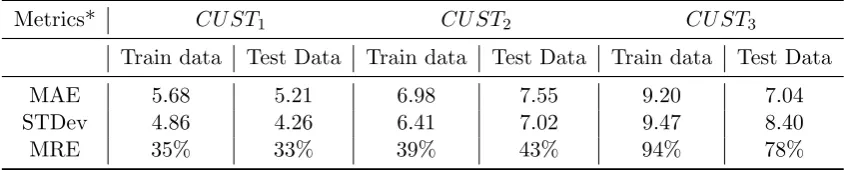
Strategy 2

For strategy 2, the clusters are also constructed correctly: the ’easy’ cluster is characterized bysmalllead time, small value for featuresCONFIDENTIAL. If all these variables (except last one) have high values it means that the orders are more difficult, thus LFL is slower when computing the recipe. If CONFIDENTIAL is smaller it means that the groups contains many products, or that contains products with high volume.

How the orders were split between clusters it can be seen in Appendix E. The performance of the Markov Chain together with clusterization - strategy 2 is similar with the one performed with strategy 1. The differences are very small.

Metrics* CU ST1 CU ST2 CU ST3

Train data Test Data Train data Test Data Train data Test Data

MAE 5.68 5.21 6.98 7.55 9.20 7.04

STDev 4.86 4.26 6.41 7.02 9.47 8.40

MRE 35% 33% 39% 43% 94% 78%

Table 6.3: Prediction performance -Markov Chain with clustering (strategy 2)

5.2 Regression

manner to do this is to approximate the transition probabilities and durations using regression.

Each probability pij will be the dependent variable of the regression. The independent

variables will be the the set of features of the order and the probability computed by the original Markov chain (similar procedure withtij).

While testing this proposal, it has been noted that the probabilities (and durations) that were 0 in the simple MC, now they were estimated to have a small probability. So the situa-tions for which the states had no transition between, pij was 0, now they had assigned a small

probability. Which finally lead to very poor predictions. Thus, the final regression analysis was performed only on pij and tij which had a value different than zero in simple MC.

The regression model used was Elastic net regression. The performance of Elatic net regression, Table 6.4, shows that the estimations ˆtij have,on average, an absolute error of 0.5 units. Still,

MRE suggests that the predicted tij was 1.5 times smaller than the real tij. The situation is

similar for pij. As these results are bad, a poor performance of the Markov chain is expected.

Metrics tij pij

Train data (min) Test Data (min) Train data (prob) Test Data (prob)

MAE 0.6158 0.5773 0.1848 0.1419

STDev 0.6899 0.6533 0.2602 0.2514

MRE 153% 160% 121% 122%

Table 6.4: Prediction performance - Elastic net regression forpij and tij

The under-estimation of tranzition probabilities and durations leads to a big decrease in the predicted lead time: the MRE is negative -70%-80%. We performed the Markov chain model, once with the predicted durations changed, and once with the tranzition probabilities changed ( Table 6.5 -first 2 column, last 2 column respectively).

Metrics Changing Time Changing prob

Train data Test Data Train data Test Data

MAE 11.15 14.25 13.16 15.47

STDev 6.61 7.12 7.72 7.90

MRE -64% -66% -73% -78%

Chapter 7

Sensitivity Analysis

A model can be accepted if it is not sensitive to its specifications or to data. In this chapter we discuss the sensitivity of Elastic net regression and Markov chain. We also discuss the sensitivity of the models when some configuration parameters of LFL are changed.

The idea is to prove that minor changes in data sets, lists of variables, do not alter funda-mentally the results and the conclusions. There are 2 approaches for each model.

For Elastic net, checking if the model is sensitive to the data set is done by dropping 10% of orders, re-estimate the model and check if the coefficients are within ±0.1 of the initial ones. The second test, is to change some specifications of the models and compare the results i.e. the variables set can be changed.

1

Altering data and model’s specifications

Tests were performed only on data ofCU ST1, the one with the largest data set - 560 orders.

Data sensitivity of Elastic net regressionhas been proven by using 90% of the data, and shown that the coefficients of the selected features are within±0.1 compared to the coefficients determined from the entire data set (Appendix F). There were selected new features when perfomed the model on the subset, but their coefficients were very small. There are only 2 features for which the difference of their coefficients are larger than 0.1: CONFIDENTIAL, with 0.11, which has not been selected at all by the original Elastic net run; while the coefficient of feature CONFIDENTIAL has increased with 1.14. These changes explain that, in the 90% subset are included orders which have more ’bad’ cases, thus these changes do not have any negative effect. The performance is slighlty changed, the difference of the mean absolute error between the models is of 0.01 units for training set and 0.02 units for testing set. Thus, Elastic net is not sensitive to data set size.

Metrics* Subset - 90% of original set

Train data Test Data

MAE 2.7222 2.5906

STDev 2.6876 2.0343

MRE 7% 15%

Table 7.1: Prediction performance - Elastic net Regression - 90% subset

mean relative error increased with 1% for training data and 2% for testing data. This shows that the model is sensitive to the data set.

Another test was comparing results of the model when using the estimated transition prob-abilities and the real probprob-abilities (computed based on information of each order). As a result, using the probabilities and durations computed from data of each order has a positive effect on the lead time, in the sense that the performance is better: mean absolute error decreses with 2.5 units and, most importantly, the mean relative error reduces to 6% for training data and with similar results for testing data. This also means that the performance of the model cannot be improved more than that, only by improving the transition probabilities and durations.

Metrics* Train data Test data

Estimated Real Estimated Real

MAE 5.2119 2.6604 5.1990 2.4857 STDev 3.3951 3.0966 1.9714 2.0285

MRE 37% 6% 40% 5%

Table 7.2: Prediction performance - Markov chain - altering probabilities and durations

2

Configuration parameters

LFL is a complex program, it has configuration parameters which, can be different from cus-tomer to cuscus-tomer, but especially from a release to another. Because of continuous improve-ments of the software, some of these parameters are changing and the sensitivity of the models has to be tested again. There were considered the following configuration parameters for the analysis:

CONFIDENTIAL

The 2 models were tested by changing the value (the default value; a smaller and a bigger value than the default one) of 4 configuration parameters: CONFIDENTIAL.

CONFIDENTIAL

Ideally, the models should have similar performances for different versions of the software or different values for the configuration parameters. The resuls of the models are being compared based on the change of the mean relative error (MRE) = M RE−parameterx

M RE−def aulf values. So these values

should be around 1 in order to conclude that the models are not sensitive to changing the configuration parameters.

Elastic Net Regression

In the table ?? the effect of different values for the parameters on the mean relative error (MRE), can be seen. The followings can be concluded:

ˆ by lowering theCONFIDENTIAL, the mean relative error increases a lot; When there is no progress during LFL’s iterations - decreasing the fill rates with a small percentage leads to an increase in the lead time. This change is not captured by any of the features and so MRE increases.

explained. But the difference between the results for the 2 customers come from the fact that for CU ST1, there is also an increase in the number of suborders while for CU ST2, even if the lead time is increasing, this change is not captured by any feature.

ˆ for the parameterCONFIDENTIALthe results are different between the customers. Lowering this parameter leads to a big decrease in the lead time ( mean lead time decreased with almost 30 units). Part of this decrease was also captured by the model (the estimated lead time dropped with 23 units) but no other features had changed (it was expected that the number of initial suborders to change) and so the difference of MRE is caused again by the fact that changing this parameter does not effect any feature. Increasing the parameter means that the fill rates are adjusted more often, which leads to an increase of the lead time (but also an increase of the estimated lead time), thus MRE did not change a lot. The model has captured these changes - connecting the lead time to a slightly different set of features.

ˆ theCONFIDENTIALcould not influence any of the features, and so the model could not connect logically this change in any of the features. The lead time is increasing (with aroundCONFIDENTIAL(mean lead time)) when the timeout for the red component is decreased, and when it is increased, the lead time does not change a lot, but the estimated lead time is decreasing with around CONFIDENTIAL units (the mean predicted lead time)

CONFIDENTIAL

Markov Chains

First of all, the prediction results using Markov Chains are quite bad (mean absolute error are around 20 units) but the cause could be the small data sets (36 and 45 orders). The probabilities and durations of iterations are computed based on very few orders (because for each senario (of having k initial suborders) there are used only the orders which had k initial number of suborders), the model is using for training one, 2 or 3 orders, and based on them the prediction is made.

Nevertheless, Markov Chain model seems not to be sensitive to configuration parameters because most values from table ?? are around 1, thus there are no significant changes in the performance of the model.

Chapter 8

Conclusions and recommendations

Elastic net regressionis a neat solution to estimate the lead time of an order. It is expected that the mean absolute error of the predictions to be around 2-3 units. Nevertheless, the model is sensitive to changes in the configuration parameters. Changing the configuration parameters (which do not have any influence on any features), can significantely affect the per-formance.

Recommendations for Elastic net reggression:

ˆ for training the model, there should be used at least 700 orders

ˆ Elastic net should be trained for each customer separately (better predictions)

ˆ if there are big changes in the configuration parameters (and these changes are not cap-tured by any feature) it might be a solution to create a new feature (which can capture the changes of the configuration parameters) or retrain the model on different data

Markov Chain model tends to overestimate (large MRE); the mean absolute error of estimations is around 7 units. Nevertheless, the model in sensitive to changes in data set size. It has been shown (Chapter 7, section 2) that having 25% less data increases MAE with 0.5 units; however, it is still over-predicting. By analogy, we can expect that more data will decrease the error.

Recommendations for Markov chain model:

ˆ to increase the data set to at least 1000 orders (the mean absolute error expected decrease to 2 units)

ˆ to train it for each customer separately (better predictions)

ˆ for each case with k initial number of suborders, there should be at least 10-15 orders for training

The advantage of this paper: being able to estimate the lead time will allow Vanderlande to schedule orders over their hardware components. They could also estimate further the num-ber of necessary components.

Future work could concentrate on:

1. re-estimating the lead times on data sets of 1000 orders. Check if the performance of the models is increasing

3. try to predict the lead time using a non-linear model

Chapter 9

Glosarry

ACP - Automated Case Picking: concept for fully automated picking of cases for mixed customer pallets or trolleys: the cases are automatically loaded on trays, stored in tray racking and picked by a Case Picker in a sequence determined by a calculated loading pattern

LFL- Load Forming Logic: software module developed by Vanderlande to optimise the loading pattern of shipping pallets or trolleys; capable of calculating and optimising mixed-cases loads

order- a request of new products for one shop. An order consists of a list of orderlines orderline- one row in an order, consisting pf the product, the quantity and the allowed carriers

recipe - a LFL recipe is the output of the LFL module. It contains the stacking information for an LFL order per load carrier

suborder- a part of an order which can fit in a carrier

stack- the result of allocating all products from a suborder to specific locations on a carrier case- a packing unit of a product

Bibliography

[1] Ezekiel M. The Assumptions Implied in the Multiple Regression Equation. Journal of the American Statistical Association . volume 20, Issue 151, pages 405–408. Taylor & Francis, 1925.

[2] Kennard R.W. Hoerl E. Ridge Regression: Applications to Nonorthogonal

Prob-lems. Technometrics. volume 12, Issue 1, pages 69–82. Taylor & Francis, 1970.

[3] Trenkler G. Liski E.P, Toutenburg H. Minimum mean square error estimation in

linear regression. Journal of Statistical Planning and Inference . volume 37, Issue 2, pages 203–214. Elsevier, 1993.

[4] Hemmerle W.J. An explicit solution for generalized ridge regression. Technometrics. volume 17, Issue 3, pages 309–314. Taylor & Francis, 1975.

[5] Tibshirani R. Regression Shrinkage and Selection via the Lasso. Journal of the

Royal Statistical Society. volume 58, Issue 1, pages 267–288. Wiley, 1996.

[6] Tibshirani R. Random Lasso. The Annals of Applied Statistics. volume 55, Issue 1, pages 468–485. Institute of Mathematical Statistics, 2011.

[7] Hastie T. Zou H. Regularization and variable selection via the elastic net. Journal of the Royal Statistical Society. volume 67, Issue 2, pages 301–320. Wiley, 2005.

[8] Akdemir D. Ensemble Models with Trees and Rules. Department of Plant Breeding & Genetics, Cornell University NY, 2012.

[9] Breiman L. Bagging predictors. Machine learning. volume 24, Issue 2, page 123–140. 1996.

[10] Schapire R.E Freund Y. A Decision-Theoretic Generalization of On-Line Learning and an Application to Boosting . Journal of Computer and System Science. volume 55, Issue 1, pages 119–139. Elsevier, 1997.

[11] Schapire R.E. The Boosting Approach to Machine Learning: An Overview. In

Nonlinear Estimation and Classification, pages 149–171. Springer New York, 2003.

[12] B¨uhlmann P. Bagging, Boosting and Ensemble Methods. In Handbook of

[13] Putermann M. Markov Decision Processes: Discrete Stochastic Dynamic Program-ming. John Wiley & Sons, 2005.

[14] Tweedie R.L. Meyn S. Markov Chains and Stochastic Stability. Cambridge Uni-versity Press, 2009.

[15] MacQueen J.B. Some Methods for classification and Analysis of Multivariate Ob-servations. Proceedings of 5th Berkeley Symposium on Mathematical Statistics and Probability. pages 281–297. University of California Press, 1967.

[16] Ng A.Y. Coates A. Learning Feature Representations with K-means. Neural Net-works: Tricks of the Trade. volume 2, pages 281–297. University of California Press, 2012.

[17] Draxler R.R. Chai T. Root mean square error (RMSE) or mean absolute error (MAE)-Arguments against avoiding RMSE in the literature. Geoscientific Model Development. volume 7, page 1247–1250. Copernicus Publications, 2014.

[18] Yovits M. Advances in Computers. Academic Press INC, 1985.

[19] Biswas S. Hripcsak G. Markatou M., Tian H. Analysis of Variance of

Appendix A

Features set

Appendix A is mentioned in Chapter 4. It summarizes the entire set of 56 features with their description and, when is the case, also the formula.

Appendix B

Regression assumptions

Appendix B is mentioned in Chapter 5, section 1.1. It is focused on the assumptions required for applying regression models. Residuals vs fitted,Q-Q plots and Durbin-Watson test which investigate linearity, normality and homoscedascity assumptions respectively.

D-W test CU ST1 CU ST2 CU ST3

p-value 0.0001 0.9774 0.4824 d 1.9459 2.1153 1.8414

Appendix C

Influential features

Appendix C is mentioned in Chapter 5, section 3, the results of Elastic Net regression are discussed . With this method, there were selected 13, 11 and 7 influential features for CU ST1, CU ST2 and CU ST3 respectively. In the following tables there are presented the influential features with their description and with the estimated coefficients.

Appendix D

Confidence Intervals

Appendix D is mentioned in Chapter 5 (section 3) and Chapter 6 (section 4) where the confi-dence intervals for Elastic Net and Markov chains respectively are discussed.

Model: elastic net regression -

CU ST

coeffi-cients

Features Optimal Coefficient Lower bound Upper bound confidence interval confidence interval

8 0.1883 0.1277 0.2489

9 -0.0964 -0.1569 -0.0358

12 0.1692 0.1086 0.2298

13 0.0205 -0.0401 0.0811

20 0.0217 -0.0389 0.0823

27 -0.0439 -0.1045 0.0166

38 0.1051 0.0445 0.1657

39 -0.1459 -0.2065 -0.0853

49 -0.2779 -0.3385 -0.2173

50 0.1148 0.0543 0.1754

51 0.0844 0.0238 0.1450

52 -0.0609 -0.1214 -0.0003

55 0.1836 0.1231 0.2442

Table D.1: CU ST1

Results using as coeffiecients the lower and upper bounds of the confidence interval

Metrics Lower bound (coefficients) Optimal value (coefficients) Upper bound (coefficients) Train data Test data Train data Test data Train data Test data

MAE 4.5725 3.9982 2.8059 2.5056 2.6237 2.3694

STDev 4.0926 2.9111 2.9434 2.1793 2.3883 2.3046

MRE 24% 14% 11% 3% -3% -9%

Model: elastic net regression -

CU ST

Confidence interval for coefficients Results using as coeffiecients the lower and

Features Optimal Coefficient Lower bound Upper bound confidence interval confidence interval

1 0.1113 0.0591 0.1636

2 0.0746 0.0224 0.1269

7 0.0689 0.0166 0.1211

8 0.1198 0.0676 0.1721

11 0.1069 0.0546 0.1591

12 0.1749 0.1226 0.2271

20 0.0041 -0.0482 0.0563

37 0.0194 -0.0329 0.0716

38 0.1023 0.0501 0.1546

40 0.0000 0.0000 0.0000

41 0.1081 0.0558 0.1603

43 0.0390 -0.0132 0.0912

Table D.3: CU ST2

upper bounds of the confidence interval

Model: elastic net regression

-Metrics Lower bound (coefficients) Optimal value (coefficients) Upper bound (coefficients) Train data Test data Train data Test data Train data Test data

MAE 4.3190 4.2385 1.6059 1.2578 2.4652 3.0137

STDev 3.5049 3.3587 1.4417 1.1241 2.6985 3.3582

MRE 53% 91% 3% 2% -46% -87%

Table D.4: CU ST2

CU ST

Confidence interval for coefficients

Features Optimal Coefficient Lower bound Upper bound confidence interval confidence interval

1 0.3752 0.2556 0.4947

4 0.0650 -0.0545 0.1846

8 0.3708 0.2513 0.4903

29 -0.0875 -0.2070 0.0320

30 -0.0235 -0.1431 0.0960

35 0.0596 -0.0600 0.1791

47 0.0277 -0.0918 0.1473

Results using as coeffiecients the lower and upper bounds of the confidence interval

Metrics Lower bound (coefficients) Optimal value (coefficients) Upper bound (coefficients) Train data Test data Train data Test data Train data Test data

MAE 6.9076 5.6634 1.7125 1.1721 3.9786 3.7517

STDev 5.2584 3.2138 1.3072 0.8426 3.4461 2.2361

MRE -6% -3% 42% -1% 89% 1%

Table D.6: CU ST3

Model: markov chain -

CU ST

CONFIDENTIAL

Model: markov chain -

CU ST

CONFIDENTIAL

Model: markov chain -

CU ST

Appendix E

Clustering Analysis

Appendix E is mentioned in Chapter 6 (section 5.1) where are discussed

the improvements for Markov chains by clustering (2 strategies) the orders.

Appendix F

Sensitivity Analysis

Appendix F is mentioned in Chapter 7 where sensitivity analysis for Elastic

Net regression is discussed.

Full data set 90% data set Difference

Feature index Coefficient Feature index Coefficient (absolute)

2 0.0000 2 0.0000 0.0000

9 0.1154 9 0.0338 0.0817

10 -0.0728 10 -0.0534 0.0194

13 0.0847 13 0.0834 0.0014

16 0.0390 16 0.0286 0.0104

19 0.0739 19 0.2190 0.1451

21 0.0000 0 0.0000 0.0000

0 0.0000 20 -0.0458 0.0458

0 0.0000 24 -0.0724 0.0724

0 0.0000 27 -0.1072 0.1072

29 -0.0626 29 -0.0449 0.0177

0 0.0000 31 0.0000 0.0000

39 0.1813 39 0.1893 0.0080

46 0.1101 46 0.1104 0.0003

50 -0.2944 50 -0.2884 0.0061

51 0.1450 51 0.1726 0.0276

52 0.0402 52 0.0178 0.0223

53 -0.1023 53 -0.0626 0.0398

0 0.0000 55 0.0021 0.0021

56 0.1479 56 0.1111 0.0368