Automated ultrasound studies of magnetoelastic effects in rare earth metals and alloys

warwick.ac.uk/lib-publications

A Thesis Submitted for the Degree of PhD at the University of Warwick

Permanent WRAP URL:

http://wrap.warwick.ac.uk/91220

Copyright and reuse:

This thesis is made available online and is protected by original copyright. Please scroll down to view the document itself.

Please refer to the repository record for this item for information to help you to cite it. Our policy information is available from the repository home page.

Automated Ultrasound Studies Of

Magnetoelastic Effects In Rare Earth

Metals and Alloys

Chee Ming Lim

Submitted for the degree of Doctor of Philosophy at the University of Warwick.

Table Of Contents

List of Figures

Acknowledgements

Declaration

Abstract

Chapter 1 Preview

References

Page No.

1 6

Chapter 2 Ultrasonic Techniques And The Magnetic Properties

Of

2.0 Introduction

2.1 Ultrasound Characterisation Of Solids

2.2 Ultrasound Measurement Techniques

2.2.1 Pulse Echo Overlap Technique

2.2.2 Sing Around Technique

2.2.3 Automated Ultrasound Measurement System

2.3 Physical Properties Of Rare Earth Elements

References

Chapter 3 Ultrasound Measurement System And Experimental Method

3.2 Tone-Burst Generator (Matec TB-lOOO)

3.3 Digitiser (SR-9010)

3.4 Amplifiers

3.5 The Control And Processing Software

3.5.1 Temperature Control File

i

3.5.2 Magnet Control File

3.5.3 Waveform Storage

3.5.4 RF Filtering

3.5.5 Temperature Sensor (S2)

3.6 Electromagnetic Acoustic Transducers (EMAT)

3.7 Sample Preparations

References

Chapter 4 Ultrasound Measurements Of Single Crystal Erbium 4.0 Introduction

4.1 The Single Crystal Erbium Sample

4.2 EMAT Acoustic Coupling Efficiency < '

4.3 Velocity Measurements Using EMATs

4.4 Discussion and Conclusion

References

5.2 Ultrasound Measurements OfTm Using Quartz Transducers 65

5.3 Ultrasound Measurements OfTm Using In-plane Radially

Polarised EMAT 71

5.4 Contour Plot of EM AT Signal Amplitude for Tm 72

5.5 Conclusion . 74

References 75

Chapter 6 Ultrasound Measurements Of Erbium-Thulium Alloys

6.0 Introduction 77

6.1 The Er-Tm Samples 77

6.2 Elastic Constants Measurements 78

6.2.1 c-axis Measurements 79

6.2.2 a-axis Measurements 82

6.3 Ultrasound Studies Of Er-Tm Using EMATs 84

6.3.1 EMAT Generated Shear Wave Velocity

Measurements 84

6.3.2 EMAT Generated Longitudinal Wave

Velocity Measurements 86

6.3.3 EMAT Signal Amplitude Measurements 86

6.4 Contour Plot of EMA T Signal Amplitude for Er91.6% Tms.4% 89

Chapter 7 Conclusion And Further Work

References

Bibliography

93

List Of Figures

Chapter 1

Figure 2.1. Wave propagation along the non-symmetry direction in an anisotropic

media.

Figure 2.2. Slowness surfaces for Er at 300 K.

Fgiure 2.3. Pulse echo overlap system~

Figure 2.4. Schematic of Magnetic ordering in Er.

Figure 2.5. Schematic of Magnetic ordering in Tm.

Chapter 3

Figure 3.1. Schematic of experimental setup.

Figure 3.2. Schematic of cryostat and superconducting magnet.

Figure 3.3. Software flow chart for a typical ultrasound velocity measurement.

Figure 3.4 (a) Reference pulse, (b) Second pulse and (c) Demodulated output

waveform.

Figure 3.5. Sample holder.

Figure 3.6. Spiral pan.:.cake coil EMAT producing in-plane radially polarised shear

Chapter 4

Figure 4.1. H - T phase diagram for single crystal Er.

Figure 4.2. ac susceptibility measurements for Er.

Figure 4.3. EMAT acoustic coupling efficiency as a function of temperature for Er

with applied magnetic field at 0.5, 1.0 and 2.0 T.

Figure 4.4. Square root of EMAT signal amplitude versus c-axis applied magnetic

field. Er sample.

Figure 4.5. C44 versus temperature for Er with c-axis applied field at 1 T.

Chapter 5

Figure 5.1. A tentative magnetic phase diagram ofTm.

Figure 5.2. Magnetic moment measurements ofTm at 5 K.

Figure 5.3. ac susceptibility versus temperature for Tm with 0.1

De

Figure 5.4. Slowness surfaces for Tm at 300 K with CJ3

=

Figure 5.5. C33 as a function of temperature for Tm at zero field.

Figure 5.6. C33 as a function of temperature with applied magnetic field along the c-axis.

Figure 5.8. Signal processed C₃₃ (zero field) data and a 3 point nearest neighbour averaging applied.

Figure 5.9. Longitudinal wave attenuation as a function of temperature for Tm. Wave

propagating down the c-axis at zero applied field.

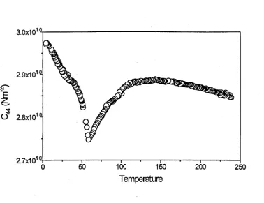
Figure 5.10. C44 as a function of temperature at zero applied field.

Figure 5.11. Signal processed zero field C44 data as a function of temperature with 3 points averaging applied.

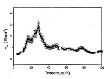
Figure 5.12. Zero field shear wave attenuation (0.44) versus temperature. Wave propagating direction down the c-axis.

Figure 5.13. C44 as a function of temperature for Tm with c-axis applied field at 0.5, 2.0 and 3.0 T.

Figure 5.14. Shear wave attenuation as a function oftemperature for Tm with c-axis

applied field at 3 T. Shear wave propagated down c-axis.

Figure 5.15. C66 as a function of temperature for Tm.

Figure 5.16. CII as a function of temperature for Tm.

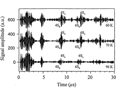
Figure 5.17. Waveforms of EM AT generated in-plane radially polarised shear wave ..

propagating down the c-axis of Tm with sample temperature at 60, 70 and 96 K.

C-axis applied magnetic field at 2 T.

Figure 5.18.- EMA T ~easured C44 as a function of temperature for Tm with c-axis applied field at 0.6 and 1.5 T.

Figure 5.20. Ho - T plot of EM AT signal amplitude for Tm. Ho and shear wave propagation along the c-axis of the single crystal Tm.

Chapter 6

Figure 6.1. C44 versus temperature for Er91.6%Tms.4% at zero field.

Figure 6.2. Shear wave attenuation versus temperature at zero field for Er91.6%Tms.4%.

Figure 6.3. C44 versus temperature for Er91.6%Tms.4% with c-axis applied field at 0.5, 0.75, 1.0 T.

Figure 6.4. C44 versus temperature for Er91.6% Tms.4% with c-axis applied field at 0, 3 and 4 T.

Figure 6.5. Shear wave attenuation as a function of temperature for Er91.6%Tms.4% with c-axis applied field at 3 T.

Figure 6.6a. C33 as a function of temperature for Er91.6%Tms.4% at zero field.

Figure 6.6b-d. Expanded graph of figure 6.6a.

Figure 6.7. C33 as a function of temperature for Er91.6%Tms.4% with c-axis applied field at 0.5 T.

Figure 6.8. C33 as a function of temperature for Er93.3%Tm6.7% with c-axis applied field at 0, 1, 2; 3 and 4 T.

Figure 6.10. CII as a function of temperature for Er91.6%Tms.4% with a-axis applied magnetic field at 0, 0.5 and 1 T.

Figure 6.11. Longitudinal wave attenuation as function of temperature at zero field. Wave propagation down the a-axis.

Figure 6.12. C66 as a function of temperature for Er91.6% TmS.4% with a-axis applied field at 0, 0.5, 1 and 2 T.

Figure 6.13. B-axis polarised shear wave attenuation as a function of temperature for Er91.6%Tms.4% at zero field. Wave propagated down the a-axis.

Figure 6.14. EMAT measured C44 as a function of temperature for Er91.6%Tms.4% with c-axis applied field at 0.5,0.75 and 1 T.

Figure 6.15. EMAT measured C33 as a function of temperature for Er91.6%Tms.4% with c-axis applied field at 0.5, 0.75 and 1 T.

Figure 6.16. EMA T signal amplitude versus temperature for Er91.6% TmS.4% with c-axis applied field at 0.5, 0.75 and 1 T.

Figure 6.17. Waveforms of EMA T generated in-plane radially polarised shear waves propagating down the c-axis of Er91.6%Tms.4% at 77 K.

Figure 6.18. Longitudinal EMAT signal amplitude as a function of temperature for Er91.6%Tms.4% with c-axis applied field at 0.5,0.75 and 1 T.

Declaration

The work contained in this thesis is my own except where specifically stated

otherwise, and was based in the Department of Physics, University of Warwick from

January 1995 to April 1998. No part of this work has been previously submitted to

this or any other academic institution for admission to a higher degree. Some of the

Abstract

Ultrasound studies of single crystals of Er, Tm and alloys of Er-Tm were carried out as a function of temperature (4.2 - 300 K) and applied magnetic field (0 - 5 T). The elastic constants of these materials were measured and anomalies in the elastic constants were observed. The ultrasound data were compared with reported results from other material characterisation techniques and the magnetic phases and transition temperatures of the materials were then identified. The effects of the application of magnetic field on the magnetic ordering of the materials were studied using the ultrasound method. In Er-Tm there was evidence of applied field (a-axis field and c-axis field) induced ordering in the cycloid phase and c-c-axis applied magnetic field of > 3 T resulted in the ferrimagnetic to ferromagnetic transition in Tm.

A commercial ultrasound measurement system was modified and adapted for use in this work. The modified system enables the ultrasonic velocity and attenuation to be measured as a function of: (a) temperature, (b) applied magnetic field and (c) frequency. The present system was enhanced to work with less efficient ultrasonic transducers such as quartz and electromagnetic acoustic (EMAT) transducers.

This work looked at the design and feasibility of using EMA Ts to generate ultrasound in single crystals of the rare earth metals and alloys. EMATs generating (a) in-plane radially polarised shear waves and (b) longitudinal waves were made and shown to work on these materials. The use of EMA Ts meant that ultrasound

measurements could be conducted in the non-contact regime, i.e. no acoustic couplant is required between the sample and transducer. EMATs are particularly useful in this work where the sample and transducer are subjected to repeated temperature cycles over a wide temperature range (4.2 to 300 K) and acoustic couplant can fracture.

Chapter 1

Preview

A wave is characterised by its amplitude, direction of propagation, polarisation,

frequency and wavelength. The characteristics of an ultrasonic wave can change as it

interacts with the medium through which it propagates. The ultrasonic wave interactions

can be observed via the changes in the wave polarisation, velocity and attenuation.

Several of the recognised wave interaction mechanisms are listed and discussed in

Truell et al. (1969). Measurement and monitoring of the ultrasonic wave velocity (group

velocity) and attenuation is the basis of ultrasound measurement.

The aims of this work are:

(a) to adapt a commercial ultrasound measurement system (Matec DSP·8000) for use in

the ultrasound study of single crystal rare earth metals and alloys.

(b) to perform ultrasound measurements on single crystals of erbium (Er) thulium (Tm)

and the binary alloy Er· Tm as a function of temperature and applied magnetic field.

In this work the elastic properties of single crystal rare earth metal; Er, Tm and

their binary alloy (Er-Tm) are studied using ultrasound measurement techniques. The

ultrasonic wave velocities are measured as a function of temperature and applied

magnetic field. The relationship between the ultrasonic velocities and the elastic

constants (moduli) for these samples (hexagonal close-packed structure) are described in

chapter 2. While the theoretical aspects of ultrasonic wave propagation in hexagonal

close-packed crystal are being described, the experimental considerations are also

discussed. This is then followed by a brief description of the different ultrasound

measurement techniques used in the study of single crystal rare earth metals.

Section 2.3 serves as a generic section introducing the general properties, with

emphasis on the magnetic structures, of Er and Tm. The magnetic structures of these

metals have been extensively studied, namely by x-ray and neutron diffraction

techniques [Cable et al., 1965], [Habenschuss et al., 1974], [Cowley and Jensen, 1992],

[Astrom et al., 1991], [Koehler et al. , 1962] [McEwen et al. , 1995]. Several magnetic

phases have been identified in these metals.

Although the magnetic properties of these samples have been studied using other

material characterisation techniques, the results from the ultrasound measurement

shown in this thesis are believed to be the first reported for the single crystal ofTm and

Er-Tm. Furthermore: this work is believed to be the fIrst reported ultrasound studies of

single crystal Er, Tm and Er-Tm using a miniature EMAT. The use of an EMA T enables

the ultrasound measurements to be perfonned in the

non-conta~t

the sample and transducers are often subjected to the extreme of temperatures (4.2 K to

300 K). If a contact ultrasound measurement method is used, the choice of acoustic

couplant becomes critical. The wide temperature range and repeated temperature cycling

causes severe thermal stress on the acoustic couplant which often results in the breaking

of the acoustic couplant, i.e. the sample becomes acoustically detached from the

transducer. This can be particular problem for some of the rare earth materials which

can expand along the c-axis while contracting along the basal plane. The EMA T

acoustic coupling efficiency, however, is dependent on the magnetic and electrical

properties of the sample. One would expect a great variation in the EMA T acoustic

coupling efficiency from sample to sample. Furthermore, these properties which the

EMAT acoustic generation efficiency is dependent on are not single valued but are

dependent on the temperature, pressure and applied magnetic field. For magnetically

anisotropic materials, the direction of the applied magnetic field also affects the EMAT

acoustic generation efficiency.

Chapter 3 describes the ultrasound measurement system. The ultrasound

measurement system used in this work is a modified version of a Matec DSP-8000. The

aim is to produce an automated ultrasound measurement system which can perform

velocity and attenuation measurements as a function of temperature, frequency and

applied magnetic field. In chapter 3 the process of integrating the DSP-8000 with an

Oxford Instruments cryogenic system and super-conducting magnet is described. At the

initial stage of this work a large proportion of time was spent in modifying the original

DSP-8000 software. Modifications to the software were

necess~

software are described in section 3.5. Chapter 3 also describes the hardware

modifications to enable the use of EMAT and quartz transducers. Most commercial

ultrasound measurement systems are designed to drive lead zirconate titanate (PZT) or

similar transducers. The acoustic generation efficiency of PZT transducers are orders of

magnitude better than those of quartz transducers and EMAT and therefore additional

amplifiers and filter circuit are required to improve the signal to noise ratio. The EMA T

design considerations are discussed in section 3.6. Chapter 3 ends with the description

of sample preparation.

The experimental results for the Er, Tm and Er-Tm samples are shown and

discussed in chapters 4, 5 and 6 respectively. The ultrasound measurements using spiral

coil EMAT, generating in-plane radially polarised shear wave, was tested on the single

crystal Er sample. The aims of this preliminary test is to:

(a) monitor the performance of the in-house design and manufactured EMAT coils.

(b) evaluate the performance of the automated ultrasound measurement system.

(c) study EMAT acoustic coupling efficiency as a function of temperature and applied

magnetic field on single crystal of Er.

The EMAT ultrasound measurement results were then compared with the

ultrasound measurement results reported by Palmer et al. (1974) and Eccleston and

Palmer(1992). The shortfalls of the automated ultrasound measurement system were

noted. The results from the preliminary EMA T ultrasound measurement show

~

spectacular changes in EMA T acoustic coupling efficiency for the different magnetic

magnitude was observed close to the magnetic phase transition temperatures. Hence

demonstrating the possibility of using the EMA T acoustic coupling efficiency to detect

magnetic phase transitions in the rare earth metals.

In chapter 5 the results from the ultrasound measurements of the single crystal

Tm sample are presented. The elastic moduli (Cl h C33, C44 and C66) as a function of

temperature and applied magnetic field were measured. Several anomalies in the elastic

moduli measurements were observed. EMATs were also used in the ultrasound

measurements of the Tm sample. The EMAT signal amplitude was used to construct a

tentative magnetic phase diagram for the Tm sample.

Two binary alloys of Er and Tm were studied. Both samples were in the form of

single crystals. The compositions, as atomic weight percentage, for the alloys are;

Er93.3%Tm6.7% and Er91.6%Tms.4%. The elastic moduli of the samples were measured as a

function of temperature and applied magnetic field. The results from these ultrasound

measurements are presented in chapter 6. Longitudinal EMA T was tested on the

Er91.6%Tms.4% sample. The results show distinct differences in the EMAT acoustic

coupling efficiency between shear wave and longitudinal wave generation. A tentative

magnetic phase diagram of Er91.6%Tms.4% has been constructed using the shear wave

EMAT signal amplitude.

The overall performance of the automatic ultrasound measurement system

system are discussed and suggested as further work. The use of EMAT in ultrasound

studies of rare earth metals is discussed in chapter 7.

References

Atoji M. 1974, Solid State Commun., 14, pp1047.

Astrom H.U., Nogues J., Nicolaides G.K., Rao K.V. and Benediktsson G. 1991 J. Phys.: Condens. Matter 3, pp7395-7402.

Cowley R.A. and Jensen J. 1992, J. Phys. Condens. Matter 4 pp9673-9696.

Eccleston R.S. and S.B. Palmer 1992, J. Magnetism and Magnetic Materials, 104-107, ppI529-1530.

Koehler W.C., Cable J.W., Wollan E.O. and Wilkinson, M.K. 1962, Phys. Rev. B 126,

pp1672.

Palmer S.B., E.W. Lee and M.N. Islam 1974, Proc. Roy. Soc. Ser. A338, pp34 1.

Truell R., Elbaum C. and Chick B.B. 1969, Ultrasonic Methods in Solid State Physics,

Chapter 2

Ultrasonic Techniques And The Magnetic Properties Of Er

And Tm.

2.0 Introduction

The aim of this chapter is firstly in section 2.1 to provide the necessary

background to the ultrasound measurements associated with this work. This is followed

by an introduction to ultrasound measurement techniques, with emphasis on the

pulse-echo method. In the ultrasonic theory section practical considerations are also discussed

and in section 2.3, the magnetic properties of Er and Tm are introduced.

2.1 Ultrasound Characterisation Of Solids

The fundamental aim of ultrasound measurements is to generate, propagate and

detect ultrasonic waves. Changes in the wave characteristics, Le. velocity and

.'

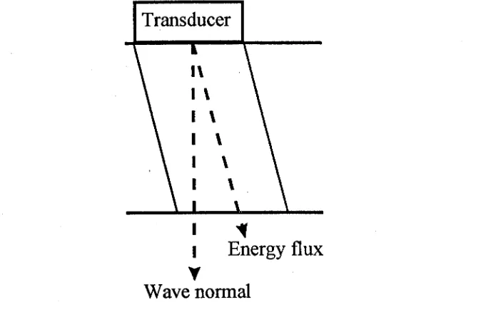
attenuation, then imply physical changes in the sample.

In general, three distinct waves can be propagated along any one direction in a

propagating along a non-symmetry direction in an anisotropic medium, the wave energy

does not coincide with the wave front normal, see figure 2.1, and as a consequence the

ultrasound beam is steered. In ultrasound measurements it is the wave front velocity

(group velocity) that is measured [Musgrave, 1970]. In general, the group velocity and

phase velocity are not equal. In this work the interest is in propagating ultrasonic waves

along the principal axes of the hexagonal close-packed (hcp) structure. The basal plane

is isotropic and all the wave surfaces are circular. This means that the velocity and wave

surfaces coincide. Any section containing the c-axis (orthogonal to the basal plane) has

non-circular slowness surfaces (sm-I) as illustrated in Figure 2.2 for Er. The longitudinal

slowness surface is indicated by L and the shear slowness surface, SI (polarisation along

the b-axis), is shown dotted whereas the other shear slowness surface, S2 (basal plane

polarised), is shown in solid line. If the waves propagate along the c-axis direction the

two shear slowness surfaces coincide, hence there is no ambiguity in the shear velocity

measurement. However, if the wave is propagated off the c-axis, say at 45° to the c-axis,

the SI and S2 surfaces are separated implying that one would obtain two different shear

velocities, as expected.

Simple propagation theory assumes plane waves. However it is difficult if not

impossible to achieve the plane wave condition. The form of the propagation is

determined by the transducer size and resonant frequency. Considering a continuous

--wave transducer modelled as a piston radiator the near field extent is given by; N

=

D2/4A. and the ultrasound beam divergent half angle is given by

e

=

Transducer

...

I

Energy flux

y

Wave normal

Figure 2.1. Wave propagation along the non-symmetry direction in an anisotropic

media. Wave propagation direction and the energy flux direction do not coincide.

90

C-axIS

1801+---~---~----~---H~----~

270

A

- Figure 2.2. Sloweness surfaces oflongitudinal wave, L, and shear waves, SI and 82,

transducers used are 2.0 mm in diameter and resonant at 10 MHz, giving for a typical

longitudinal velocity of 3200 ms·1 , ')..,

=

e

= 11

=

And for a typical shear velocity of 1800 ms·1, ')..,

=

e

=

=

mm.

In the near field the on-axis maxima and minima become less pronounced for a

transducer driven by a tone burst; tone-bursts of less than 5 cycles are used for the present work so it is expected that (with sample thickness of around 4mm) near field

effects should not cause any problems~

We will now develop the relationship between the elastic moduli and ultrasonic

velocity for a hexagonal crystal. It must be emphasised that plane waves are considered

and the medium is assumed to be non-dispersive. The displacement, s, of a particle, in

the medium in which a stress wave propagates, is related to the elastic modulus, C, as

[Truell et al., 1969];

(2.l)

where p is the density of the medium and the displacement; Sx

=

being the amplitude of the displacement at time t = O. The subsript x can be replaced by

ij,k or 1. 0) the wave angular frequency, wavevector k

=

normal to the wave front and the subscripts i,j, k and 1 can take the values 1,2 or 3. For

equation 2.2. in the matrix notation, i.e. ClIlI == _{ClI, C1I22} == _{Cl2, Cl133} == _{Cl3, C3333} ==

ClI Cl2 Cl3

-Cl2 Cl3 C33

-

C44

-C66

=

Using equation 2.1 and equation 2.2 a set of equations are obtained;

[clln~

+

~

(C

C

)n;

+

C44n~

- pv']

s,'

+

[~

(C

+

C

)n,n,

]S"

+

+

=

+

+

Clln~

+

C44n~

2 "

+

+

=

(2.3)

[(C I3

+

+

+

+

[C44 {ni :- nn

+

C33n~

=

(C44 - pV2)SOI = 0

(C44 - pV2)S02

=

(C33 - pV2)S03

=

(2.4)

The solutions to equation 2.4 implies that C44 can be obtained by measuring the shear

wave velocity propagated down the c-axis with polarisation parallel either to the a-axis

or b-axis. The C33 modulus can be obtained from the velocity measurement of the

longitudinal wave propagated down the c-axis. Directing waves down the a-axis, nl

=

I, n2 = n3 = 0 reduces equation 2.3 to,

(CIl -p~ )Sol

=

[(Cll - Ci2)12 - pV2]s02

=

(C44 -p~)s03

=

(2.5)

The solution to equation 2.5 shows the longitudinal velocity measurement would

provide the value for CII and shear wave velocities measurements with polarisation

along the c-axis would give C44 and if the shear wave polarisation is along the b-axis

C66

=

waves along the c-axis and a-axis therefore give only C33, C44, ClI , C I2 and C66. To

determine

C\3,

required. A typical direction in which the wave is propagated and its velocity measured

values into equation 2.3 gives the solution for the transverse wave with polarisation

along the b-axis;

(2.6)

And the combination of the transverse and longitudinal wave solution is;

and hence the determination of CI3.

From the above discussion we see that the elastic moduli for the hcp crystal, i.e.

Cll, C33 , C44, CI2 and C66

=

shear velocities measurements with wave propagated down the principal axes of the

crystal. Due to the size of the samples it was not possible to do a 45° cut between the c

and a axes, thus C I3 was not measured.

Apart from the losses at the transducer-sample boundary, changes in the acoustic

Wave characteristics can be caused by several interaction mechanisms as discussed by

Truell

et aC(1969).

the direct scattering at the boundaries and the magnetoelastic losses due to domain wail

motion, domain rotation and spin-phonon effects. In the review by Bar'yakhtar and

is small it can have significant effects at magnetoacoustic resonance in magnetic

systems having magnetic anisotropy and at magnetic phase transitions. Magnetoacoustic

resonance occurs when the frequencies and wave vectors of magnons and phonons

having the same symmetry coincide. Magnetoacoustic frequencies are typically - 109

Hz, well above the frequencies involved in this work - 107 Hz. The theory on the

magnetoelastic interaction in ferromagnets are discussed by Povey et al. (1980) and

Buchel'nikov and Vasil'ev (1992). The acoustic generation in ferromagnets was shown

to be contributed by two main types of process; at low applied magnetic field the

acoustic generation is dominated by the spin-lattice coupling as a result of domain wall

motion and domain rotation whereas a modified Lorentz mechanism dominates in the

high field regime.

2.2 Ultrasound Measurement Techniques

In this section different ultrasound measurement methods are introduced and

discussed. Ultrasound measurebent systems can either function in the pulse-echo mode

or continuous wave (cw) mode. The discussion in this section concentrates only on

.-ultrasound measurement techniques working in the pulse-echo mode.

In the pulse echo mode, ultrasound is generally produced as burst of pulses,

generally in the form of a tone-burst (packet of acoustic energy). A tone-burst pulse

consist of one or more wave cycles. The width of the tone-burst is determined by the

close to the resonant frequency) of the acoustic transducer. The preferred tone-burst

profile, i.e. the shape enveloping the wave cycles, is a Gaussian wave envelope which

provides a continuous frequency domain.

The detection of the acoustic wave can either be by the same generating

transducer or by a different receiver transducer. In this work the so-called send-receive

mode is used with one transducer both sending and receiving. The through transmission

method is preferred for highly attenuating samples. In most cases amplification of the

received signal is necessary. Several amplifications stages and filters may be used to

improve the signal to noise ratio.

Ultrasound measurement techniques can be designed to; (a) be highly sensitive

to velocity and attenuation changes or (b) measure accurately absolute velocities. In this

work the interest is in the detection of velocity change, I1v/v

=

are described below starting with the pulse echo overlap technique.

2.2.1 Pulse Echo Overlap Technique

The pulse echo overlap technique is a very sensitive and high precision

technique.

Iti

time offlight is defined as the time taken by the ultrasonic pulse to travel from the

acoustic transmitter, through the sample, to the receiver. The sample is prepared with

surfaces and attached to the sample with an acoustic couplant, e.g. ultrasonic gel. The

ultrasonic pulse is transmitted from the transducer through the acoustic couplant and

into the sample. The acoustic couplant allows most of the ultrasound energy to be

transmitted into the sample. The ultrasonic pulse then propagates through the sample

until it reaches a boundary, an acoustically mismatched surface where most of the

ultrasound energy is reflected back into the sample. The ultrasonic wave then propagates

through the sample again before reaching the tranducer via the acoustic couplant. The

total time taken, including electronic delays, is the time of flight of the pulse echoes.

The basic setup of a pulse echo overlap system is shown in figure 2.3 as

described in Hellier et al. (1974). A frequency synthesizer triggers the x-axis of the

oscilloscope and this is frequency divided at a decade fraction. This is then use to trigger

the RP generator which in turn pulse the acoustic transducer.

In

transducers are placed on opposite sides of the samples surface. The received acoustic

signal is then amplified and fed into the y terminal of the oscilloscope. When the

."

repetition rate of the frequency synthesizer, after adjustment, matches the propagation

time of the ultrasound signal through the sample plus electronic delay the ultrasound ""

pulse echoes appear to be overlapped on the display screen of the oscilloscope. The

oscilloscope display is enhanced by feeding part of the output for the frequency divider

into the z mod of the oscilloscope. This increases the brightness over the two

oVerlapping pulse echoes. The time of flight of the pulse echoes is obtained from the

Frequency Synthesizer

x z y

Oscilloscope

Frequency Divider

Double Strobe delay generator

Amplifier

The use of a manual pulse echo overlap ultrasound measurement system in this

work is tedious and labour intensive. For each measurement the operator has to align the

pulse echoes and then take the reading off the frequency meter plus the sample

temperature reading and the applied magnetic field reading. Changes in velocity close to

magnetic phase transitions can occur abruptly. It can become very difficult to keep track

with the velocity changes while having to take all the readings manually. Previous

workers in the group (ultrasound group headed by S.B. Palmer) have introduced a

semi-automatic pulse echo overlap system [Patterson, 1986]. In the semi-semi-automatic pulse

echo overlap system the operator is only required to align the pulse echoes and manually

activating a PC to capture and store the frequency readings and the sample temperature

readings.

2.2.2 Sing Around Technique

In the sing around technique a feedback mechansim is used to measure the time

of flight of the ultrasound pulse echoes. A transducer is used to generate the ultrasound

While another is used as a receiver. An initial rf pulse is used to trigger a pulse generator

to generat~ the ultrasound. The received signal is then amplified and fed back to the

pulse generator to produce another pulse. Ultrasonic pulses are thus generated and

transimitted through the sample continuously. The reciprocal of the repetition rate is the

time taken for the pulse to travel through the sample plus the electronic delays. Absolute

electronic delays. The sensitivity of the system is typically I1v/v::z 10-5 [Jiles, 1979]. The system used by liles (1979) was not automated.

2.2.3 Automated Ultrasound Measurement System

One automated ultrasound measurement system designed and constructed by

former workers of this group not only uses a PC to control the experimental parameters

and to acquire and store data, it also can determine the time of flight of the pulse echoes

[Eccleston, 1991]. Communications between PC and the instruments is via the IEEE

488 interface bus. This system was a leap forward from previous ones.

A transducer is repeatedly pulsed by a Matec tone-burst generator at fixed

frequency, pulse width and output voltage. The ultrasonic waveform was then captured

using a Hewlett-Packard (HP54201A) digital storage oscilloscope. Two successive

pulse echoes are selected, i.e. time base of the digital oscilloscope adjusted to display

..

only two pulse echoes on the display screen. The data capacity per trigger is 1000 data

points. The data are then transferred to the PC. Once in the PC the data are processed to

extract the time of fight of the pulse echoes. To do this the algorithm looks for the zero

crossing (V~O) points of the cycles in each pulse. A quadratic function is then fitted

oVer the data points. The root (real part) of the quadratic function gives the zero

crossing point in the time domain. The time of flight of the pulse echoes are determined

successive pulse echo. The difference in the roots for each pair of cycles, L1t, are then

determined and the average value calculated. The system used by Eccleston (1991) can

also work out the ultrasonic attenuation by measuring the relative change in amplitude

of the two selected pulse echoes.

The inherent problem with the system, or any automated system, is the reliance

on well defined and non-distorted pulse echoes. Error can be easily introduced in the

Velocity and attenuation measurements. For example the method of attenuation

measurement described above assumes that an exponentially decaying function can be

fitted over a series of ultrasonic pulse echoes in the ultrasound waveform. Any mode

converted waves running through the waveform can interfere with the main pulse

echoes and the envelope of the pulse echoes is no longer an exponentially decaying

function. A commonly used method of ultrasonic attenuation measurement is to fit an

exponential function over several pulse echoes in the pulse echo train as they are being

displayed on the oscilloscope. Fitting is carried out by varying the time constant on the

function generator producing the exponential function. The quality of fit is rarely perfect

and is subject to the discretion of the operator.

Similarly the error in the velocity determination Can result from the distortion of

the pulse echoes. In such circumstances the zero points for each cycles can not be

paired up correctly. It must be pointed out that even a manually operated system, such as

the pulse echo overlap system, requires reasonably well defined pulse echoes for the

cycles to be matched (overlapped) accurately. In a manually operated system the

2.3 Physical Properties Of Rare Earth Elements

This is a generic section introducing the rare earth elements of erbium and

thulium. For a detailed description of the physical and chemical properties of the rare

earth the reader can refer to the Handbook on the Physics and Chemistry of Rare Earth

(Gschneidner and Eyring, 1978). A comprehensive description of the electronic

structure of these elements and their alloys are reported by Coqblin (1977). Details of

the magnetic properties of rare earth metals can be found in Elliot (1972).

The rare earth elements, also referred to as the Lanthanide series, starts with

Lanthanum with atomic number 57 and ends with Lutetium having atomic number 71.

The atomic radii, defined as half the distance between nearest neighbours, range from

-1.83

A

A

linear [Hall

et al.,

< 64, have the double hexagonal close-packed (dhcp) structure. The non hcp or dhcp .'

structure elements in the s'eries are Ce, Srn, Eu and Yb. Srn and Eu have rhombohedral

and body-ce~tred cubic resp~ctively. 'Ce has the y face-centred cubic (fcc) at normal

temperature and pressure but can change into the a fcc at low temperature or at high

pressure. Yb has a fcc structure at room temperature and normal pressure. The

in their chemical properties which contributed to much of the difficulties in the

purification process. Some of these elements are not rare at all but due to the difficulties

encountered in the purification process they are labelled rare earth elements. In most

circumstances, the electronic configuration of these elements is; 4f, Sdi, 6s2, where n

can take the number 0 to 14. In general, the 4fwave functions from the nearest

neighbours do not overlap and the 4f orbital is at least 10 times smaller than the atomic

radius. The relatively small 4f shell makes it possible to treat the atoms as isolated

trivalent ions. The distribution of the conduction electrons is as follows; one electron in

the 5d shell and two electrons in the 6s shell. The distribution of the 4f electrons follows

Hund's rule. The magnetic moment is given by; J.l

=

Bohr magneton, g] the Lande factor defined as;

J(J

+

+

+

+

gJ = 1

+

+

and J the total angular momentum with

J

=

=

momentum respectively. Er and Tm, being heavy rare earth metals have their total

angular momentum described by J

=

+

=

=

. == 15/2 and (b) Tm; S

=

=

=

7.6J.lB for Er and Tm respectively, while the measured values are 9.5J.lB and 7.62J.lB

[Coqblin, 1977]. The very good agreement between the theoretical and the experimental

behave like independent trivalent ions is valid (only to the first approximation). The 4f

.•

electrons thus dictate the magnetic properties of the metals.

Er has a metallic grey appearance with density p = 9.145 gcm-3• The lattice

parameters are; a

=

A

A

rare elements have been extensively studied using x-rays and neutron diffraction

methods. The phase diagram of Er has been constructed by several workers with the

early work performed by Cable et al. (1961) on poly-crystalline samples of Er.

Improvements in the metal purification process provided sufficient quantity of starting

material at reasonable cost for the production of single crystals. In the pioneering work

on Er reported by Cable et al. (1965) three distinct magnetic phases were observed

apart from the room temperature paramagnetic phase. The Neel temperature of Er is at

87 K with the magnetic moments aligned along the c-axis and sinusoidally modulated.

Detailed studies conducted by Habenschuss et a/. (1974) and Atoj i et al. (1974) showed the change in the modulation of the moments as a function of temperature.

Initially the anti-ferromagnetic phase exhibits a modulation period of just under 8

atomic layers at 84 K, q=1I4 to just under seven atomic layers at 52 K, q =217. The next distinct phase identified by Cable et a/. (1965) is between 54 K and Tc = 18 K. A basal

plane component is observed which has the same period of modulation as the c-axis

components; High resolution synchrotron x-ray scattering studies reported by Gibbs et al. (1986) provided evidence oflock-in transitions with q = 114, 6/23, 5/19, 4115 and 2/7. Below the Curie point the magnetic moments are aligned with a cone ferromagnetic

structure. Recent work by Cowley and Jensen (1992) provide detailed discussion on the

c-C-axis

+

+

I':

₊

~

~

~

t

~

+

t

~

t

18K

54K

87K

Figure 2.4. Magnetic ordering of Er. Neel temperature occurs.at 87 K with magnetic

axis magnetic phase diagram of Er has been constructed by McMorrow et al. (1992),

showing the complexity of the magnetic structure between 18 K and 52 K. The three

distinct magnetic ordering structures of Er are shown schematically in Figure 2.3.

Other experiments besides the neutron and synchrotron x-ray diffraction studies

have been performed on Er, i.e. ultrasound [Ecc1eston et al., 1992], thermal expansion

and magnetostriction [Zochowski et al., 1995], ac susceptibility and resistivity [Watson

et aI, 1995] and magnetisation [Snigirev et al., 1992]. Note that the ultrasound studies

conducted by Eccleston et al. (1992) used quartz transducers for the acoustic generation whereas in this work the focus is on EMA Ts and can be considered as a further

extension to the studies reported by Eccleston et al. (1992).

Tm has similar physical properties to Er. Its density is 9.325 gcm-3 and the

crystal parameters are a

=

A

=

A

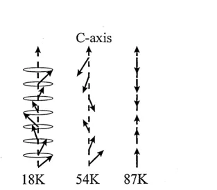
the magnetic structure ofTm were conducted by Koehler et at. (1962) using neutron scattering techniques. These studies reported the paramagnetic to antiferromagnetic

transition occurring at 56 K, at zero field. Similar to Er, the magnetic moments are

sinosoidally modulated along the c-axis. The magnetic moment squares up along the c-..

axis below 40 K and at temperatures below 32 K Tm becomes ferrimagnetic, see figure

, 2.4. In the ferrimagnetic phase the moments are aligned along the c-axis such that the

-sequence of the magnetic moments are 4 layers up and 3 layers down. If an external

field greater than 2.8 T is applied parallel to the c-axis the ferrimagnetic phase is

transformed to a ferromagnetic phase. The total momentum is described by J

=

t

C-axis

•

t

I

• •

~

I

,

~

__ t __ ,

•

\

•

,

t

t :

..

_{-+ -..}

"-l-j

t

_"

t

,

,

t

t

,

t

32K

42K

56K

Figure 2.5. Magnetic ordering ofTm. Ferrimagnetic ordering below 32 K. Square-up

[Coqblin, 1977]. The measured magnetic moment per atom was 7.06J..1.B in the

ferromagnetic state and 1.025 J..I.B in the ferrimagnetic state [Astrom et al. , 1991]. The

magnetic phase diagram of Tm has also been constructed from thermal expansion and

magneto stricti on data [Zochowski and McEwen, 1992] [Willis and Ali, 1991]. Detail of

the magnetic structure in the ferrimagnetic as well as the ferromagnetic phase have been

reported by McEwen et al. (1995), Steigenberger et al. (1992) and McEwen et al ..

(1991) using neutron diffraction. Bohr et al. (1990) reported the use of synchrotron

x-ray diffraction for the study of magnetic ordering in Tm.

There have been no reported ultrasound measurements for Tm and this work is

the first study of the magnetic properties of Tm using ultrasonic techniques.

References

Atoji M. 1974, Solid State Commun., 14, ppl047.

Astrom H.U., Nogues J., Nicolaides G.K., Rao K.V. and Benediktsson G. 1991 1. Phys::

Condens. Matter 3, pp7395-7402.

Bar'yakhtar and Turov 1988, Spin Waves and Magnetic Excitations Vol. 2, Elsevier

Bohr J., Gibbs D.and Huang K. 1990, Physical Review B, 42, no.7, pp4322-4327.

Buchel'nikov V.D and Vasil'ev A.N. 1992, Sov. Phys. Usp., 35, no.3, pp192-21 1.

Coqblin B. 1977, The Electronic Structure of Rare-Earth Metals and Alloys: the

Magnetic Heavy Rare-Earths, Acadamic Press.

Cowley R.A. and Jensen J. 1992, J. Phys. Condens. Matter 4 pp9673-9696.

Eccleston R.S. and S.B. Palmer 1992, J. Magnetism and Magnetic Materials, 104-107,

ppl529-1530.

Edit. by Elliot R.J. 1972, Magnetic Properties of Rare Earth Metals, Plenum Press, chpt

3.

Gibbs D., Bohr J., Axe J.D., Moncton D.E. and D' Arnico K.L. 1986, Phys. Rev. Lett. 55

pp234.

Edit. Gschneider K.A Jr. and Eyring L.R 1978, Handbook On The Physics And

Chemistry Of Rare-Earths, North-Holland.

Habenschuss M., Stavis C., Sinha S.K. Deckman H.W. and Spedding F.H. 1974, Phys.

Hall H.T., Barnett J.D. and Merrill L. 1963, Science, 139, pplll.

Hellier A.G., Palmer S.B. and Whitehead D.G., 1975, J. Phys. E, 8. pp 352 - 354.

Jiles D.C. 1979, PhD Thesis, University of Hull.

Koehler W.C., Cable J.W., Wollan E.O. and Wilkinson, M.K. 1962, Phys. Rev. B 126,

pp1672.

Klemm, B., Z. Anorg. Chem., 1937231 pp150.

McEwen K.A., Steigenberger U. and Jensen J. 1991, Phys. Rev. B, 43, noA,

pp3298-3310.

McEwen K.A., Steigenberger U. Weiss L. Zeiske T. and Jensen J. 1995, J. Magnetism

and Magnetic Materials, pp767-768.

McMarrow D.F., Jehan D.A., Cowley R.A., Eccleston R.S and Mclntyre GJ. 1992, J

Phys.: Condens. Matter, 4, pp8599-8608.

Musgrave MJ.P. 1970, Crystal Acoustics. Intro. To The Study Of Elastic Waves And

Palmer S.B., E.W. Lee and M.N. Islam 1974, Proc. Roy. Soc. Ser. A338, pp341.

Patterson C. 1986, PhD Thesis, University of Hull.

Povey M.J.W., Meredith D.J. and Dobbs E.R. 1980, J Phys. F: Metal Phys., 10

pp2041-53.

Steigenberger U., McEwen K.A., Martinez J.1. and Jensen 1. 1992, Physica B, 181,

ppI58-160.

Snigirev O.V., Tishin A.M. and Volkozub A.V. 1992, J. Magnetism and Magnetic

Materials, 111 ppI49-152.

Truell R., Elbaum C. and Chick B.B. 1969,

Ultrasonic Methods in Solid State Physics,

Academic Press, chpt 1.

Willis F. and Ali N. 1991, J. Appl. Phys. 69, no.8, pp5697-5699 .

. Zochowski S.W. and McEwen K.A 1992" J. Magnetism and Magnetic Materials,

104-107, ppI515-1516.

Zochowski S.W. and McEwen K.A 1992" J. Magnetism and Magnetic Materials,

Chapter 3

Ultrasound Measurement System and Experimental Method

3.0 Introduction

This chapter describes the instrumentation and the experimental procedure used

in the present work where the aim of this work was to set up an automatic ultrasound

measurement system that allows for velocity and attenuation measurements as a

function of (1) temperature, (2) applied magnetic field and (3) ultrasonic frequency.

Before proceeding to describe the system and the modifications made to the original

Matec DSP-8000 software, the shortfall of the original system needs to be addressed

first. To achieve the aim of the work a Matec DSP-8000 ultrasound measurement

system had to be combined with an Oxford Instrument cryogenic and super conducting

magnetic system. The DSP-8000 was not designed to work with the Oxford Instruments

cryogenic and super conducting magnet system. The DSP-8000 software was designed

only to work with a Lakeshore temperature controller and had the limited facility of

controlling only one thermal sensor. As discussed later in this chapter it was found

necessary to introduce an additional thermal sensor to read the sample temperature

. accurately. The original DSP-8000 software had no provision for magnetic field control.

Filters on the AID card were not activated in the original software. Tbe reason for the

filters not to be implemented is because the DSP-8000 system is designed to be used

,. ,

The schematic of the experimental set-up is shown in figure 3.1. The ultrasound

measurement system consisted of; (1) cryostat with super-conducting magnet, (2)

tone-burst generator, (3) digitiser (AID convertor), (4) amplifiers, (5) PC running a modified

version of the Matec DSP-8000 software and (6) transducers.

3.1 The Cryostat And Superconducting Magnet.

The cryostat is a dynamic gas flow type. Figure 3.2 shows a schematic cross

section of the cryostat. The cryostat has an outer protection casing and adjacent to this

is a thin wall vacuum region. In the centre is the Variable Temperature Insert (VTI). The

VTI unit consists of a sample space, heater coils, a temperature sensor and a needle

valve. The needle valve controls the helium flow rate. A servo motor is mounted on top

of the VTI to drive the needle valve. Liquid helium is stored in the lower section of the

cryostat with the superconducting solenoid submerged in the liquid helium. In normal

operation, the low temperature end is at liquid helium temperature of 4.2 K. A lower

temperature of - 1.5 K can be achieved by pumping on the sample space, i.e. increasing

. the helium flow rate and this decreases the vapour pressure above the liquid hence

lowering its temperature._Heating is provided by a 80 W heater coil mounted on a

copper block positioned at the bottom end of the VTI. The sample is placed on a sample

holder which is attached to a sample stick. The sample stick is inseI"!ed into the central

PC RUnning Modified

Servo motor --t~1

Sample

stick --+-+'i"+-~

Sample Holder

Heater coil

and S 1 -of--+-fi~

..-~;:::::;:::::;-- VTI Unit

Protective casing

~-+-- Vacuum space

.

~--+--+- Liquid He

The cryostat is controlled by the Oxford Instrument ITC503 temperature controller. An Oxford Instrument magnet power supply controls and monitors the magnetic field of the superconducting solenoid coils. Two temperature sensors were used; one as the control sensor (S 1) and the other as the sample sensor (S2). SI is used by the temperature controller to maintain the desired temperature. Both sensors were the cemox type with temperature range from 1.5 K to 300 K. The sensitivity of these sensors drops exponentially from the low to high temperature end. Calibration tables for these sensors are stored in the temperature controller itself, hence giving a direct

temperature reading.

The temperature controller controls the accuracy, stability and response time of the cryostat. A feed back loop activates the heater voltage and the needle valve. First it

looks for the difference between the set temperature and the temperature reading

returned by the control temperature sensor, SI. A temperature difference AT = Tcontrot

sensor - Tset is .then obtained. The voltage applied across the heating coils is proportional

to AT. If AT is non zero and negative the heater voltage is increased, otherwise the opposite occurs. A temperature range is defined such that the voltage across the heater ..

coil is proportional to AT. The heater voltage is set to either full or zero, depending on

the sign of

tiT,

temperature range is referred to as the proportional band and can be adjusted to suit the

in increased time to reach the set temperature and can become impractical. To overcome

this, the error voltage is fed into an integrator and the output from the integrator is then

added to the heater voltage. This is repeated until the error is within the set tolerance.

The integrator itself can cause oscillations which can be prevented by making sure that

the time taken for the voltage to swing from fully on to zero in the presence of a fixed

error in the proportional band is twice the response time constant of the cryostat. A third

control parameter determines the rate of change of the temperature. This is referred to

as the derivative action. For all measurements carried out in this work the default factory

settings of the proportional, integral and derivative values were used. Hence in remote

operation, only the desired temperature value is sent to the temperature controller and

the rest of the temperature control operations were left to the temperature controller.

3.2 Tone-Burst Generator (Matec TB-IOOO)

The tone-burst generator used is a 16-bit 100% IBM compatible plug-in card

providing a frequency range of 0.5 MHz to 20 MHz with 200V peak to peak output

voltage. A gated receiver with filters was built on the board. The gain on the gated

receiver can be software controlled from 0 to 70.0 dB. Other computer controlled

features are the tone burst pulse width, tone burst repetition rate, the filter range and the

rectification modes. The triggering was set to internal and triggers on the positive slope.

3.3 Digitiser (SR-9010)

The sampling rate of the digitiser card can be selected via software, between 781

kHz to 100 MHz in the normal mode of operation but this can be as high as 800 MHz

in equivalent time sampling mode. In the normal mode of operation the digitised data

(maximum of 64 Kbytes) were stored directly into the PC's memory through direct

memory accessing (DMA), whereas in the equivalent time sampling mode, e.g. 800

MHz, the waveform had to be captured 8 times. Each time the TTL trigger is delayed by

a set value. The waveform can then be merged, through software, by interleaving the 8

data sets. A 800 MHz sampling rate can thus be achieved from a basic clock rate of only

·100 MHz.

3.4 Amplifiers

The returning signal was amplified by three different amplifiers. The first

amplifier in the return line was the EMAT adaptor box. The EMA T adaptor box had a

broad band amplifier with maximum gain of 50 dB peaked at 10 MHz. To reduce the

noise level, the output from the pre-amplifier was fed into a narrow band tuneable

. receiver amplifier, with..., 50 dB gain in the region of 10 to 15 MHz. The receiver gain

on the tone-burst card was software controlled from 0 to 70 dB. The sensitivity of the

3.5 The Control and Processing Software

The functions of the control software are; (1) sets and checks the experimental

parameters before data acquisition, (2) activate tone-burst and acquire data and (3) .

process and stores data. Communications between the PC and the instruments are via an

IEEE-488 GPIB (General Purpose Interface Bus). All instruments shown in figure 3.1

can be computer controlled apart from the EMAT adaptor box, the tuned receiver

amplifier and the attenuator. Modifications had to be made to the original Matec

DSP-8000 software for it to be useful in this work. The following modifications and changes

were made;

(1) to control Oxford Instruments (Ol) ITC503 temperature controller,

(2) to control 01 superconducting magnet power supply,

(3) to activate the high pass filters on the tone-burst generator card,

(4) to store the captured data

(5) to record and store readings from an additional temperature sensor, S2, mounted on

the sample holder.

The software was written in C++ for Windows and compiled with a Borland

C++ 4.5 compiler. Since the original software was not written in~house, the

documentation on the software was very limited. This made the task of modifying the

software a tedious one. In

an

files) together. The set of codes contained in each of the object files performs a specific

task, e.g. a global variable object file would contain codes defining variables which are

shared by all the object files. In this example the object file performs the function of

defining the global variables. There were forty one main object files and six libraries in

the original DSP-8000 software. This excludes sub-files, i.e. object files linked to the

main object files. The first task in the software modification process is to identify the

function of each of the files linked to the executable target file. The function of some

files were more obvious than others. Next the handling of data between the files had to

be traced, i.e. to map the flow of information between the files. This tedious

investigative work took several weeks and was further complicated by the fact that the

worker on this project did not have any previous experience programming in C++ for

the Microsoft Windows environment.

'" The description on how the software controls work is best described with an

example and a flow chart. Figure 3.3 shows a software flow chart for a typical

ultrasound measurement. On executing the software, the DSP-8000 file functions as the

main Windows file. It reads the set-up file which contains the GPIB addresses for the

instruments. It also reads the calibration table for the digitiser. On top of the main

window is a list of menus. In performing an ultrasound velocity measurement as a

. function of temperature, the Exec menu is activated from the main window. This is

shown as a lighly shaded box within the DSP-8000 box, see figure 3.3. The DSP-8000

file starts by checking the GPIB addresses of the GPIB board and the instruments

~

connected to the computer. It then looks for the type of measurement to be performed

'DS}?8000 ₆

5

4

Figure 3.3. Software flow chart for a typical ultrasound mesurement. The shaded box

which are listed in an object file called "material". This is not shown in figure 3.3. The

relevant information is provided by the user in the appropriated dialogue windows

generated by the material file before Exec is activated. Other information contained in

the material file are the ultrasound path length, the number of cycles in the tone-burst

and the number of averages required per measurement.

Once the type of measurement is known, in this example the temperature

sequence measurement, the temperature control file is called. The temperature control

file contains the experimental variables, i.e. a list of temperature set points at which the

velocity measW'ement is to be made. It also carries information on the experimental

constants. The experimental constants are the tone-burst frequency, tone-burst output

voltage and the magnitude of the applied magnetic field. The temperatW'e set points are

defined by the user in the temperature setup dialog window before Exec is activated.

These data are then sent to the appropriate instruments via the associated object files e.g.

the ma~net control file is called and the magnitude of the desired applied magnetic field

is then passed onto the magnet power supply. The experimental conditions are checked

before Exec call the tone-burst file which in tW'n activates the tone-burst generator and

arms the digitiser. This triggers the digitiser to captW'e 800 I data points each time. The ..

data are then transferred to the PC's memory by direct memory access (DMA). A

location in the PC memory block had ,to be pre-defined for this purpose and has a fixed

size and location. The data sets are captured repeatedly for the desired number of

averages. In order for the time of flight to be determined by the auto-correlation

~

achieved by pre-defining two time gates over two successive pulse echoes. An initial run

is necessary to locate the echoes and for the gates to be set.

The auto-correlation algorithm is not available from the vendor but a brief

technical note from Technology Development Group Inc., Weston, MA. was made

available. With reference to this technical note, the sequence of the tensor post signal

processing is as follows: With two successive pulse-echoes the first pulse echo is

referred to as the reference pulse and the later pulse echo is referred to as the second

pulse. In a single pass through the sample the first pulse echo can be described as:

rl(t) = p(t) * [(d(t)*b(t - to»*d(t)]*i(t - to) (3.1)

where pet), d(t), r(t) and i(t) are functions for transmitted pulse, single-pass dispersion,

back-wall reflection and receiver impUlse response respectively. * denotes the

convolution operator. The second pulse signal would contain all the functions

convoluted in rl(t) plus a front wall reflection function f(t). The second pulse can be

written as:

r2(t)

=

(3.3)

The "Tensor Post Processing" estimates the convoluted function of the dispersion and

reflection functions; X(t)

=

Figure 3.4a. Reference pulse.

square fit. The apex time of the parabola gives the time of flight. Figure 3.4 a and 3.4 b

show the reference pulse and the second pulse respectively from a typical ultrasound

pulse-echo waveform. Figure 3.4 c shows the demodulated output waveform, i.e. X(t).

The time of flight algorithm was tested on samples with known acoustic

velocities, e.g. aluminium. The data were then compared with those obtained manually

using a digital oscilloscope (LeCroy 9410). Prior to the automated ultrasound

measurement the time of flight measurements at room temperature were carried out to

provide absolute velocity measurements which were then used to set the time gates for

the automated ultrasound measurement system. This procedure had to be applied to all

automated ultrasonic measurements involving a tone-burst as it is possible that the

cycles are incorrectly matched. In most cases by

±

of ~t

=

has an absolute error of

±

of Ilv/v "" 0.0005.

3.5.1 Temperature control file

Described in this section are the modifications made to the C++ codes which

control the temperature controller. The original software was designed to control a

Lakeshore temperature controller but an Oxford Instruments (01) temperature controller

The algorithm of the original temperature control file was used. The

modification is fairly straight forward. The Lakeshore commands were replaced with the

01 ITC503 commands where necessary. Additional commands were required to set the

ITC503 to perform automatic control on the heater current and the gas flow in the

cryostat.

3.5.2 Magnet control file

The function of the magnet control file is to manage the data flow between the

software and the magnet power supply. In contains codes controlling the dialogue

windows through which the user pre-defines the magnitude of the desired applied

magnetic field. The algorithm is based on the one used in the temperature control file.

The super-conducting magnet energising and de-energising sequences are written into

the codes. In. order to change the magnetic field, the persistence mode is deactivated by

bringing the supply current to equal the current in the solenoid. Only then can the heater

switch be turned on allowing the circuit between the power supply and super-conducting

coils to be closed. The magnetic field is then changed by either lowering or increasing

the currentin the super-conductor.

The inclusion of the magnet control file to form part of the execution file is not

straight forward. Initialisation routines managed by the "hardware set-up" object file had

1\\

and stored. This also meant that the dialogue windows for the hardware set-up had to be

changed to include an extra input box for the magnet power supply GPIB address to be

defined.

Modifications were made to the material object file such that an option for

magnetic sequence measurements is made available and the dialogue window associated

with this file had to be changed. This was followed by adding codes in the Exec file in

order for it to recognise this additional measurement type.

Changes had to be made to the data storage codes in order for the magnitude of

the applied field to be stored. The data display routines also had to be changed to allow

for the magnetic field data to be displayed. Definitions of new global variables were

added to the global object file.

3.5.3 Wave-form storage

The original software only allows the storage of the time of flight data as a

function of frequency or temperature. The ultrasound wave-form can be displayed on the

graph window with a normalised signal amplitude as a function of time. A hard copy

can be obtained by printing the contents of the graph window but the raw data of the

wave-form could not be stored. A simple routine was attached to the target file for this

purpose. It stores the non-normalised wave data located in the memory buffer of the PC